A Hybrid Forecasting Model for Electricity Demand in Sustainable Power Systems Based on Support Vector Machine

Abstract

Renewable energy sources, such as wind and solar power, are increasingly contributing to electricity systems. Participants in the energy market need to understand the future electricity demand in order to plan their purchasing and selling strategies. To forecast the electricity demand, this study proposes a hybrid forecasting model. The method uses Kalman filtering to eliminate noise from the electricity demand series. After decomposing the electricity demand using an empirical model, a support vector machine optimized by a genetic algorithm is employed for prediction. The performance of the proposed forecasting model was evaluated using actual electricity demand data from the Australian energy market. The simulation results indicate that the proposed model has the best forecasting capability, with a mean absolute percentage error of 0.25%. Accuracy improved by 74% compared to the Support Vector Machine (SVM) electricity demand forecasting model, by 73% when compared to the SVM with empirical mode decomposition, and by 51% when compared to the SVM with Kalman filtering for noise reduction. Additionally, compared to existing forecasting methods, this study’s accuracy surpasses LSTM by 63%, Transformer by 47%, and LSTM-Adaboost by 36%. The simulation of and comparison with existing forecasting methods validate the effectiveness of the proposed hybrid forecasting model, demonstrating its superior predictive capabilities.

1. Introduction

1.1. Background

Energy plays a crucial role in the economic and social development of nations, attracting widespread attention in global political, economic, and military spheres [1]. In recent years, with the continuous development of the world economy and the advancement of modernization, there has been a noticeable imbalance between global energy supply and demand [2]. This imbalance has intensified pressure on resources and the environment, posing significant challenges to the global energy supply landscape [3]. In the pursuit of carbon neutrality, the global energy structure has undergone significant diversification, with a corresponding increase in the share of renewable energy [4]. Renewable energy itself introduces uncertainty, posing significant challenges to energy management. In response to these challenges, various energy management methods have been proposed, such as price-based energy management of grid-connected renewable energy hubs and the economic management of interconnected, flexible renewable energy hubs based on the Unscented Transformation method [5,6,7]. Additionally, traditional distribution grid systems face severe challenges in terms of flexibility, consistent with the ongoing process of electrification. Meanwhile, various energy storage methods, such as hydrogen storage and compressed air storage systems, have seen further development and applications, further altering the dynamics of the energy landscape [8,9]. As the power system becomes more complex, the microgrid technology has changed rapidly. Simultaneously, the rapid development of smart grid systems has involved more microgrid operators, buyers, and sellers, intensifying competition in the electricity market [10,11]. Patrizi, N. et al. established a self-sustaining smart grid system based on labor economics, focusing on prosumers. Through this system, optimal personalized contracts can be developed between microgrid operators and buyers/sellers [12]. The constructed smart grid system is influenced by fluctuations in energy prices, which are fundamentally affected by electricity demand, i.e., the amount of electricity generated and required. Therefore, forecasting electricity demand for sustainable power systems is crucial.

Electricity demand forecasting is a critical task for the electricity system. It not only provides information for electricity suppliers to plan their operations and enables electricity participants to strategize their buying and selling of electricity, but also assists electricity operators in addressing technical and economic issues [13]. Given that electricity must be balanced within the grid, both overestimating and underestimating electricity demand can lead to problems, such as high operational costs. With the increasing share of renewable energy sources, the output of sustainable power systems becomes more uncertain, imposing higher demands on electricity demand forecasting for sustainable power systems. By forecasting electricity demand for sustainable power systems, these issues can be mitigated. Based on the prediction time horizon, electricity demand forecasting is essentially categorized into three main types: short-term electricity demand forecasting, medium-term electricity demand forecasting, and long-term electricity demand forecasting. Among these forecasting frameworks, short-term electricity demand forecasting has garnered the most attention due to the expansion of competitive electricity markets [14], with numerous forecasting models being employed to achieve short-term electricity demand forecasting.

More and more forecasting models are being developed for short-term electricity demand forecasting, according to a thorough literature review. However, the electricity model itself is highly complex, making it generally difficult to design a model for complex power systems, which limits the development of electricity models. Additionally, since classical statistical models are essentially linear, and electricity demand sequences are clearly nonlinear functions of exogenous variables, the performance of classical statistical models in electricity demand forecasting is relatively low.

In the pursuit of enhanced energy demand prediction, numerous studies have sought improvements in traditional models or adopted hybrid approaches. For instance, Xu and Wang [15] introduced a second-order polynomial to augment the Moving Average (MA) model, giving rise to the Polynomial Curve and Moving Average Combination Projection (PCMACP) model. Similarly, Zhu et al. [16] amalgamated the MA model with the seasonal autoregressive integrated moving average (SARIMA) model for power demand forecasting. Hu [17] conducted energy demand forecasting using a residual GM(1,1) model. Homod et al. [18] innovatively presented a hybrid network structure incorporating the Takagi-Sugeno Fuzzy System (TS-FS) for forecasting Heating, Ventilating, and Air-conditioning (HVAC) energy demand. Peng et al. [19] proposed a spatio-temporal forecasting model employing potential flow to estimate urban energy demand. In a distinct approach, Chang et al. [20] employed Functional Principal Components Analysis (FPCA) to project energy consumption trends up to 2035 for Germany, Italy, the U.S., Brazil, China, and India. These endeavors showcase a diverse range of methodologies aimed at refining the accuracy and efficacy of energy demand prediction models within the evolving landscape of power systems.

Soft-computing techniques are increasingly seen as a promising tool for electricity demand forecasting due to their success in solving the non-linear prediction problem, such as the Grey Model [21], the Long Short Term Memory (LSTM) network [22], the Support Vector Machine (SVM) [23], multi-output feedforward neural network [24], Deep Belief Network [25], Artificial Neural Networks (ANN) [14], Recurrent Neural Network (RNN) [26] and so on. Among these soft-computing techniques, the unique aspect of the SVM in comparison to other techniques is its ability to decrease the generalization error using the structural risk minimization [27], which has been used to forecast electricity demand. MayurBarman et al. [28] used the SVM hybridized with grey wolf optimizer (GWO) to forecast electricity demand in three regional special-event days. Maaouane et al. [29] employed neural network modeling to assess and predict energy demand in the transportation sector of developing countries. In a recent study, Chaturvedi et al. [30] conducted a comparative analysis of various time-series models, including SARIMA, Long Short-Term Memory Recurrent Neural Network (LSTM RNN), and Facebook (Fb) Prophet models, aiming to forecast both the total and peak monthly energy demand in India. Diverging from neural network models, the Support Vector Regression (SVR) model is designed to circumvent issues of local minimization and overfitting. Kazemzadeh et al. [31] applied a hybrid data-mining algorithm for long-term forecasting of electricity peak loads and energy demand, employing the Particle Swarm Optimization-Support Vector Regression (PSO-SVR) method. Ağbulut [32] utilized three machine learning algorithms—deep learning (DL), Support Vector Machine (SVM), and Artificial Neural Network (ANN)—to predict transport-based CO2 emissions and energy demand in Turkey. These studies underscore the versatility of advanced modeling techniques within the realm of power systems, demonstrating their applicability for diverse forecasting challenges and their potential to contribute to sustainable energy management.

But the performance of the SVM greatly depends on the choice of some parameters, such as the kernel parameter and regularization parameter [33]. To ensure a high forecasting accuracy of the SVM, the parameters of the SVM should be selected using effective tools, such as cross-validation (CV) [34], genetic algorithms [35] and particle swarm optimization [22]. The first tool selects the parameters of SVM according to the grid search, and the rest of the tools belong to the heuristic algorithm, which performs better than the first tool.

Although more and more tools have been developed to forecast electricity demand, they still face challenges such as addressing the non-stationary electricity demand time series [22] and noise in the electricity demand series introduced by measurement, recording conversion and transmission [24]. The problem of non-stationary time series can be solved by many data decomposition methods. The wavelet transform [36] and empirical mode decomposition (EMD) [37] are most frequently used to decompose the original electricity demand to the high- and low-frequency sub-series.

In the wavelet transform-based forecasting model, the original electricity demand signal is decomposed into different-frequency sub-series using the wavelet decomposition function and predicted separately using forecasting tools, and the individual forecasting results are combined with the final electricity demand forecasting results using the wavelet reconstruction function [38]. But its main weakness is determining how to select the optimal wavelet basis function and its lack of adaptability, which strongly influences the performance of the wavelet transform.

In the EMD-based forecasting framework, the original electricity demand signal is decomposed into several different intrinsic mode functions (IMFs) and residual series, and then the IMFs and residual series are separately predicted using forecasting tools [39]. Compared with the wavelet transform, the EMD has the unique advantages that it does not need the decomposition function and it is a fully data-driven method.

Derived from the data acquisition and monitoring database, load data serve as the foundation for load forecasting and load characteristic analysis, forming the basis for demand-side load adjustments and control. However, due to channel noise, historical load data may exhibit jagged fluctuations, compromising the accuracy of load forecasting results. This can also adversely affect load characteristic analysis, such as the estimation and analysis of air conditioning loads. Additionally, high-quality load data or accurate load forecasting results are crucial foundations for power system planning and operational scheduling. This becomes particularly evident in the context of future smart grids, emphasizing the paramount importance of reliable data for intelligent grid management. Hence, addressing noise-related issues in the load forecasting process is of paramount importance.

Noise reduction methods have been employed to address noise issues in electricity demand, including techniques like the EMD-based noise reduction method and Kalman filtering. The EMD-based approach treats the first IMF or initial IMFs as noise and removes them from the original electricity demand series, thereby enhancing forecasting accuracy [40]. However, eliminating the first IMF or several initial IMFs from the electricity demand series via the EMD-based method may discard valuable information, particularly regarding sharp signals or singularities present in the IMFs.

Kalman filtering is an optimal estimation algorithm used to predict parameters affected by measurement noise. Unlike estimating sub-series from the original signal, it utilizes standard Kalman filtering system functions. Compared to other denoising methods, Kalman filtering can effectively reduce noise, making it widely used in electricity demand forecasting. Research has shown that it can enhance forecasting accuracy [41,42]. Given the superior denoising capabilities of Kalman filtering, this paper, along with the cited references, employs Kalman filtering and EMD for denoising purposes.

1.2. Contributions

While various forecasting models or hybrid forecasting models have been employed in past studies to enhance the accuracy of electricity demand prediction, particularly through the utilization of Support Vector Machine (SVM) and genetic algorithms, there remains a need for more robust solutions to effectively analyze and forecast electricity demand [26,27,28,29,30,31,32,33]. Therefore, this paper proposes a hybrid forecasting model based on the SVM to improve the accuracy of electricity demand prediction. The proposed hybrid forecasting model is compared with existing prediction models, demonstrating higher accuracy compared to the existing ones. The study proposes a new hybrid forecasting method, but there are still some shortcomings. This study did not investigate the quantitative relationship between load demand and energy prices. Future work could attempt to establish this quantitative relationship, which would facilitate energy management and the management of microgrid and smart grid systems. In addition, external factors such as economic indicators and policy changes were not taken into account in the prediction process of this study. In the future, efforts could be made to enhance the accuracy and robustness of the forecasting model by incorporating these external factors to capture additional sources of variability and uncertainty. Additionally, integration with smart grid and distribution network systems could be considered.

This study develops a hybrid forecasting model based on Kalman filtering, EMD, the SVM, and genetic algorithms to further enhance the prediction accuracy of electricity demand. In simple terms, the prediction values, which originally had low fit when based solely on the SVM, are improved after being processed through the hybrid forecasting model proposed in this paper. The detailed steps of the hybrid forecasting model are as follows:

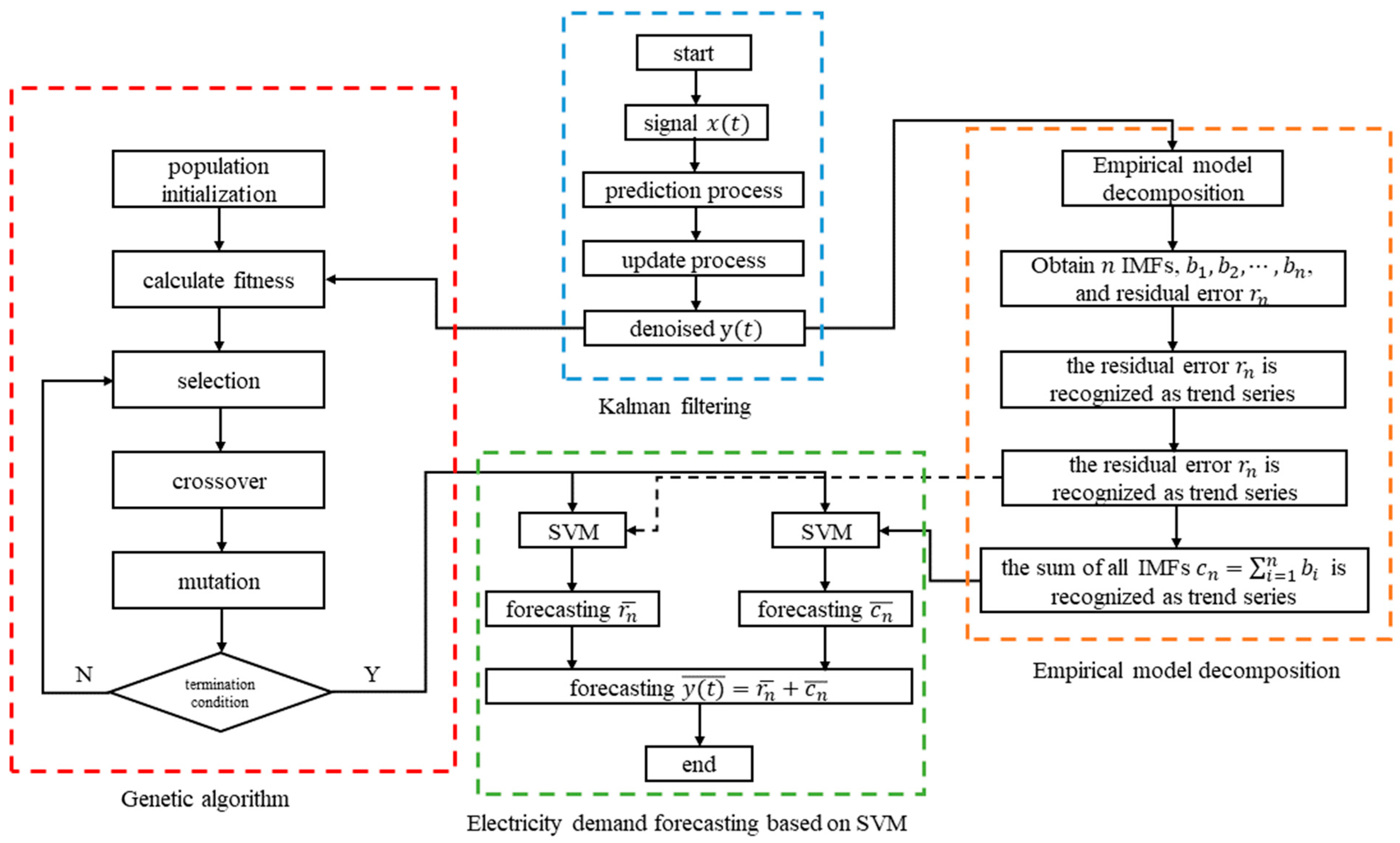
• Utilize Kalman filtering to remove noise signals from the electricity demand series.
• Develop a prediction model using the denoised electricity demand series.
• Utilize EMD to extract sub-trend series, which are residuals from the denoised electricity demand series.
• Finally, model and predict the sub-trend series of the denoised electricity demand series separately using the SVM.

To achieve this objective, the paper first describes the technical approach for creating the hybrid electricity demand forecasting model. Subsequently, a hybrid SVM-based electricity demand forecasting model is established. Finally, the proposed model is evaluated using real electricity demand data from the electricity market.

2. Theoretical Background

2.1. Support Vector Machine

The Support Vector Machine (SVM) is a statistical learning algorithm, which can be used to solve the problems of classification and regression. The SVM has good generalization capabilities. Due to the presence of numerous nonlinear relationships in power load forecasting, traditional statistical methods and regression models often struggle to make accurate predictions. However, the SVM overcomes this by introducing kernel functions, which can map low-dimensional nonlinear problems to high-dimensional spaces, resulting in better data fitting. This capability enables support vector machines to handle complex load variations in power load forecasting, thereby improving prediction accuracy.

Given a training sample set $D=\left\{(x_i,y_i)\right\},1\le i\le N$, the SVM is used to obtain a regression model that makes $f\left(x\right)$ close to $y$ as much as possible, where $f\left(x\right)$ is the regression function represented in Equation (1):

$$f\left(x_i\right)={\omega }^T\phi \left(x_i\right)+b$$

(1)

where $\omega$ is the weight vector, $b$ is the bias, and $\phi \left(x\right)$ is the mapping function that maps the input vector to a higher-dimensional feature space when the sample set is not classified linearly.

Suppose the error between $f\left(x\right)$ and $y$ is $ϵ$, and the loss can be calculated when the absolute error between $f\left(x\right)$ and $y$ is more than $ϵ$. Then, the regression problem can be transformed into Equation (2):

$$\underset{\omega ,b}{\min }{\displaystyle \frac{1}{2}}{\left|\left|\omega \right|\right|}^2+C\sum _{i=1}^N{l}_{ϵ}\left(f\left(x_i\right),y_i\right)$$

(2)

where $l_{ϵ}$ is the $ϵ$-insensitive loss function (see Equation (3)) and $C$ is a predefined positive trade-off parameter between model simplicity and generalization ability. Then, Equation (2) can be rewritten as Equation (4) when the slack variables ${\xi }_i$ and ${\widehat{\xi }}_i$, are introduced to Equation (2).

$$l_{ϵ}\left(Z\right)=\left\{\begin{array}{ll}0,& if \left|z\right|\le ϵ\\ \left|z\right|-ϵ,& otherwise\end{array}\right.$$

(3)

$$\underset{\omega ,b,{\xi }_i,{\widehat{\xi }}_i}{\min }{\displaystyle \frac{1}{2}}{\left|\left|\omega \right|\right|}^2+C\sum _{i=1}^N\left({\xi }_i,{\widehat{\xi }}_i\right)$$

(4)

Subject to:

$$f\left(x_i\right)-y_i\le ϵ+{\xi }_i$$

$$y_i-f\left(x_i\right)\le ϵ+{\widehat{\xi }}_i$$

$${\xi }_i\ge 0,{\widehat{\xi }}_i\ge 0$$

With the most frequently used Gaussian radial function as the mapping function, Equation (5) represents the Gaussian radial function with a width of $g$.

$$K\left(x_i,x_j\right)=\exp \left(-{\displaystyle \frac{{\left|\left|x_i-x_j\right|\right|}^2}{2g^2}}\right),g>0$$

(5)

2.2. Empirical Mode Decomposition

The empirical model decomposition (EMD) is a novel signal processing method that decomposes non-stationary signals into several intrinsic mode functions (IMFs) at different scales, representing fluctuations or trends, in a stepwise manner. It stabilizes the signals, reducing interference or the coupling of characteristic information between them. This paper utilizes EMD to decompose the load sequence into several stationary components at different frequencies. The decomposed components highlight the residual sequence, enabling more accurate load forecasting. The original signals are divided into a number of intrinsic mode functions (IMFs), which are sorted from high-frequency to low-frequency, and a residue, which represents a trend, according to the empirical model decomposition (EMD) proposed by Huang et al. [43]. All IMFs must meet these two requirements: (1) Throughout the whole date series, the difference between extrema and zero-crossings is less than or equal to 1; (2) The mean value of the maxima envelope and the minima envelope formed by local maxima and local minima, respectively, is equal to zero. Given a signal series $x\left(t\right)$, the processes of EMD are summarized as follows:

(1)

Form the maxima and minima envelopes by connecting the local maxima and local minima of original signal $x\left(t\right)$ based on the two cubic spline lines;

(2)

Calculate the mean value series $m\left(t\right)$ of maxima and minima envelopes;

(3)

Determine whether first $\mathrm{c}\mathrm{o}\mathrm{m}\mathrm{p}\mathrm{o}\mathrm{n}\mathrm{e}\mathrm{n}\mathrm{t} h\left(t\right)=x\left(t\right)-m\left(t\right)$ satisfies the two conditions of IMF;

(4)

If it does, $\mathrm{t}\mathrm{h}\mathrm{e} h\left(t\right)$ will be the first IMF and the second IMF will be found using the residue signal $r\left(t\right)=x\left(t\right)-h\left(t\right)$ as a new $x\left(t\right)$;

(5)

If it doesn’t, repeat steps (1) to (2) until the $SD$ is less than 0.2~0.3; then the $h\left(t\right)$ will the first IMF, and step (4) will be repeated to discover the next IM. The screening threshold $SD$ is given as follows:

$${SD}_k=\sum _{t=1}^T{\displaystyle \frac{{\left|h_{i,k-1}\left(t\right)-h_{i,k}\left(t\right)\right|}^2}{h_{i,k-1}^2\left(t\right)}}$$

(6)

Finally, the original signal can be decomposed as follows:

$$x\left(t\right)={\displaystyle \sum _{i=1}^n}IMF\left(I\right)+r\left(n\right)$$

(7)

2.3. Kalman Filter

The proposed hybrid forecasting model harnesses the Kalman filter to predict parameters influenced by measurement noise, such as position, velocity, and direction, while also reducing noise. In situations where variables are only indirectly measurable and measurements from different sensors may be prone to noise, the Kalman filter proves invaluable. Its fundamental principle revolves around estimating the optimal state value at the current moment by considering the current measurement value and the predicted state value derived from the optimal state value at the previous moment. The system functions of the standard Kalman filter are showed in the Equations (8) and (9), where $x_k$ is the state value at the time $k$, $A$ is the state transition matrix, $B$ and $u_k$ is the system parameter, $y_k$ is the measurement value, $C$ is the measurement matrix, and ${\delta }_k$ and ${\epsilon }_k$ are Gauss noise.

$$x_k=A{x}_{k-1}+B{u}_{k-1}+{\delta }_k,{\delta }_k~N\left(0,Q\right)$$

(8)

$$y_k=C{x}_k+{\epsilon }_k,{\epsilon }_k~N\left(0,R\right)$$

(9)

The Kalman filter can be achieved according the prediction process and update process. The prediction process is showed in the Equations (10) and (11), where $P_k$ is the mean square error.

$${\widehat{x}}_k^{-}=A{\widehat{x}}_{k-1}^{-}+B{u}_{k-1}$$

(10)

$$P_k^{-}=A{P}_{k-1}{A}^T+Q$$

(11)

The update process is showed in the Equations (12)–(14), where $K_k$ is the Kalman gain.

$$K_k={\displaystyle \frac{P_k^{-}{C}^T}{C{P}_k^{-}{C}^T+R}}$$

(12)

$${\widehat{x}}_k={\widehat{x}}_k^{-}+K_k\left(y_k-C{\widehat{x}}_k^{-}\right)$$

(13)

$$P_k=\left(I-K_{k}C\right)P_k^{-}$$

(14)

3. Proposed Forecasting Model

This research develops a hybrid forecasting model based on Kalman filtering, EMD, the SVM, and genetic algorithms in order to further increase the forecasting accuracy for electricity demand, and its steps are shown in Figure 1. The accuracy of historical data on electricity demand has a significant impact on the reliability of electricity demand forecasts. Nevertheless, the data gathering process, which includes measurement, recording, conversion, and transmission, introduces noise and uncertainty to the electricity demand series, which poses a serious threat to the model’s ability to predict the future electricity demand accurately. A workable solution to the issue is to utilize the noise reduction method to remove the noise signal from the electrical demand series. In this study, the denoised electricity demand series is utilized to develop the forecasting model after the original electricity demand series has undergone Kalman filtering to remove the noise signal.

Through simulating the trend component rather than just the actual series, the accuracy of the time series model is improved. Hence, the denoised electricity demand series is divided into sub-trend series and non-trend series in this work before being modeled and forecasted, respectively, using the SVM. The EMD may divide a time series into a number of IMFs and residue, with the residue often being known as the time series’ trend component [44]. To extract the sub-trend series from the denoised electricity demand series in this work, the EMD is used. The residual series is then modeled and forecasted based on the SVM. The proposed hybrid forecasting model in this paper first applies Kalman filtering to obtain a denoised electricity demand series. Then, it uses EMD decomposition to extract the required sub-trend series, and models and forecasts these sub-trend series using an SVM optimized by a genetic algorithm.

The machine learning process is highly influenced by the selection of hyperparameters. Currently, various methods are available for hyperparameter selection; for instance, Nurullah Calik et al. [45] use the Tree Parzen Estimator to determine hyperparameters, while You-Gan Wang et al. [46] have proposed an automatic hyperparameter selection method. The performance of Support Vector Machines (SVMs) is significantly affected by the parameters C and g. To enhance the performance of SVMs in electricity demand forecasting, it is crucial to determine the optimal values of C and g. In this paper, a genetic algorithm (GA) is employed to select the optimal values of C and g. The GA parameters are set as follows: a population size of 1000, a crossover probability of 0.85, a mutation probability of 0.05, and a termination condition of achieving accuracy within 10^–5. During training, the Mean Absolute Percentage Error (MAPE) is chosen as the fitness function, and the optimization stops when the fitness function reaches its minimum. The optimization objective of GA is outlined as follows:

$$\underset{C>0,g>0}{\min }MAPE=f\left(C,g\right)$$

(15)

4. Results and Discussion

4.1. Problem Description

This study evaluates the proposed models using real energy market data from Queensland’s electricity market, which were obtained from the Australia Energy Market Operator (AEMO), and covers the period from 1 January 2018 to 31 December 2021. These data are collected every half hour between 00:00 and 24:00, so there are 48 observations every day. This research seeks to forecast the next half hour’s electricity demand using the 70,128 observations from the collected electricity demand series that are displayed in Figure 2.

4.2. Statistics Measures of Forecasting Performance

This paper will use MAPE (Mean Absolute Percentage Error) as the primary criterion to evaluate the forecasting performance. Additionally, Root Mean Square Error (RMSE) and Mean Absolute Error (MAE) will be used as supplementary evaluation criteria. For time series $x_t(t=\mathrm{1,2},\cdots T)$ with the corresponding forecasting time series $\widehat{x_t}$, the MAPE, RMSE and MAE can be calculated as follows.

$$MAPE={\displaystyle \frac{1}{T}}\sum _{t=1}^T\left|{\displaystyle \frac{x_t-\widehat{x_t}}{x_t}}\right|\times 100\%$$

(16)

$$RMSE=\sqrt{{\displaystyle \frac{1}{T}}\sum _{t=1}^T{\left(x_t-\widehat{x_t}\right)}^2}$$

(17)

$$MAE={\displaystyle \frac{1}{T}}\sum _{t=1}^T\left|x_t-\widehat{x_t}\right|$$

(18)

4.3. The Electricity Demand Forecasting

This section presents a comparison of various types of electricity demand forecasting models, including the SVM model, the EMD + SVM (ESVM) model, the Kalman filter + SVM (KSVM) model, and the Kalman filter + EMD + SVM (KESVM) model proposed in this paper. Additionally, analysis and comparisons are performed using the same real-world data for the LSTM model, the improved LSTM model (LSTM-Adaboost), the Transformer model, and the hybrid forecasting model proposed in this paper.

The SVM model is built using the original electricity demand depicted in Figure 2. The characters of electricity demand ($D_t$), the $D_{t-1},$ $D_{t-2},$ $D_{t-3},$ $D_{t-48},$ $D_{t-49},$ $D_{t-50},$ $D_{t-336},$ $D_{t-337},$ $D_{t-338}$ will be the input variables of the SVM model to forecast the $D_t$. Ninety percent and ten percent of the total data will serve as the model’s training and testing datasets, respectively. The normalization method provided in Equation (19) should be used to reduce the magnitude difference between data in all dimensions, which might result in a substantial prediction error, before adding the historical electricity demand data to the SVM model.

$${\overline{D}}_t={\displaystyle \frac{D_t-D_{min}}{D_{max}-D_{min}}}$$

(19)

where the ${\overline{D}}_t$ is the normalized electricity demand series, $D_{min}$ is the minimum electricity demand in the original electricity demand series, and $D_{max}$ is the maximum electricity demand in the original electricity demand series.

The electricity demand series is a non-stationary electricity demand series, which is hardly addressed by the SVM model. Thus, the ESVM model is suggested to deal with this problem. First, the original electricity demand series is broken down by the EMD in the ESVM model into several IMFs ($c_i\left(t\right)$) f, ranging in frequency from the highest- to the lowest-frequency, and a residue error ($e_n\left(t\right)$), which are displayed in Figure 3.

Then, after decomposing the historical electricity demand series into IMFs and the residue error, each $c_i\left(t\right)$ and $e_n\left(t\right)$ will be introduced into the SVM model and then the forecasted $\widehat{c_i}\left(t\right)$ and $\widehat{e_n}\left(t\right)$ will be obtained. Finally, the overall forecasted electricity demand $\widehat{D}\left(t\right)=\sum _{i=1}^{15}\widehat{c_i}\left(t\right)+\widehat{e_n}\left(t\right)$ can be obtained. However, the characteristics of electricity demand will be changed after decomposing the electricity demand series. Thus, the input variables of the ESVM model should be determined again. The partial autocorrelation coefficient (PAC) can guide the selection of input variables for the time series forecasting models, and the lag $k$ PAC of time series $X_t$ is given as Equation (20). Figure 4 shows the partial autocorrelation figure of all IMFs and the residue error.

$${PAC}_{X_t,X_{t-k}|X_{t-1},\cdots ,X_{t-k+1}}={\displaystyle \frac{E\left[\left(X_t-\widehat{E}{X}_t\right)\left(X_{t-k}-\widehat{E}{X}_{t-k}\right)\right]}{E\left[{\left(X_{t-k}-\widehat{E}{X}_{t-k}\right)}^2\right]}}$$

(20)

where $\widehat{E}{X}_t=E\left[X_t|X_{t-1},\cdots ,X_{t-k+1}\right],\widehat{E}{X}_{t-k}=E\left[X_{t-k}|X_{t-1},\cdots ,X_{t-k+1}\right]$.

The input variables of the ESVM model for each IMF and the residue error, as well as the related forecasting outcome, MAPE, are described in

Table 1. The input variables and MAPE of ESVM model.

Sub-Series	Input Variables	MAPE (%)
IMF1	$c_1(t-10)$$,c_1\left(t-9\right),\cdots c_1(t-1)$	156.17
IMF2	$c_2(t-4)$$,c_2\left(t-3\right),\cdots c_2(t-1)$	241.14
IMF3	$c_3(t-4)$$,c_3\left(t-3\right),\cdots c_3(t-1)$	328.84
IMF4	$c_4(t-4)$$,c_4\left(t-3\right),\cdots c_4(t-1)$	66.87
IMF5	$c_5(t-6)$$,c_5\left(t-5\right),\cdots c_5(t-1)$	12.73
IMF6	$c_6(t-5)$$,c_6\left(t-4\right),\cdots c_6(t-1)$	17.85
IMF7	$c_7(t-4)$$,c_7\left(t-3\right),\cdots c_7(t-1)$	11.09
IMF8	$c_8(t-6)$$,c_8\left(t-5\right),\cdots c_8(t-1)$	13.56
IMF9	$c_9(t-4)$$,c_9\left(t-4\right),\cdots c_9(t-1)$	74.98
IMF10	$c_{10}(t-3)$$,c_{10}\left(t-2\right),\cdots c_{10}(t-1)$	7.33
IMF11	$c_{11}(t-1)$	23.06
IMF12	$c_{12}(t-1)$	2.23
IMF13	$c_{13}(t-1)$	1.54
IMF14	$c_{14}(t-1)$	1.87
IMF15	$c_{15}(t-1)$	2.01
Residue error	$c_n(t-1)$	0.16
Sum	/	0.92

based on the results of Figure 4. The MAPE from IMF1 to the residue error shows a declining tendency, as shown in Table 1, and several early IMFs have a comparatively large MAPE due to their high frequency. According to Table 1, the residue error has a minimum MAPE of 0.16%.

The noise signal from the original electrical demand series is removed using the Kalman filtering method. The original electricity demand series and the electricity demand series after noise reduction are shown in Figure 5. Obviously, the denoised electricity demand series ($G$) is smoother than the original electricity demand series.. The parameters of electricity demand remain the same after the noise reduction technique. Hence, the FSVM model uses $G_{t-1},$ $G_{t-2},$ $G_{t-3},$ $G_{t-48},$ $G_{t-49},$ $G_{t-50},$ $G_{t-336},$ $G_{t-337},$ and $G_{t-338}$ as the input variables to forecast the $G_t$.

The accuracy of the forecasting model will be improved to model the trend component in the original series. As shown in Table 1, the MAPE for the residue error, which is always recognized as the trend component, is the minimum. The total of the IMFs is recognized as the non-trend series and the residue error is recognized as the trend series after the denoised electricity demand series is decomposed into numerous IMFs and the residue error. Figure 6 shows the 12 IMFs of the denoised electricity demand. Then, the non-trend series $c_n\left(t\right)=\sum _{i=1}^{12}{b}_i\left(t\right)$ and trend series are obtained and shown in Figure 7. The non-trend series and trend series are introduced into the SVM model to form the KESVM model.

The features of electricity demand vary once the denoised electricity demand is broken down. As a result, the KESVM model’s input variables are verified using the PAC, as illustrated in Figure 8’s partial autocorrelation coefficient figure.

Based on Figure 8, the input variables of the KESVM model for non-trend series and trend series and the corresponding forecasting result, MAPE, are summarized in

Table 2. The input variables and MAPE of KESVM model.

Sub-Series	Input Variables	MAPE (%)
non-trend	$c_n(t-2)$$,c_n\left(t-1\right)$	156.17
trend	$r_n(t-1)$	241.14
sum	/	0.25

.

The forecasting performance of the proposed model are summarized in

Table 3. The MAPE of the electricity demand forecasting models.

Model	SVM	ESVM	FSVM	KESVM
MAPE (%)	0.96	0.92	0.51	0.25
RMSE	121.86	104.59	60.26	30.33
MAE	58.54	54.04	30.41	15.06

.

As shown in Table 3, when the EMD method and the Kalman filter method are combined with the SVM for electricity demand prediction, the forecasting performance based on MAPE can be improved by 4.2% (ESVM) and 46.9% (FSVM), and based on RMSE and MAE, the forecasting performance can be improved by 14.1% and 7.7% (ESVM), and 50.8% and 48.1% (FSVM), respectively. When predicting the non-trend and trend sequences of denoised electricity separately, the forecasting performance based on MAPE can be improved by 74.0% (KESVM), and based on RMSE and MAE, the forecasting performance can be improved by 75.1% and 74.3%, respectively.

Using the same real power demand data, both existing predictive models and the hybrid predictive model proposed in this paper are utilized for prediction, followed by a unified assessment of their predictive accuracy.

As shown in Figure 9, the forecasting results reveal that the proposed hybrid forecasting model exhibits closer proximity to the actual demand curve compared to existing forecasting models. As depicted in Figure 10, the predictive performance of the proposed hybrid forecasting model, based on MAPE, shows a 63% improvement over LSTM, a 47% improvement over Transformer, and a 36% improvement over LSTM-Adaboost. In terms of RMSE-based predictive performance, the proposed hybrid forecasting model outperforms LSTM by 64%, Transformer by 49%, and LSTM-Adaboost by 40%. Regarding the predictive performance based on MAE, the proposed hybrid forecasting model surpasses LSTM by 63%, Transformer by 47%, and LSTM-Adaboost by 38%.

By comparing the proposed hybrid forecasting model with existing forecasting models across various aspects, it becomes evident that the hybrid model proposed in this paper exhibits higher accuracy and better alignment with real data.

5. Conclusions and Future Work

5.1. Conclusions

The accurate prediction of electricity demand is crucial for the economic dispatch of sustainable power systems, guiding not only wind and solar power generation but also the buying and selling strategies of energy market participants. Therefore, this paper proposes a hybrid electricity demand forecasting model that integrates Support Vector Machine (SVM). The model first employs Kalman filtering to eliminate noise from the raw electricity demand series and then applies Empirical Mode Decomposition (EMD) to break down the denoised series. The SVM is then used to model each decomposed series, with optimization performed via a genetic algorithm (GA). Based on simulation results and comparisons with other existing models, the following conclusions can be drawn. The proposed hybrid forecasting model improves accuracy by 74% compared to the SVM electricity demand forecasting model, 73% compared to the SVM with EMD, and 51% compared to the SVM with Kalman filtering. Additionally, compared to existing forecasting methods, the proposed model outperforms LSTM by 63%, Transformer by 47%, and LSTM-Adaboost by 36%. The simulation results and comparisons with existing methods validate the effectiveness of the proposed hybrid forecasting model, demonstrating its exceptional predictive capability. With a forecasting accuracy of up to 99.75%, this model provides a high-precision approach to short-term electricity demand forecasting, offering data support for market participants in formulating their trading strategies.

5.2. Future Work

However, the study still has limitations that warrant further investigation in future research. Specifically, the quantitative relationship between load demand and energy prices was not explored. Future work could focus on establishing this relationship to facilitate energy management and the management of microgrid and smart grid systems. Additionally, external factors such as economic indicators and policy changes were not considered in the prediction process. Incorporating these external factors could enhance the accuracy and robustness of the forecasting model by capturing additional sources of variability and uncertainty. Moreover, integration with smart grid and distribution network systems could be considered as well.

References

1. Dluhopolskyi, O.; Kozlovskyi, S.; Popovskyi, Y.; Lutkovska, S.; Butenko, V.; Popovskyi, T.; Mazur, H.; Kozlovskyi, A. Formation of the model of sustainable economic development of renewable energy. ECONOMICS-Innov. Econ. Res. J. 2023, 11, 51–78. [Google Scholar] [CrossRef]
2. Sahabuddin, M.; Khan, I. Analysis of demand, generation, and emission for long-term sustainable power system planning using LEAP: The case of Bangladesh. J. Renew. Sustain. Energy 2023, 15, 035503. [Google Scholar] [CrossRef]
3. Rao, C.; Zhang, Y.; Wen, J.; Xiao, X.; Goh, M. Energy demand forecasting in China: A support vector regression-compositional data second exponential smoothing model. Energy 2023, 263, 125955. [Google Scholar] [CrossRef]
4. Kazemi, M.; Salehpour, S.Y.; Shahbaazy, F.; Behzadpoor, S.; Pirouzi, S.; Jafarpour, S. Participation of energy storage-based flexible hubs in day-ahead reserve regulation and energy markets based on a coordinated energy management strategy. Int. Trans. Electr. Energy Syst. 2022, 2022, 6481531. [Google Scholar] [CrossRef]
5. Zhang, X.; Yu, X.; Ye, X.; Pirouzi, S. Economic energy managementof networked flexi-renewable energy hubs according to uncertainty modeling by the unscented transformation method. Energy 2023, 278, 128054. [Google Scholar] [CrossRef]
6. Qu, Z.; Xu, C.; Yang, F.; Ling, F.; Pirouzi, S. Market clearing price-based energy management of grid-connected renewable energy hubs including flexible sources according to thermal, hydrogen, and compressed air storage systems. J. Energy Storage 2023, 69, 107981. [Google Scholar] [CrossRef]
7. Pirouzi, S. Transmission and Distribution, Network-constrained unit commitment-based virtual power plant model in the day-ahead market according to energy management strategy. IET Gener. Transm. Distrib. 2023, 17, 4958–4974. [Google Scholar] [CrossRef]
8. Khalafian, F.; Iliaee, N.; Diakina, E.; Parsa, P.; Alhaider, M.M.; Masali, M.H.; Pirouzi, S.; Zhu, M. Capabilities of compressed air energy storage in the economic design of renewable off-grid system to supply electricity and heat costumers and smart charging-based electric vehicles. J. Energy Storage 2024, 78, 109888. [Google Scholar] [CrossRef]
9. Liang, H.; Pirouzi, S. Energy management system based on economic Flexi-reliable operation for the smart distribution network including integrated energy system of hydrogen storage and renewable sources. Energy 2024, 293, 130745. [Google Scholar] [CrossRef]
10. Norouzi, M.; Aghaei, J.; Niknam, T.; Pirouzi, S.; Lehtonen, M. Bi-level fuzzy stochastic-robust model for flexibility valorizing of renewable networked microgrids. Sustain. Energy Grids Netw. 2022, 31, 100684. [Google Scholar] [CrossRef]
11. Norouzi, M.; Aghaei, J.; Pirouzi, S.; Niknam, T.; Fotuhi-Firuzabad, M. Flexibility pricing of integrated unit of electric spring and EVs parking in microgrids. Energy 2022, 239, 122080. [Google Scholar] [CrossRef]
12. Patrizi, N.; LaTouf, S.K.; Tsiropoulou, E.E.; Papavassiliou, S. Prosumer-centric self-sustained smart grid systems. IEEE Syst. J. 2022, 16, 6042–6053. [Google Scholar]
13. Gebremeskel, D.H.; Ahlgren, E.O.; Beyene, G.B. Long-term evolution of energy and electricity demand forecasting: The case of Ethiopia. Energy Strategy Rev. 2021, 36, 100671. [Google Scholar] [CrossRef]
14. Hippert, H.S.; Pedreira, C.E.; Souza, R.C. Neural networks for short-term load forecasting: A review and evaluation. IEEE Trans. Power Syst. 2001, 16, 44–55. [Google Scholar] [CrossRef]
15. Xu, G.; Wang, W. Forecasting China′s natural gas consumption based on a combination model. J. Nat. Gas Chem. 2010, 19, 493–496. [Google Scholar] [CrossRef]
16. Zhu, S.; Wang, J.; Zhao, W.; Wang, J. A seasonal hybrid procedure for electricity demand forecasting in China. Appl. Energy 2011, 88, 3807–3815. [Google Scholar] [CrossRef]
17. Hu, Y.-C. Energy demand forecasting using a novel remnant GM (1, 1) model. Soft Comput. 2020, 24, 13903–13912. [Google Scholar] [CrossRef]
18. Homod, R.Z.; Togun, H.; Abd, H.J.; Sahari, K.S. A novel hybrid modelling structure fabricated by using Takagi-Sugeno fuzzy to forecast HVAC systems energy demand in real-time for Basra city. Sustain. Cities Soc. 2020, 56, 102091. [Google Scholar] [CrossRef]
19. Peng, J.; Kimmig, A.; Niu, Z.; Wang, J.; Liu, X.; Ovtcharova, J. A flexible potential-flow model based high resolution spatiotemporal energy demand forecasting framework. Appl. Energy 2021, 299, 117321. [Google Scholar] [CrossRef]
20. Chang, Y.; Choi, Y.; Kim, C.S.; Miller, J.I.; Park, J.Y. Forecasting regional long-run energy demand: A functional coefficient panel approach. Energy Econ. 2021, 96, 105117. [Google Scholar] [CrossRef]
21. Akay, D.; Atak, M. Grey prediction with rolling mechanism for electricity demand forecasting of Turkey. Energy 2007, 32, 1670–1675. [Google Scholar] [CrossRef]
22. Al-Musaylh, M.S.; Deo, R.C.; Li, Y.; Adamowski, J.F. Two-phase particle swarm optimized-support vector regression hybrid model integrated with improved empirical mode decomposition with adaptive noise for multiple-horizon electricity demand forecasting. Appl. Energy 2018, 217, 422–439. [Google Scholar] [CrossRef]
23. Bedi, J.; Toshniwal, D. Deep learning framework to forecast electricity demand. Appl. Energy 2019, 238, 1312–1326. [Google Scholar] [CrossRef]
24. An, N.; Zhao, W.; Wang, J.; Shang, D.; Zhao, E. Using multi-output feedforward neural network with empirical mode decomposition based signal filtering for electricity demand forecasting. Energy 2013, 49, 279–288. [Google Scholar] [CrossRef]
25. Qiu, X.; Ren, Y.; Suganthan, P.N.; Amaratunga, G.A. Empirical Mode Decomposition based ensemble deep learning for load demand time series forecasting. Appl. Soft Comput. 2017, 54, 246–255. [Google Scholar] [CrossRef]
26. Kong, W.; Dong, Z.Y.; Jia, Y.; Hill, D.J.; Xu, Y.; Zhang, Y. Short-term residential load forecasting based on LSTM recurrent neural network. IEEE Trans. Smart Grid 2017, 10, 841–851. [Google Scholar] [CrossRef]
27. Karthika, S.; Margaret, V.; Balaraman, K. Hybrid short term load forecasting using ARIMA-SVM. In Proceedings of the Innovations in Power and Advanced Computing Technologies (i-PACT), Vellore, India, 21–22 April 2017. [Google Scholar]
28. Barman, M.; Choudhury, N.B. A similarity based hybrid GWO-SVM method of power system load forecasting for regional special event days in anomalous load situations in Assam, India. Sustain. Cities Soc. 2020, 61, 102311. [Google Scholar] [CrossRef]
29. Maaouane, M.; Chennaif, M.; Zouggar, S.; Krajačić, G.; Duić, N.; Zahboune, H.; ElMiad, A.K. Using neural network modelling for estimation and forecasting of transport sector energy demand in developing countries. Energy Convers. Manag. 2022, 258, 115556. [Google Scholar] [CrossRef]
30. Chaturvedi, S.; Rajasekar, E.; Natarajan, S.; McCullen, N. A comparative assessment of SARIMA, LSTM RNN and Fb Prophet models to forecast total and peak monthly energy demand for India. Energy Policy 2022, 168, 113097. [Google Scholar] [CrossRef]
31. Kazemzadeh, M.-R.; Amjadian, A.; Amraee, T. A hybrid data mining driven algorithm for long term electric peak load and energy demand forecasting. Energy 2020, 204, 117948. [Google Scholar] [CrossRef]
32. Ağbulut, Ü. Forecasting of transportation-related energy demand and CO2 emissions in Turkey with different machine learning algorithms. Sustain. Prod. Consum. 2022, 29, 141–157. [Google Scholar] [CrossRef]
33. Liu, Y.; Liao, S. Kernel selection with spectral perturbation stability of kernel matrix. Sci. China Inf. Sci. 2014, 57, 1–10. [Google Scholar] [CrossRef]
34. Liu, Y.; Liao, S. Granularity selection for cross-validation of SVM. Inf. Sci. 2017, 378, 475–483. [Google Scholar] [CrossRef]
35. Wu, C.H.; Tzeng, G.H.; Goo, Y.J.; Fang, W.C. A real-valued genetic algorithm to optimize the parameters of support vector machine for predicting bankruptcy. Expert Syst. Appl. 2007, 32, 397–408. [Google Scholar] [CrossRef]
36. Deo, R.C.; Wen, X.; Qi, F. A wavelet-coupled support vector machine model for forecasting global incident solar radiation using limited meteorological dataset. Appl. Energy 2016, 168, 568–593. [Google Scholar] [CrossRef]
37. Xiong, T.; Bao, Y.; Hu, Z. Interval forecasting of electricity demand: A novel bivariate EMD-based support vector regression modeling framework. Int. J. Electr. Power Energy Syst. 2014, 63, 353–362. [Google Scholar] [CrossRef]
38. Shao, Z.; Chao, F.; Yang, S.L.; Zhou, K.L. A review of the decomposition methodology for extracting and identifying the fluctuation characteristics in electricity demand forecasting. Renew. Sustain. Energy Rev. 2016, 75, 123–136. [Google Scholar] [CrossRef]
39. Huang, N.E.; Shen, Z.; Long, S.R.; Wu, M.C.; Shih, H.H.; Zheng, Q.; Yen, N.C.; Tung, C.C.; Liu, H.H. The empirical mode decomposition and the Hilbert spectrum for nonlinear and non-stationary time series analysis. Proc. R Soc. Lond. Ser. A Math. Phys. Sci. 1971, 454, 903–995. [Google Scholar] [CrossRef]
40. Boudraa, A.O.; Cexus, J.C. EMD-Based Signal Filtering. IEEE Trans. Instrum. Meas. 2007, 56, 2196–2202. [Google Scholar] [CrossRef]
41. Ko, C.N.; Lee, C.M. Short-term load forecasting using SVR (support vector regression)-based radial basis function neural network with dual extended Kalman filter. Energy 2013, 49, 413–422. [Google Scholar] [CrossRef]
42. Takeda, H.; Tamura, Y.; Sato, S. Using the ensemble Kalman filter for electricity load forecasting and analysis. Energy 2016, 104, 184–198. [Google Scholar] [CrossRef]
43. Blood, E.A.; Krogh, B.H.; Ilic, M.D. Electric power system static state estimation through Kalman filtering and load forecasting. In Proceedings of the Power and Energy Society General Meeting—Conversion and Delivery of Electrical Energy in the 21st Century, Pittsburgh, PA, USA, 20–24 July 2008. [Google Scholar]
44. Bedi, J.; Toshniwal, D. Empirical mode decomposition based deep learning for electricity demand forecasting. IEEE Access 2018, 6, 49144–49156. [Google Scholar] [CrossRef]
45. Calik, N.; Güneş, F.; Koziel, S.; Pietrenko-Dabrowska, A.; Belen, M.A.; Mahouti, P. Deep-learning-based precise characterization of microwave transistors using fully-automated regression surrogates. Sci. Rep. 2023, 13, 1445. [Google Scholar] [CrossRef] [PubMed]
46. Wang, Y.G.; Wu, J.; Hu, Z.H.; McLachlan, G.J. A new algorithm for support vector regression with automatic selection of hyperparameters. Pattern Recognit. 2023, 133, 108989. [Google Scholar] [CrossRef]
Figure 1. Schematic of proposed forecasting model.
Energies 17 04377 g001
Figure 2. The electricity demand of Queensland.
Energies 17 04377 g002
Figure 3. IMFs obtained after decomposing electricity demand series.
Energies 17 04377 g003
Figure 4. The partial autocorrelation coefficient figure of IMFs and residue error.
Energies 17 04377 g004
Figure 5. The original electricity demand series and denoised electricity demand series.
Energies 17 04377 g005
Figure 6. The IMFs of denoised electricity demand series.
Energies 17 04377 g006
Figure 7. The non-trend and trend series of the denoised electricity demand series. (a) The non-trend series of the denoised electricity demand series; (b) The trend series of the denoised electricity demand series.
Energies 17 04377 g007
Figure 8. The partial autocorrelation coefficient figure of non-trend and trend series.
Energies 17 04377 g008
Figure 9. Electricity demand of existing prediction models and KESVM.
Energies 17 04377 g009
Figure 10. Predictive accuracy of existing models and KESVM.
Energies 17 04377 g010