A Novel VSG with Adaptive Virtual Inertia and Adaptive Damping Coefficient to Improve Transient Frequency Response of Microgrids

Abstract

This paper proposes a combined adaptive virtual Inertia and adaptive damping control of a virtual synchronous generator (AID-VSG) to improve the dynamic frequency response of microgrids. In the proposed control scheme, the VSG’s virtual inertia and damping coefficients adapt themselves during the transients to, respectively, reduce frequency deviations and increase the oscillations’ damping. In addition, as an important feature, the proposed AID-VSG is suitable for distributed control scheme applications and is designed to not rely on phase-locked loop (PLL) measurements, which avoids PLL stability issues on weak grids. The control parameters of the proposed AID-VSG are tuned by the particle swarm optimization (PSO) algorithm to minimize the overshoot and settling time of the microgrid’s frequency during an islanding event. The AID-VSG is validated by a comparative analysis with three existing VSG control schemes, also tuned by the stated optimization algorithm. The performance of each compared VSG strategy is evaluated through the simulation of a set of 10,000 initial conditions, using the islanded microgrid’s nonlinear model. The best response among the VSG strategies was achieved by the proposed AID-VSG control for both the optimization problem and the set of initial conditions’ simulations.

1. Introduction

Microgrids are composed of clusters of loads, distributed generators (DGs), and energy storage systems (ESSs) that may be operated as single controllable entities [1]. In the case of grid-connected microgrids, they are connected to a large power network at the point of common coupling (PCC) and their capability of operating in islanded mode increases the resiliency and reliability of distribution systems [2].

Typically, most DGs and ESSs are connected to the power network through power electronic interfaces [3]. However, unlike synchronous generators (SG), power electronic converters do not possess intrinsic inertia and damping characteristics.

Thus, when a microgrid operates with increasing penetration of energy resources interfaced by power converters, its equivalent inertia becomes smaller, jeopardizing the microgrid’s dynamic frequency response [4,5]. The issue of lack of inertia can be challenging even for large power systems, as highlighted in the ENTSO-E position paper [6], which lists the lack of inertia as one of the main challenges for future power systems with large shares of renewable energy sources. The UK 2019 blackout analysis also revealed that the reduction in inertia was one of the factors contributing to the power outage [7].

Several control schemes have been proposed within the virtual synchronous generator (VSG) concept to overcome the lack of inertia of power converters [8]. The VSG, with its ability to emulate the dynamic characteristics of a conventional SG by introducing virtual inertia and damping properties [9,10], offers a supporting level of adaptability to the power converter. Hence, compared to the SG, the VSG is very flexible as its virtual inertia and damping coefficient can be adjusted to improve frequency performance and stability [11,12].

To further improve the contribution of power converters’ control on microgrid dynamic frequency response, researchers have been proposing alterations to the conventional VSG control by inserting additional loops [13,14,15,16,17] or developing self-adaptive loops to act on the VSG’s virtual inertia [18,19,20,21,22,23,24,25,26,27], the VSG’s damping coefficient [28], or both VSG’s virtual inertia and damping [29,30,31,32,33].

To highlight the research gap covered in this paper, the above-mentioned papers are classified in

Table 1. Research gap definition.

Reference	Considers Adaptive Inertia	Considers Adaptive or Additional Damping	Dispenses Frequency Measurements	Considers Constant Droop Gain at Steady-State	Considers Off-Nominal Frequency	Includes Fixed-Inertia Machine
[21]	✓	✗	✓	✓	✓	✗
[18,25]	✓	✗	✓	✓	✗	✓
[20,23,26,27]	✓	✗	✓	✓	✗	✗
[22]	✓	✗	✗	✓	✓	✗
[19,24]	✓	✗	✗	✓	✗	✓
[13]	✗	✓	✗	✓	✗	✓
[14,15,17]	✗	✓	✓	✓	✓	✗
[16,28]	✗	✓	✓	✗	✗	✗
[32]	✓	✓	✗	✓	✓	✓
[33]	✓	✓	✓	✗	✗	✗
[30,31]	✓	✓	✓	✗	✓	✗
[29]	✓	✓	✓	✓ 1	✗	✗
Proposed paper	✓	✓	✓	✓	✓	✓

¹ Constant droop gain in [29] is achieved through a rule-based controller, which may cause a continuous switching behavior in the damping coefficient when operating in off-nominal frequency.

according to their contributions to particular issues within microgrid’s frequency control studies. Concerning the issues addressed in Table 1, the following observations are drawn:

• Adapting both the VSG’s virtual inertia and damping coefficient may contribute positively to microgrids’ transient response, and only a few papers employ both adaptations in the VSG control;
• Despite the adaptations, maintaining a constant steady-state frequency droop is a required feature to preserve the VSG’s contribution in the primary frequency control;
• Relying on the grid’s frequency measurements, a phase-locked loop (PLL), for example, is an undesired feature, as the PLL itself may lead to instabilities [2];
• The control’s performance must be evaluated under off-nominal steady-state frequency operation (e.g., for islanded microgrid operation) once the adaptive strategies operate using the VSG’s frequency signal, and most of them were originally designed for operation around nominal frequency;
• The presence of SGs in microgrids is desirable for frequency regulation. These machines have fixed inertia and damping properties, so the VSG’s inertia must be carefully tuned to avoid, for example, undamped oscillatory responses in the SGs.

As presented in Table 1, all the abovementioned issues are addressed in this paper, whose main contributions are summarized as follows:

• The proposal of a new VSG control strategy with adaptive virtual inertia and adaptive damping coefficient (AID-VSG). The proposed AID-VSG differs from existing adaptive inertia and damping strategies as it maintains the desired steady-state frequency droop (unlike [30,31,33]) and does not rely on frequency measurements (unlike [32]) or rule-based controllers (unlike [29]);
• The validation of the proposed AID-VSG by comparison with three existing VSG control strategies (optimally tuned for off-nominal frequency operation), for a large set of initial conditions.

The remaining part of the paper is organized as follows: Section 2 presents three VSG control strategies from the literature, and the proposed AID-VSG is presented in Section 3. To illustrate the potential of the compared VSG control strategies in the transient frequency response, Section 4 presents a case study in which the islanding of a microgrid is simulated with different parameter settings for each VSG control. For a fair comparison, the VSG control strategies are automatically tuned by an optimal tuning proposed and discussed in Section 5. The optimally tuned VSGs are then validated by simulations of a large set of initial conditions in Section 6. Finally, Section 7 concludes the article.

2. VSG Control Strategies for Power Converters

In this section, three of the existing VSG control schemes proposed in the literature are introduced, and a brief discussion of the effects of their adjustable parameters on the transient frequency response is drawn. These strategies provide a theoretical basis on which the proposed adaptive VSG control will be developed, and they will be used for comparison with the AID-VSG control.

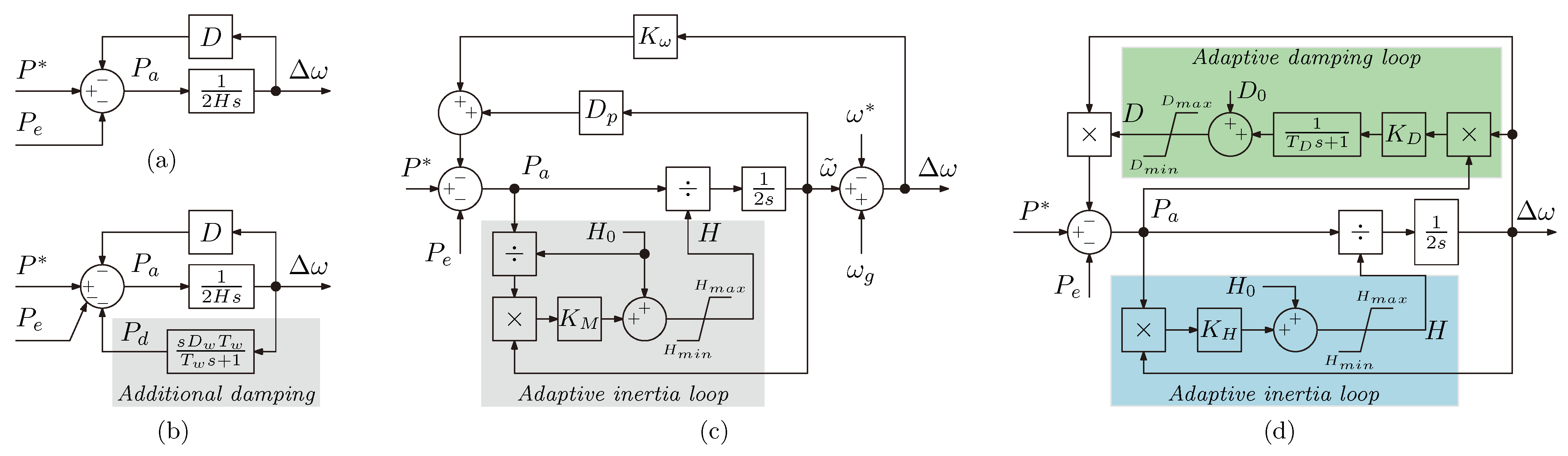
2.1. VSG with Fixed Parameters

The conventional VSG frequency regulation-based active power loop (APL) with fixed inertia and damping coefficient (hereinafter referred to as “FP-VSG”) is shown in Figure 1a. The APL emulates the rotor motion equation of a synchronous generator as follows [20]:

$$\Delta \dot{\omega }\left(t\right)={\displaystyle \frac{P_a\left(t\right)}{2H}}={\displaystyle \frac{P^{*}-P_e\left(t\right)-D\Delta \omega \left(t\right)}{2H}},$$

(1)

where H is the virtual inertia, and D is the virtual damping coefficient of the VSG. The frequency deviation $\Delta \omega$ is defined by the difference between the VSG virtual frequency ${\omega }_{VSG}$ and the nominal (or reference) frequency ${\omega }^{*}$ (i.e., $\Delta \omega ={\omega }_{VSG}-{\omega }^{*}$), $P^{*}$ is the VSG’s reference input power, and $P_e$ is the electrical measured power at the VSG’s output. The virtual power angle $\delta$ is obtained through the integration of the $\Delta \omega$ signal in rad/s, i.e., $\dot{\delta }\left(t\right)={\omega }_s\Delta \omega \left(t\right)$, with ${\omega }_s$ the synchronous angular frequency.

If the fast dynamics of inner voltage and current control loops are not considered [34], the voltage-controlled VSG can be represented by a voltage source behind a virtual impedance $Z_V$ [35]. If the voltage regulation loops are not considered in the VSG, the magnitude of the voltage source is kept constant.

As $\Delta \omega \left(t\right)$ is defined as a deviation from the reference frequency, PLLs are not needed in the FP-VSG as the grid’s frequency measurement is not required. This also implies that D acts both as the damping coefficient during the transients and as the droop gain within the primary frequency control, at a steady state.

Although both H and D are parameters that can be set at the VSG to obtain a desired transient frequency response, adjusting D to modify the transients may be unwanted as it changes the VSG’s contribution in the primary frequency control.

2.2. VSG with Fixed Parameters and Additional Damping Loop

From the conventional APL in Figure 1a, it can be seen that the transient frequency response may be improved by an additional loop feeding the frequency oscillations back to the accelerating power through a washout filter, as adopted in [14] (hereafter, referred to as “AD-VSG”) and shown in Figure 1b and (2) and (3).

$${\dot{P}}_D\left(t\right)=-{\displaystyle \frac{P_D\left(t\right)}{T_w}}+D_w{\displaystyle \frac{P_a\left(t\right)}{2H}}$$

(2)

with $P_a$ defined as follows:

$$P_a\left(t\right)=P^{*}-P_e\left(t\right)-P_D\left(t\right)-D\Delta \omega \left(t\right).$$

(3)

In this case, both H and D are constant and the transient response can be adjusted by the additional damping power $P_D$, according to the transient gain $D_w$ and the washout filter time constant $T_w$. Due to the cascaded washout filter, $D_w$ only affects the transient response. Thus, the steady-state frequency droop remains unchanged, given by D.

2.3. VSG with Adaptive Virtual Inertia

Reference [24] presents an adaptive inertia VSG strategy (referred to as “AI-VSG”) by substituting the VSG’s fixed virtual inertia with a time-varying virtual inertia $H\left(t\right)$, according to its frequency deviation and angular acceleration, which is defined as follows:

$$H\left(t\right)=\left\{\begin{array}{cc}{h}_a\left(t\right)\hfill & \mathrm{if}{H}_{min}<h_a\left(t\right)<H_{max}\hfill \\ H_{min}\hfill & \mathrm{if}{h}_a\left(t\right)\le H_{min}\hfill \\ H_{max}\hfill & \mathrm{if}{h}_a\left(t\right)\ge H_{max}\hfill \end{array}\right.$$

(4)

where

$$h_a\left(t\right)=H_0+K_M{\displaystyle \frac{P_a\left(t\right)}{H_0}}\tilde{\omega }\left(t\right),$$

(5)

$$P_a\left(t\right)=P^{*}-P_e\left(t\right)-D_p\tilde{\omega }\left(t\right)-K_{\omega }\Delta \omega \left(t\right),$$

(6)

and illustrated in Figure 1c. The parameters $H_0$ and $K_M$ represent the nominal value for virtual inertia and the adaptive inertia gain, respectively. Also, upper ($H_{max}$) and lower ($H_{min}$) bounds are used to limit the adaptive virtual inertia H value. Depending on whether the frequency is deviating from its steady-state value or returning to it, the inertia is increased or decreased, respectively [24].

In [24], the VSG’s frequency deviation $\tilde{\omega }$ used in the adaptive inertia law is defined as the difference between the VSG’s frequency and the grid’s frequency ${\omega }_g$ ($\tilde{\omega }\triangleq {\omega }_{VSG}-{\omega }_g$). In this case, the virtual damping coefficient $D_p$ does not act as a droop, because at a steady state ($\tilde{\omega }=0$), it has no contribution to the control signal. Thus, the primary frequency control is solely provided by the droop gain $K_{\omega }$.

As can be seen, to implement the adaptive virtual inertia proposed in [24], the grid frequency needs to be measured by a PLL or some other frequency estimation strategy (in this work, a first-order model with a time constant of 20 ms was used to approximate the PLL dynamics [36] in the grid frequency measurement).

For fixed values of $H_0$ and $K_{\omega }$ or D, the benefits of implementing the adaptive virtual inertia AI-VSG in the transient frequency response may be evaluated by altering the adaptive inertia gain $K_M$. As the adaptive inertia influences solely the inertial loop, this adaptive control does not change the steady-state power–frequency behavior.

3. Proposed Adaptive Virtual Inertia and Adaptive Damping VSG Control

This section presents the proposed transient adaptive virtual inertia and damping coefficient VSG control strategy (AID-VSG). The proposed technique consists of substituting the constant virtual inertia and damping coefficient with time-varying signals, as presented below.

The adaptive virtual inertia is inspired by the one presented in [24]; however, two alterations are made. The first alteration directly replaces $K_M/H_0$ in (5) with a new adaptive inertia gain $K_H$, which does not impose changes in the adaptive virtual inertia adaptation from [24] since both $K_M$ and $H_0$ are constant values freely set in the AI-VSG. The second alteration eliminates the need for PLLs or other grid frequency measurements in the adaptive VSG control by replacing $\tilde{\omega }$ in (5) and (6) with $\Delta \omega$, such that (6) becomes the following:

$$P_a\left(t\right)=P^{*}-P_e\left(t\right)-(D_p+K_{\omega })\Delta \omega \left(t\right),$$

(7)

which generates an equivalent equation for $P_a$ as the one presented in (1) for the conventional VSG, with $D=D_p+K_{\omega }$. Since now the equivalent virtual damping coefficient $D=D_p+K_{\omega }$ in (7) is multiplied by $\Delta \omega$, it also acts as the droop gain at a steady state, which in turn constrains its design to meet the primary frequency control requirements.

Comparing (7) and (6), one may see that the VSG control loses transient damping by removing the frequency grid measurement from the AI-VSG since the term $D_p\tilde{\omega }$, which only acts during the transients, is no longer available. To compensate for this loss of transient damping caused by removing the PLL, the constant virtual damping coefficient D is then replaced by a time-varying signal $D\left(t\right)$, such that the proposed AID-VSG control implements the virtual swing equation as follows:

$$\Delta \dot{\omega }\left(t\right)={\displaystyle \frac{P_a\left(t\right)}{2H\left(t\right)}}={\displaystyle \frac{P^{*}-P_e\left(t\right)-D\left(t\right)\Delta \omega \left(t\right)}{2H\left(t\right)}},$$

(8)

in which the adaptive virtual inertia is given by the following:

$$H\left(t\right)=\left\{\begin{array}{cc}{h}_a\left(t\right)\hfill & \mathrm{if}{H}_{min}<h_a\left(t\right)<H_{max}\hfill \\ H_{min}\hfill & \mathrm{if}{h}_a\left(t\right)\le H_{min}\hfill \\ H_{max}\hfill & \mathrm{if}{h}_a\left(t\right)\ge H_{max}\hfill \end{array}\right.$$

(9)

with

$$h_a\left(t\right)=H_0+K_H{P}_a\left(t\right)\Delta \omega \left(t\right),$$

(10)

and the adaptive virtual damping coefficient $D\left(t\right)$ is as follows:

$$D\left(t\right)=\left\{\begin{array}{cc}{d}_t\left(t\right)\hfill & \mathrm{if}{D}_{min}<d_t\left(t\right)<D_{max}\hfill \\ D_{min}\hfill & \mathrm{if}{d}_t\left(t\right)\le D_{min}\hfill \\ D_{max}\hfill & \mathrm{if}{d}_t\left(t\right)\ge D_{max}\hfill \end{array}\right.$$

(11)

with

$$d_t\left(t\right)=D_0+d_a\left(t\right),$$

(12)

$${\dot{d}}_a\left(t\right)=-{\displaystyle \frac{d_a\left(t\right)}{T_D}}+{\displaystyle \frac{K_D}{T_D}}{P}_a\left(t\right)\Delta \omega \left(t\right).$$

(13)

In practice, the time-varying virtual coefficient $D\left(t\right)$ is given by the sum of a reference virtual damping coefficient $D_0$ and an adaptive signal composed of the low-pass filtered product of $P_a\left(t\right)$ and $\Delta \omega \left(t\right)$, i.e., the same signal used for the virtual inertia adaptation, bounded by upper ($D_{max}$) and lower ($D_{min}$) limits. $K_D$ is the adaptive damping gain, and $T_D$ is the time constant of the first-order filter, and both are tunable parameters within the adaptive control. The block diagram for the proposed AID-VSG is presented in Figure 1d.

The first-order low-pass filter is included in the adaptive damping loop to allow the combined adaptive virtual inertia and damping controls to act in different time frames during transients: the virtual inertia loop will act just after the occurrence of the disturbance to prevent a significant frequency decline, while the loop of virtual damping will provide additional transient damping to the frequency oscillations after the initial inertial response.

Steady-State Performance

At the equilibrium point, both $\Delta {\dot{\omega }}^{ss}=0$ and ${\dot{d}}_a^{ss}=0$ (the superscript $ss$ denotes steady-state values). As $H^{ss}$ will always be a positive real value due to the minimum and maximum bounds in $H\left(t\right)$, from (8), we obtain the following:

$$0={\displaystyle \frac{P_a^{ss}}{2H^{ss}}}\Rightarrow P_a^{ss}=0,$$

(14)

therefore, (10) becomes

$$h_a^{ss}=H_0+K_H{P}_a^{ss}\Delta {\omega }^{ss}\Rightarrow h_a^{ss}=H_0,$$

(15)

and (13) becomes

$$0=-{\displaystyle \frac{d_a^{ss}}{T_D}}+{\displaystyle \frac{K_D}{T_D}}{P}_a^{ss}\Delta {\omega }^{ss}\Rightarrow d_a^{ss}=0,$$

(16)

which leads to the following:

$$d_t^{ss}=D_0+d_a^{ss}\Rightarrow d_t^{ss}=D_0.$$

(17)

Thus, from (9) and (11), it is derived that the adaptive virtual inertia and the adaptive virtual damping at a steady state in the proposed AID-VSG are given by $H_0$ and $D_0$, respectively.

In the proposed AID-VSG, $D_0$ may be designed to couple with the steady-state requirements, i.e., the adaptive virtual damping coefficient loop does not change the primary frequency control contribution of the VSG, given by $D_0$.

Small-Signal Stability Assessment

This section presents the results of a small-signal stability assessment for the nonlinear model of a multi-machine system with the proposed AID-VSG control. This analysis verifies the convergence of the AID-VSG’s adaptive inertia and damping coefficient to their reference values when the multi-machine system is operated in its equilibrium point’s vicinity.

Let us consider a multi-machine with $n_g$ SGs represented by the classical model and with $n_v$ AID-VSGs. Assuming that the n-th machine’s power angle (with $n=n_g+n_v$) is the angular reference [37], the dynamic behavior of the system is represented by the 2$n-1+n_v$ nonlinear system as follows:

$${\dot{\delta }}_{in}\left(t\right)={\dot{\delta }}_i\left(t\right)-{\dot{\delta }}_n\left(t\right)={\omega }_s\left(\Delta {\omega }_i\left(t\right)-\Delta {\omega }_n\left(t\right)\right),1\le i\le n-1$$

(18)

$$\Delta {\dot{\omega }}_i\left(t\right)=\left\{\begin{array}{cc}{\displaystyle \frac{1}{2}}{\displaystyle \frac{{P^{*}}_i-{P_e}_i\left(t\right)-({D_0}_i+{d_a}_i\left(t\right))\Delta {\omega }_i\left(t\right)}{{H_0}_i+{K_H}_i\left({P^{*}}_i-{P_e}_i\left(t\right)-\left({D_0}_i+{d_a}_i\left(t\right)\right)\Delta {\omega }_i\left(t\right)\right)\Delta {\omega }_i\left(t\right)}}\hfill & ,1\le i\le n_v\hfill \\ {\displaystyle \frac{1}{2}}{\displaystyle \frac{{P_m}_i-{P_e}_i\left(t\right)-D_i\Delta {\omega }_i\left(t\right)}{H_i}}\hfill & ,n_v+1\le i\le n\hfill \end{array}\right.$$

(19)

$$\dot{{d_a}_i}\left(t\right)=-{\displaystyle \frac{{d_a}_i\left(t\right)}{{T_D}_i}}+{\displaystyle \frac{{K_D}_i}{{T_D}_i}}\left({P^{*}}_i-{P_e}_i\left(t\right)-({D_0}_i+{d_a}_i\left(t\right))\Delta {\omega }_i\left(t\right)\right)\Delta {\omega }_i\left(t\right),1\le i\le n_v$$

(20)

In (19), ${P_m}_i$, $H_i$ and $D_i$ are the mechanical power, the inertia, and the damping coefficient of the i-th SG. The remaining variables and parameters in (18)–(20) have already been defined, and the subscript i relates them to the i-th machine (either an SG or a VSG).

Linearizing (18)–(20) around the equilibrium point ${\delta }_{ij}={\delta }_{ij}^e$, $\Delta {\omega }_i=0$, and ${d_a}_i=0$, the multi-machine linearized system is given by the following:

$$\Delta {\dot{x}}_a=A_a\Delta x_a,$$

(21)

with

$$\Delta x_a={\left[\begin{array}{ccccccccc}\Delta {\delta }_{1n}& \cdots & \Delta {\delta }_{(n-1)n}& \Delta {\omega }_1& \cdots & \Delta {\omega }_n& {d_a}_1& \cdots & {d_a}_{n_v}\end{array}\right]}^T,$$

(22)

and $A_a$ is the linearized state matrix. Since both ${H_0}_i$ and ${D_0}_i$ are predefined parameters, for simplicity of representation we use ${H_0}_i=H_i$ and ${D_0}_i=D_i$. Thus, the linearized state matrix can be written as follows:

$$A_a=\left[\begin{array}{cccccccccc}0& \cdots & 0& {\omega }_s& \cdots & 0& -{\omega }_s& 0& \cdots & 0\\ ⋮& \ddots & ⋮& ⋮& \ddots & ⋮& ⋮& ⋮& \ddots & ⋮\\ 0& \cdots & 0& 0& \cdots & {\omega }_s& -{\omega }_s& 0& \cdots & 0\\ J_{11}& \cdots & J_{1(n-1)}& \frac{-D_1}{2H_1}& \cdots & 0& 0& 0& \cdots & 0\\ ⋮& \ddots & ⋮& ⋮& \ddots & ⋮& ⋮& ⋮& \ddots & ⋮\\ J_{(n-1)1}& \cdots & J_{(n-1)(n-1)}& 0& \cdots & \frac{-D_{(n-1)}}{2H_{(n-1)}}& 0& 0& \cdots & 0\\ J_{n1}& \cdots & J_{n(n-1)}& 0& \cdots & 0& \frac{-D_n}{2H_n}& 0& \cdots & 0\\ 0& \cdots & 0& 0& \cdots & 0& 0& \frac{-1}{T_{D_1}}& \cdots & 0\\ ⋮& \ddots & ⋮& ⋮& \ddots & ⋮& ⋮& ⋮& \ddots & ⋮\\ 0& \cdots & 0& 0& \cdots & 0& 0& 0& \cdots & \frac{-1}{T_{D_{nv}}}\end{array}\right]$$

(23)

with

$$J_{pq}=-{\displaystyle \frac{1}{2H_p}}{E}_p^{\prime }{E}_q^{\prime }\left|Y_{pq}\right|sin\left({\delta }_{pq}^e-{\theta }_{pq}\right),$$

(24)

for $p\ne q$. When $p=q$, $J_{pq}=J_{pp}$ is computed as follows:

$$J_{pp}={\displaystyle \frac{1}{2H_p}}\sum _{\begin{array}{c}j=1\\ j\ne p\end{array}}^n{E}_p^{\prime }{E}_j^{\prime }\left|Y_{pj}\right|sin\left({\delta }_{pj}^e-{\theta }_{pj}\right)$$

(25)

where $E_i^{\prime }$ is the machine’s internal voltage, and $|Y_{ij}|$ and ${\theta }_{ij}$ are the absolute value and phase angle of the appropriate element in the transfer admittance matrix [37].

The state matrix $A_a$ in (23) can be represented in a more compact way as follows:

$$A_a=\left[\begin{array}{cc}{A}_c& 0_{2n-1,n_v}\\ 0_{n_v,2n-1}& T\end{array}\right],$$

(26)

where $A_c$, with dimension $(2n-1)\times (2n-1)$, is the multi-machine linearized system for a power system with n machines (e.g., $n_g$ SGs and $n_v$ VSGs) represented by the classical model [37]; $0_{i,j}$ is a zero matrix with i rows and j columns; and T is the diagonal matrix in which the i-th diagonal element is given by $-1/{T_D}_i$.

For stability assessment, the eigenvalues of $A_a$ are computed by solving for $\lambda$ using the following:

$$det(\lambda I-A_a)=0.$$

(27)

Applying the Laplace expansion to compute $det(\lambda I-A_a)$, we can obtain

$$\begin{array}{c}\hfill det(\lambda I-A_a)=\prod _{k=1}^{n_v}\left(\lambda +{\displaystyle \frac{1}{{T_D}_k}}\right)det(\lambda I-A_c)=0\end{array}$$

(28)

From (28), we may conclude that the linearized system for the multi-machine power system with AID-VSGs has $2n-1$ eigenvalues, which are the same as those of $A_c$ for the system with conventional VSGs, and also $n_v$ eigenvalues associated with the adaptive damping coefficient time constant ${T_D}_k$, i.e.,:

$${\lambda }_k={\displaystyle \frac{-1}{{T_D}_k}},k=1,\dots ,n_v.$$

(29)

Since ${T_D}_k$ is a positive constant, if small-signal stability is guaranteed for the multi-machine system with conventional VSG control (FP-VSG with $H_i$ and $D_i$), it is also guaranteed for the linearized system of the multi-machine power system with AID-VSGs (with ${H_0}_i=H_i$ and ${D_0}_i=D_i$).

4. Case Study

This section presents a case study to evaluate the performance of the presented VSG control strategies, under different parameter tuning conditions, on the transient frequency response of a microgrid during an islanding occurrence.

4.1. Microgrid’s Description

Let us consider a medium-voltage (MV) microgrid, as presented in Figure 2, composed of 13 buses, 2 diesel-based synchronous generators, and 1 battery energy storage system (BESS). The microgrid is connected to the main grid at the PCC by switch SW1. The upstream grid is represented by an equivalent high-voltage network with a 5000 MVA short circuit power and 10 X/R ratio. The loads are presented as constant impedances, and the lines in the model are shown as short lines, obtained from the equivalent balanced three-phase system presented in [38], and power transformer data are given in

Table 2. Power transformer data.

Transf.	Voltage	Rated Power	Impedance 1
TR1	115/12.47 kV	12 MVA	0.08 + j9.97%
TR2	12.47/0.48 kV	6 MVA	3.334 + 5.773%

¹ Percentage impedance refers to a common base power of 10 MVA.

. The total load power is 7.32 MVA with a 0.9 power factor.

Each SG (G1 and G2, in Figure 2) has a rated power of 3 MVA and is represented by a sixth-order model [37]. Voltage regulation at both diesel generators is modeled by ST2C AVR with power factor controller type 2 obtained from [39]. The speed regulation is generated by a primary frequency control as in [40]. The SG’s inertia constant is 0.3 s, and other model parameters are presented in Appendix A.

The BESS connected to bus 10 has 6 MVA of rated power. The VSG control is applied to the BESS with no voltage regulation, acting as an ideal voltage source behind a reactive virtual impedance of 25.5%. Steady-state active power is regulated by the steady-state virtual damping coefficient, adopted as $D=10$ p.u. in this work.

In the grid-connected operation mode, each energy resource is assumed to be providing 1.5 MW of active power and no reactive power to the grid. Thus, the microgrid has a deficit in the active power of approximately 2.8 MW, which must be shared among diesel and BESS for the islanded operation mode.

To assess the transient performance of each VSG control strategy and its effects on the microgrid’s frequency response when an islanding procedure occurs, an unintentional microgrid’s transition from the grid-connected mode to islanded mode was simulated, considering different values for the VSG control strategies’ parameters.

The time-domain simulations were conducted in ANATEM—version 11.10.2 (ANATEM is a software used by Brazilian TSO to perform nonlinear analysis of electromechanical transients developed by the Brazilian Electric Energy Research Center (CEPEL)), from which some performance indices, namely the settling time $t_s$ (the settling time is defined by the time required for an output signal to reach and steady within a set tolerance band, specified as $2\%$ in this work), and the minimum value of frequency (or frequency nadir, $f_{nad}$) were obtained in the MATLAB R2018b environment. The simulation results are presented in the next section.

4.2. Microgrid’s Islanding Simulations with the Existing VSG Techniques

Concerning the FP-VSG control, Figure 3 presents the transient frequency response at the PCC (bus 1 in Figure 2) and also in the VSG and the SG (since both SGs have the same control and parameters, the same transient frequency response is observed on both. Thus, one single curve represents the frequency response of both SGs) for the microgrid islanding simulation considering different values of FP-VSG virtual inertia, ranging from $H=0.3$ s to $H=30$ s. When the FP-VSG’s inertia is set to 0.3 s (defined in this work as the reference case, as the virtual inertia is the same as the SGs’ inertia), a more significant deviation is observed in the three displayed transient frequencies due to the low equivalent inertia, implicating a frequency nadir of 59.20 Hz at the microgrid’s PCC. As presented in Figure 3, the frequency nadir is improved by increasing the FP-VSG’s virtual inertia. However, larger values for H introduce an oscillatory behavior in the microgrid’s frequency due to the oscillations of the small-inertia SGs against the large-inertia VSG’s frequency and may even slow the transient frequency response, increasing the settling time ($t_s$), as displayed in

Table 3. Performance indices for the existing VSG techniques.

FP-VSG			AD-VSG			AI-VSG
$\mathit{H}$	${\mathit{f}}_{\mathit{nad}}$	${\mathit{t}}_{\mathit{s}}$	${\mathit{D}}_{\mathit{w}}$	${\mathit{f}}_{\mathit{nad}}$	${\mathit{t}}_{\mathit{s}}$	${\mathit{K}}_{\mathit{M}}$	${\mathit{f}}_{\mathit{nad}}$	${\mathit{t}}_{\mathit{s}}$
0.3 s	59.20 Hz	2.97 s	5 p.u.	59.36 Hz	3.00 s	$5·{10}^3$ p.u.	59.30 Hz	2.97 s
1.5 s	59.43 Hz	3.04 s	10 p.u.	59.48 Hz	3.01 s	$25·{10}^3$ p.u.	59.40 Hz	2.96 s
14 s	59.56 Hz	2.42 s	20 p.u.	59.55 Hz	2.93 s	$10·{10}^4$ p.u.	59.47 Hz	2.94 s
30 s	59.56 Hz	6.75 s	50 p.u.	59.56 Hz	4.72 s	$10·{10}^6$ p.u.	59.49 Hz	2.97 s

.

To evaluate the benefits of including the additional transient damping loop in the AD-VSG, Figure 4 presents the transient frequency response for the microgrid’s islanding for different values of the transient gain $D_w$. The AD-VSG’s virtual inertia and damping coefficient are the same as the reference case, i.e., $H=0.3$ s and $D=10$ p.u., respectively. The time constant was adopted as the same from [14], i.e., $T_w=0.5$ s. As presented in Figure 4 and Table 3, the frequency nadir is improved with the increase in $D_w$. Compared to the FP-VSG, the AD-VSG causes a less oscillatory response in the transient frequency of the PCC and the SG, as shown in Figure 4a,c. However, due to its fixed inertia, increasing $D_w$ in the AD-VSG has little effect in reducing the VSG frequency slope, i.e., the rate of change in frequency (RoCoF), just after the islanding occurrence, as can be seen by comparing Figure 4b to Figure 3b. The frequency slope is roughly the same for $D_w$ between 5 and 20 p.u, and it is slightly better for $D_w=50$ p.u.; nevertheless, this higher transient gain increases the settling time (Table 3), slowing the transient response.

For the VSG with time-varying virtual inertia (AI-VSG), simulations were conducted with $H_0=0.3$ s (which is the same value as the reference case); $D_p=50$ p.u., as adopted in [24]; $K_{\omega }=10$ p.u. to meet the desired primary control; and $H_{min}=0.01$ s and $H_{max}=14$ s, so as to avoid a close to zero virtual inertia or excessively slow settling time, respectively. The results obtained from the microgrid islanding simulation for different values of $K_M$ are presented in Figure 5 and the performance indices from the transient frequency at the PCC are listed in Table 3. Similar to the previous cases, the frequency nadir is improved by the increase in $K_M$. However, the changes in $K_M$ mainly alter the frequency transient response before $t=1.5$ s, causing the settling time to be roughly the same (around 2.95 s as shown in Table 3). This can be explained by the fact that the adaptive inertia with grid frequency measurement mainly acts when there is a significant difference between the frequency of the VSG and the frequency of the grid. Thus, after both the grid and the VSG frequencies start to settle, the frequency oscillation is primarily given by the one obtained with the fixed inertia control (note that the settling time for the FP-VSG with $H=0.3$ s, in Table 3, is 2.97 s, i.e., close to those obtained by the AI-VSG control). This behavior is due to the fact that the AI-VSG focuses on transient stability, i.e., on preventing generators from losing step one from another, and on limiting the RoCoF and nadir.

4.2.1. Limitations of the Existing VSG Techniques on Altering Transient Frequency Response

The results presented for the existing VSG techniques have shown that the microgrid’s transient frequency response can be improved either through a new tuning of the conventional VSG control (FP-VSG) or through the addition of transient loops (AD-VSG and AI-VSG). However, some limitations still exist in the application of the existing techniques, as summarized in the following observations:

• To provide additional inertial support by reducing the frequency slope, the FP-VSG demands higher values of virtual inertia, which introduces a more oscillatory and possibly slower response;
• The AD-VSG allows for an improvement in the frequency nadir; however, the additional loop is less effective in reducing the frequency slope without increasing the settling time, as this loop was designed to increase damping, and no adaptive inertia was added;
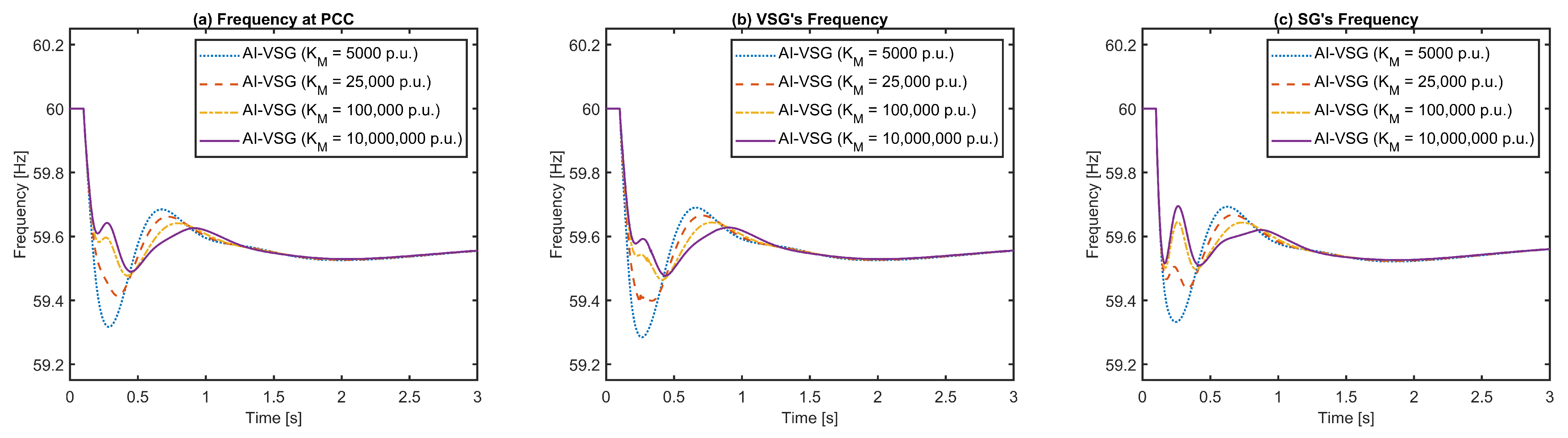
• The AI-VSG provides transient additional inertial support but slightly changes the transient response time, since one of AI-VSG’s main goals was to improve transient stability instead of acting on the settling time.

4.3. Microgrid’s Islanding Simulations with the Proposed AID-VSG

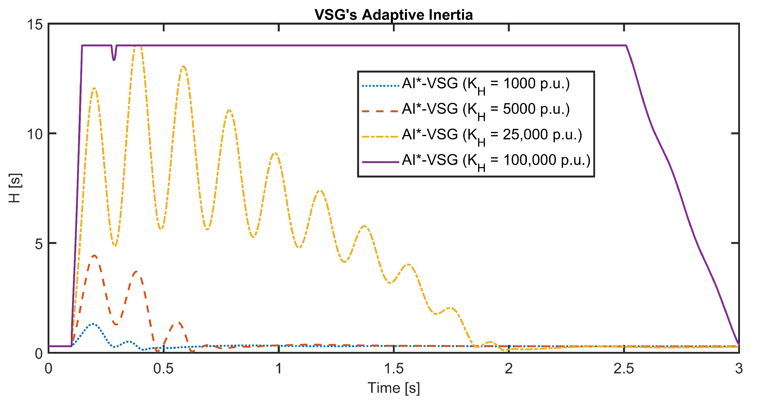
To evaluate the effectiveness of the proposed AID-VSG in overcoming the abovementioned limitations and to illustrate the effects of its parameters tuning in the microgrid’s frequency transient response, three analyses are conducted in this section. For all three of them, the nominal virtual inertia is kept at $H_0=0.3$ s; the nominal damping coefficient is set as $D_0=10$ p.u. (to match the desired primary frequency control); and the lower and upper bounds of adaptive inertia are set as $H_{min}=0.01$ s and $H_{max}=14$ s, respectively. To avoid a null value in the virtual damping coefficient, its lower bound is set as $D_{min}=0.01$ p.u., while $D_{max}=50$ p.u. is set to avoid excessively high values. $T_D$ is set to 0.5 s, as $T_w$ from [14] in the AD-VSG. The adaptive gains $K_H$ and $K_D$ are altered among the analyses.

4.3.1. AI*-VSG

The first analysis aims to evaluate exclusively the removal of the grid’s frequency measurement (PLL) in the adaptive inertia loop, which is performed by forcing $K_D=0$ in the proposed AID-VSG. For simplicity, this case is referred to as AI*-VSG, as only the inertia adapts itself during the transients. The results for the microgrid islanding simulation with $K_D=0$ and different values of $K_H$ are presented in Figure 6. One can observe that improvements in frequency nadir are obtained by increasing $K_H$. However, as $K_H$ increases, the transient frequency response of the microgrid becomes similar to that obtained by FP-VSG control with $H=14$ s, which is due to the increasing values in the adaptive virtual inertia, as presented in Figure 7, and explained below. For example, with $K_H=100,000$, the VSG’s frequency in Figure 6b changes slowly and with no significant oscillations. Since the VSG’s frequency deviation from its reference value ($\Delta \omega$) is mainly decreasing, $P_a$ and $\Delta \omega$ are both negative and will cause the virtual inertia to increase. Due to the high adaptive gain $K_H$, the virtual inertia will be increased until saturation, and the VSG will behave as a high-inertia machine, causing the SG’s frequency to oscillate around the VSG’s frequency during the time interval in which the virtual inertia is saturated.

Comparing the results for the AI*-VSG case (Figure 6) to the AI-VSG control (Figure 5), it can be noticed that removing the frequency measurements in the VSG’s adaptive inertia control deteriorates the oscillations’ damping, mainly for higher adaptive inertia gains. However, it also allows for more effective action in decreasing the VSG’s frequency slope at the transient’s beginning, as seen in Figure 6b.

Concerning the time response of the AI*-VSG, from the settling times in

Table 4. Performance indices for the proposed AID-VSG control.

AI*-VSG (${\mathit{K}}_{\mathit{D}}=0$)			AID-VSG (${\mathit{K}}_{\mathit{H}}=3·{10}^3$ p.u.)			AID-VSG (${\mathit{K}}_{\mathit{D}}=5·{10}^5$ p.u.)
${\mathit{K}}_{\mathit{H}}$	${\mathit{f}}_{\mathit{nad}}$	${\mathit{t}}_{\mathit{s}}$	${\mathit{K}}_{\mathit{D}}$	${\mathit{f}}_{\mathit{nad}}$	${\mathit{t}}_{\mathit{s}}$	${\mathit{K}}_{\mathit{H}}$	${\mathit{f}}_{\mathit{nad}}$	${\mathit{t}}_{\mathit{s}}$
$1·{10}^3$ p.u.	59.36 Hz	2.95 s	0 p.u.	59.48 Hz	2.92 s	0 p.u.	59.53 Hz	3.00 s
$5·{10}^3$ p.u.	59.53 Hz	2.89 s	$1·{10}^5$ p.u.	59.54 Hz	2.88 s	$3·{10}^3$ p.u.	59.56 Hz	2.11 s
$25·{10}^3$ p.u.	59.52 Hz	2.69 s	$3·{10}^5$ p.u	59.55 Hz	2.72 s	$5·{10}^3$ p.u.	59.56 Hz	2.25 s
$10·{10}^4$ p.u.	59.55 Hz	4.16 s	$5·{10}^5$ p.u	59.56 Hz	2.11 s	$75·{10}^2$ p.u.	59.56 Hz	2.40 s

, it can be seen that depending on the $K_H$ value, the transient response may become even slower.

4.3.2. AID-VSG with Fixed $K_H$

The second analysis evaluates the effects of introducing the adaptive damping loop by keeping a constant $K_H$ while altering $K_D$. For this, $K_H$ is arbitrarily set as 3000, while $K_D$ varies between 0 and 500,000. The respective results are presented in Figure 8. As the action of the adaptive damping loop is intentionally delayed, we can see in the zoomed-in views that varying the adaptive gain $K_D$ does not change the initial transient response from $t=0.1$ s to around $t=0.2$ s, since the curves are primarily overlapped in this time frame. After the adaptive damping effectively starts to act, we may see that increasing $K_D$ not only improves the frequency nadir but also reduces the amplitude of the frequency oscillations. Concerning the settling time, in Table 4, we observe that varying $K_D$ also makes the transient frequency response faster.

Figure 9 presents the VSG’s adaptive inertia and adaptive damping coefficient for the same values of $K_H$ and $K_D$ in Figure 8 during the islanding simulation. It can be observed from Figure 9a that the most significant changes in inertia occur within the first few hundred milliseconds after the islanding event. In contrast, the damping coefficient adaptation lasts longer, as presented in Figure 9b. Also, it is noted that increasing the adaptive gain $K_D$ reduces the maximum value of the adaptive inertia $H\left(t\right)$. This is because the adaptive damping coefficient $D\left(t\right)$ increases faster when a high $K_D$ is adopted, which in turn starts to reduce the accelerating power used to create the adaptive inertia signal. It is noteworthy that for the different nonzero values of $K_D$, the adaptive inertia starts to return to its reference value (i.e., when it decreases from its peak value) when the adaptive damping coefficient is still rising, which corroborates with the design objective of acting faster in the frequency transient by the inertia adaptation.

4.3.3. AID-VSG with Fixed $K_D$

In the third analysis, $K_D$ is kept constant while $K_H$ varies. Arbitrarily setting $K_D$ = 500,000, Figure 10 presents the transient frequency response results when $K_H$ is varied. When $K_H$ increases, the nadir of frequency is improved, and the frequency deviations are reduced since the first swing. From the zoomed-in view in Figure 10b, it can be seen that since the VSG’s frequency tangent slope is reduced, it becomes clear that increasing $K_H$ results in increasing the VSG’s virtual inertia, which is verified by the adaptive inertia transient response in Figure 11a. It is worth mentioning that the VSG’s frequency tangent slope reduction through increasing the adaptive inertia causes the virtual power angle $\delta$ to change slower than the SG’s power angle, increasing the transient exchange of power between the VSG and the SG, which also increases the VSG’s accelerating power. Thus, by increasing the adaptive inertia gain $K_H$, the accelerating power is also increased in the first swing, and the adaptive damping increases even without changing the adaptive gain $K_D$, as can be seen in Figure 11b. Concerning the settling time $t_s$ presented in Table 4, we notice that increasing the adaptive inertia gain $K_H$ for the same $K_D$ may slow the frequency transient response.

4.3.4. Effects of Both Adaptive Loops on the Frequency at the Microgrid’s PCC

Comparing the zoomed-in views in Figure 8a and Figure 10a, it can be seen that the increase in $K_H$ improves the first local minimum of frequency, while the increase in $K_D$ solely starts to significantly affect the transient response of frequency after 0.2 s. The effects of adaptive inertia and damping loops are consistent with those from conventional fixed inertia and damping coefficient in synchronous generators-based power systems, in which the inertial response acts faster than the dampening response.

Therefore, the AID-VSG control allows for flexibility when controlling the transient frequency response by tuning $K_H$ and $K_D$ according to the needs in limiting frequency slope (RoCoF) or increasing frequency oscillations’ dampening. Furthermore, a faster response may be achieved through a coordinated tuning of both adaptive gains. Thus, the proposed control is well suited to overcome the limitations presented by the existing VSG techniques in Section 4.2.1.

5. Optimal Tuning of the VSG’s Parameters

The simulation results presented in Section 4 provide insights into how each VSG control strategy, by changing its parameters, may affect the transient frequency response of a microgrid during the islanding procedure.

Aiming for a fair comparison among all the presented VSG control strategies, this section proposes the VSG’s parameters tuning for each VSG control strategy through an optimization problem. To this end, we define a mono-objective function given by the weighted sum of two distinct objectives, namely the settling time and the maximum deviation to the steady-state frequency, given as follows:

$$\begin{array}{cccc}\hfill & \underset{\xi }{\min }\hfill & \hfill & w_1{t}_s+w_2\left|f_{nad}-f_{RP}\right|\hfill \\ \hfill & \mathrm{s}.\mathrm{t}.\hfill & \hfill & {\xi }_{min}\le \xi \le {\xi }_{max}\hfill \end{array}$$

(30)

where $w_1$ and $w_2$ are the weights of each objective function, $t_s$ is the settling time, $f_{nad}$ is the minimum value of frequency at the PCC during the transient caused by the microgrid’s islanding, and $f_{RP}$ is the microgrid’s steady-state frequency in the islanded operation mode. Furthermore, $\xi$ represents the set of control parameters to be tuned in each VSG control strategy, which is given as $\xi =\left\{H\right\}$ for the FP-VSG, $\xi =\left\{D_w;T_w\right\}$ for the AD-VSG, $\xi =\left\{K_M\right\}$ for the AI-VSG, and $\xi =\left\{K_H;K_D;T_D\right\}$ for the AID-VSG. In addition, the particular case of the AID-VSG with $K_D=0$, referred to as AI*-VSG, is also tuned, being $\xi =\left\{K_H\right\}$. The control parameters to be tuned are constrained by their minimum and maximum bounds, ${\xi }_{min}$ and ${\xi }_{max}$, respectively.

The optimization problem was solved by the use of the particle swarm optimization (PSO) algorithm, which has often been used to solve optimal tuning of VSGs in microgrids [41,42,43]. To avoid overshoots in the frequency response, the objective function weights were set as $w_1=1$ and $w_2=100$. This implies that even a slight overshoot in frequency (around 0.01 Hz) when multiplied by $w_2$ results in an objective function value of the same magnitude as the settling time. The PSO algorithm parameters are listed in

Table 5. PSO algorithm parameters.

PSO Parameter	Setting
Individual learning rate	1.49
Global learning rate	1.49
Inertia weight	Adaptive from 0.1 to 1.1
Number of particles	100
Number of maximum iterations	100

.

Simulation Results

Table 6. Performance indices after VSG’s optimal tuning.

VSG Strategy	Set of Tuned Parameters $\mathit{\xi }$	${\mathit{f}}_{\mathit{nad}}$	${\mathit{t}}_{\mathit{s}}$
VSG-REF	-	59.20 Hz	2.97 s
FP-VSG	$\left\{13.61\right\}$	59.55 Hz	2.36 s
AD-VSG	$\left\{14.84;0.73\right\}$	59.55 Hz	1.76 s
AI-VSG	$\left\{9.45·{10}^9\right\}$	59.49 Hz	2.93 s
AI*-VSG	$\left\{4.95·{10}^8\right\}$	59.55 Hz	2.42 s
AID-VSG	$\left\{665.72;2.85·{10}^5;0.87\right\}$	59.55 Hz	1.71 s

presents the optimally tuned parameters and the performance indices of the transient frequency response at the microgrid’s PCC after the optimal tuning for each VSG control strategy and also for a reference case (VSG-REF) when fixed inertia is assumed to be the same as the synchronous generators inertia, i.e., $H=0.3$ s.

As can be seen, all the VSG control strategies were able to improve the frequency nadir, increasing it from 59.20 Hz in the reference case to 59.55 Hz, except for the AI-VSG in which the frequency nadir was increased to 59.49 Hz. The fastest response was obtained by the proposed AID-VSG control strategy ($t_s=1.71$ s), closely followed by the AD-VSG control.

Figure 12 displays the comparison of transient frequency for the microgrid’s PCC, the VSG, and the SG for the optimal tuning and the reference case.

Frequency response curves for FP-VSG and AI*-VSG practically overlap, indicating that the high value of adaptive gain $K_H$ causes the adaptive inertia to saturate at the upper bound ($H=14$ s) as the frequency deviates from its nominal value. The small difference between the settling time for these two strategies is because the optimal, tuned inertia for the FP-VSG ($H=13.61$ s) is slightly lower than the upper bound in the adaptive inertia, which makes the FP-VSG slightly faster. However, it is important to note that if the frequency were to return to its nominal value, the AI*-VSG would respond faster than the FP-VSG. Since the grid frequency measurement was used in the AI-VSG, and the AD-VSG and AID-VSG strategies provided additional damping, a less oscillatory frequency response could be observed for these three control strategies when compared to the FP-VSG and AI*-VSG control loops.

Figure 13a presents the VSG’s adaptive inertia for optimal tuning in the AI-VSG, AI*-VSG and AID-VSG control strategies. To achieve the desired performance formulated in the optimization problem, both AI-VSG and AI*-VSG were tuned with large values of adaptive inertia gain, causing the virtual inertia to saturate during the transient. For the AI-VSG, despite the saturation in some intervals within the first seconds, the virtual inertia returned to its nominal value around $t=4$ s, while for the AI-VSG the virtual inertia stayed at its maximum value for most of the transient response. On the other hand, the AID-VSG’s inertia adapted itself without reaching saturation, and it quickly returned to its nominal value.

Figure 13b presents the AID-VSG’s adaptive inertia (blue curve) and damping coefficient (orange curve) in terms of the percentage rate of change in their nominal values, i.e., $H\left(t\right)/H_0$ and $D\left(t\right)/D_0$, respectively. The adaptive parameters’ peak values stayed around 220%, representing a peak value of 0.67 s for the inertia and 22.1 p.u. for the damping coefficient. As previously discussed in Section 4.3, both the adaptive inertia and the damping coefficient contributed in different time frames within the frequency control: the former acted at the transient’s very beginning and its rapid response lasted a few hundred milliseconds, while the latter gradually took over the former, and it lasted a few seconds.

6. Performance Assessment

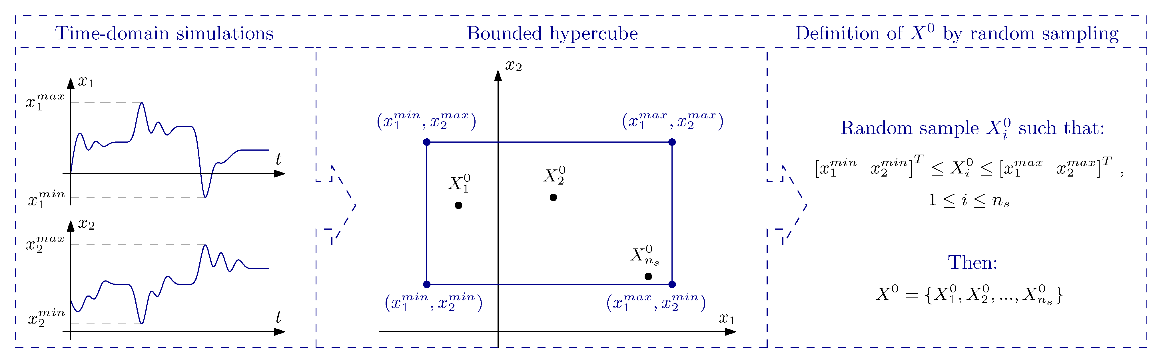
To further evaluate the contributions of each VSG control strategy on the microgrid’s dynamic frequency response during the islanding operation, in this section, we simulate the nonlinear state-space system that models the microgrid for the islanded operation considering a set of different initial conditions $X^0$ for the state variables.

Definition of $X^0$

In this paper, we define the set $X^0$ by a random sampling of $n_s$ initial conditions within the hypercube defined by maximum and minimum values of each state variable, which are obtained through the simulation of a set of disturbances applied to the microgrid in both the grid-connected and islanded mode. This process is conceptually illustrated in Figure 14 for a bi-dimensional state-space system.

The disturbances applied to the microgrid are as follows:

• A three-phase short circuit with a duration of 150 ms at the high voltage side of TR1, followed by the opening of SW1 (i.e., microgrid islanding);
• A step of $25\%$ on the microgrid’s load;
• A step of +1.5 MW on the VSG’s reference power ($P^{*}$);
• A step of $-3.0$ MW on the VSG’s reference power ($P^{*}$);
• A step of +1.5 MW on the VSG’s reference power ($P^{*}$).

After the time-domain simulation of the mentioned disturbances and the definition of the hypercube by the minimum and maximum values of the state variables, the set $X^0$ was defined by the random sampling of initial conditions considering $n_s$ = 10,000.

The set $X^0$ was then used as initial conditions for the time-domain simulations of the islanded microgrid for each one of the VSG control strategies tuned in Section 5 and also for the reference case, which is the VSG control with $H=0.3$ s.

As severe disturbances (such as the three-phase short-circuit) were included to generate the range of initial conditions, instead of evaluating the frequency at the PCC, we assessed the frequency of each generator to verify if its transient response could cause their protection schemes to trip.

Therefore, in each one of the $n_s$ time-domain simulations conducted for each considered VSG control strategy, the maximum and minimum values of frequency for both the SG and the VSG were stored, and a graphical statistical analysis of these data is presented through the box plot graphs shown in Figure 15. Reference lines are inserted into the graphs to represent the nominal frequency and instantaneous tripping settings within the under-frequency (function 81U) and over-frequency (function 81O) protection scheme.

Concerning the VSG maximum frequency deviations, i.e., graphs presented in Figure 15a,c, it is possible to conclude that the VSG strategies that provide the best performances were FP-VSG, AI*-VSG, and AID-VSG, as they presented a narrower range in frequency deviations. On the other hand, regarding the SG maximum frequency values, as shown in Figure 15b, better results were obtained with the VSG-REF, AD-VSG, AI*-VSG, and AID-VSG control strategies, while for the SG minimum frequency values, as shown in Figure 15d, the VSG-REF, AD-VSG, AI-VSG, and AID-VSG control strategies performed better. Thus, by applying the proposed AID-VSG control, a narrower range in frequency deviations can be obtained for both the VSG and the SG.

In Figure 15, violations of the under/over frequency limits for all VSG control strategies are observed, caused by some of the simulated initial conditions. To better show the prevalence of these violations in each control strategy,

Table 7. Percentile of transgressions of under or over frequency limits.

VSG Strategy	Percentile of Occurrences
VSG-REF	0.84%
FP-VSG	25.47%
AD-VSG	0.57%
AI-VSG	1.85%
AI*-VSG	10.18%
AID-VSG	0.51%

shows the percentile of these initial conditions that cause violations of the maximum frequency deviations in one or both generator frequencies (SG or VSG).

Even though the control strategies FP-VSG and AI*-VSG present reduced ranges of maximum deviation in the VSG’s frequency (Figure 15), from Table 7, higher numbers of frequency transgression occurrences can be observed for these VSG control strategies, since high virtual inertia in the VSG ends up causing the synchronous generator’s frequency to oscillate around the VSG’s frequency.

Compared to the FP-VSG and the AI*-VSG, the VSG-REF presents a smaller number of frequency transgressions; however, transgressions on both the VSG and the SG frequencies (Figure 15) can be observed in this VSG control strategy, as both generators present low inertia.

When comparing the VSG control strategies with adaptive inertia with and without the grid frequency measurement (AI-VSG and AI*-VSG, respectively), even though the range of frequency variation is larger in the AI-VSG, its percentile of frequency transgressions is smaller.

Nonetheless, the lowest number of under/over-frequency infraction occurrences was obtained through the strategy proposed in this article (AID-VSG), i.e., 51 occurrences in 10,000 simulations, closely followed by the AD-VSG control strategy.

7. Conclusions

This article presented a novel adaptive inertia and damping VSG (AID-VSG) control loop to improve the transient frequency response, e.g., rate of change in frequency (RoCoF) and frequency nadir, in low-inertia microgrids through power converter control. The proposed control removes the grid frequency measurements of an existing adaptive inertia strategy that could cause instability issues in weak grids and uses an adaptive damping strategy to provide additional damping during the transient frequency response.

The proposed AID-VSG was compared to three other existing VSG control strategies, referred to as fixed parameters (FP-VSG), additional damping VSG (AD-VSG), and adaptive inertia (AI-VSG). The studied microgrid consisted of a medium voltage 13-bus multi-machine system with both conventional synchronous generators and VSG, for which islanding simulations for each control scheme were conducted.

For a fair comparison among VSG control strategies, the same steady-state frequency regulation gain was adopted, and parameter tuning was performed by solving an optimization problem to minimize the PCC’s frequency maximum deviation and the settling time. After parameter tuning, the performance of each VSG control strategy in the transient frequency response for the microgrid islanding operation was evaluated by the simulation of a set of 10,000 initial conditions. The proposed AID-VSG obtained the best performance with a settling time of $1.71$ s and with $0.51\%$ occurrences of transgressions of under- or over-frequency limits.

As both virtual inertia and virtual damping coefficients were adapted in the AID-VSG control, this control strategy allows for more flexibility in acting in the first frequency transients by altering the adaptive inertia gain and in the frequency oscillations’ dampening by varying the adaptive damping gain. The proposed AID-VSG is also suitable for local control, since the control inputs only depend on local measurements and steady-state power sharing can be separately designed by the virtual reference damping coefficient.

Although not discussed in this work, the proposed AID-VSG control also depends on a dispatchable power source for frequency support, as is the case for conventional VSG or droop control.

References

1. Hu, J.; Shan, Y.; Cheng, K.W.; Islam, S. Overview of Power Converter Control in Microgrids—Challenges, Advances, and Future Trends. IEEE Trans. Power Electron. 2022, 37, 9907–9922. [Google Scholar] [CrossRef]
2. Farrokhabadi, M.; Cañizares, C.A.; Simpson-Porco, J.W.; Nasr, E.; Fan, L.; Mendoza-Araya, P.A.; Tonkoski, R.; Tamrakar, U.; Hatziargyriou, N.; Lagos, D.; et al. Microgrid Stability Definitions, Analysis, and Examples. IEEE Trans. Power Syst. 2020, 35, 13–29. [Google Scholar] [CrossRef]
3. Suvorov, A.; Askarov, A.; Kievets, A.; Rudnik, V. A comprehensive assessment of the state-of-the-art virtual synchronous generator models. Electr. Power Syst. Res. 2022, 209, 108054. [Google Scholar] [CrossRef]
4. Shadoul, M.; Ahshan, R.; AlAbri, R.S.; Al-Badi, A.; Albadi, M.; Jamil, M. A Comprehensive Review on a Virtual-Synchronous Generator: Topologies, Control Orders and Techniques, Energy Storages, and Applications. Energies 2022, 15, 8406. [Google Scholar] [CrossRef]
5. Bevrani, H.; Golpîra, H.; Messina, A.R.; Hatziargyriou, N.; Milano, F.; Ise, T. Power system frequency control: An updated review of current solutions and new challenges. Electr. Power Syst. Res. 2021, 194, 107114. [Google Scholar] [CrossRef]
6. ENTSO-E. Stability Management in Power Electronics Dominated Systems: A Prerequisite to the Success of the Energy Transition; Technical Report; ENTSO-E: Brussels, Belgium, 2022. [Google Scholar]
7. ESO. National Energy System Operator—Interim Report into the Low Frequency Demand Disconnection (LFDD) Following Generator Trips and Frequency Excursion on 9 Aug 2019; Technical Report, nationalgridESO; ESO: Warwick, UK, 2019. [Google Scholar]
8. Lu, S.; Zhu, Y.; Dong, L.; Na, G.; Hao, Y.; Zhang, G.; Zhang, W.; Cheng, S.; Yang, J.; Sui, Y. Small-Signal Stability Research of Grid-Connected Virtual Synchronous Generators. Energies 2022, 15, 7158. [Google Scholar] [CrossRef]
9. Wang, X.; Lv, Z.; Wang, R.; Hui, X. Optimization method and stability analysis of MMC grid-connect control system based on virtual synchronous generator technology. Electr. Power Syst. Res. 2020, 182, 106209. [Google Scholar] [CrossRef]
10. Rahman, K.; Hashimoto, J.; Orihara, D.; Ustun, T.S.; Otani, K.; Kikusato, H.; Kodama, Y. Reviewing Control Paradigms and Emerging Trends of Grid-Forming Inverters—A Comparative Study. Energies 2024, 17, 2400. [Google Scholar] [CrossRef]
11. Cheema, K.M.; Chaudhary, N.I.; Tahir, M.F.; Mehmood, K.; Mudassir, M.; Kamran, M.; Milyani, A.H.; Elbarbary, Z.S. Virtual synchronous generator: Modifications, stability assessment and future applications. Energy Rep. 2022, 8, 1704–1717. [Google Scholar] [CrossRef]
12. Sang, W.; Guo, W.; Dai, S.; Tian, C.; Yu, S.; Teng, Y. Virtual Synchronous Generator, a Comprehensive Overview. Energies 2022, 15, 6148. [Google Scholar] [CrossRef]
13. Gao, B.; Xia, C.; Chen, N.; Cheema, K.M.; Yang, L.; Li, C. Virtual Synchronous Generator Based Auxiliary Damping Control Design for the Power System with Renewable Generation. Energies 2017, 10, 1146. [Google Scholar] [CrossRef]
14. Shuai, Z.; Huang, W.; Shen, Z.J.; Luo, A.; Tian, Z. Active Power Oscillation and Suppression Techniques Between Two Parallel Synchronverters During Load Fluctuations. IEEE Trans. Power Electron. 2020, 35, 4127–4142. [Google Scholar] [CrossRef]
15. Wang, S.; Xie, Y. Virtual Synchronous Generator (VSG) Control Strategy Based on Improved Damping and Angular Frequency Deviation Feedforward. Energies 2023, 16, 5635. [Google Scholar] [CrossRef]
16. Shi, R.; Lan, C.; Huang, J.; Ju, C. Analysis and Optimization Strategy of Active Power Dynamic Response for VSG under a Weak Grid. Energies 2023, 16, 4593. [Google Scholar] [CrossRef]
17. Shi, R.; Lan, C.; Dong, Z.; Yang, G. An Active Power Dynamic Oscillation Damping Method for the Grid-Forming Virtual Synchronous Generator Based on Energy Reshaping Mechanism. Energies 2023, 16, 7723. [Google Scholar] [CrossRef]
18. Alipoor, J.; Miura, Y.; Ise, T. Power System Stabilization Using Virtual Synchronous Generator With Alternating Moment of Inertia. IEEE J. Emerg. Sel. Top. Power Electron. 2015, 3, 451–458. [Google Scholar] [CrossRef]
19. Meng, J.; Wang, Y.; Fu, C.; Wang, H. Adaptive virtual inertia control of distributed generator for dynamic frequency support in microgrid. In Proceedings of the 2016 IEEE Energy Conversion Congress and Exposition (ECCE), Milwaukee, WI, USA, 18–22 September 2016; pp. 1–5. [Google Scholar] [CrossRef]
20. Li, J.; Wen, B.; Wang, H. Adaptive Virtual Inertia Control Strategy of VSG for Micro-Grid Based on Improved Bang-Bang Control Strategy. IEEE Access 2019, 7, 39509–39514. [Google Scholar] [CrossRef]
21. Hou, X.; Sun, Y.; Zhang, X.; Lu, J.; Wang, P.; Guerrero, J.M. Improvement of Frequency Regulation in VSG-Based AC Microgrid Via Adaptive Virtual Inertia. IEEE Trans. Power Electron. 2020, 35, 1589–1602. [Google Scholar] [CrossRef]
22. Fu, S.; Sun, Y.; Liu, Z.; Hou, X.; Han, H.; Su, M. Power oscillation suppression in multi-VSG grid with adaptive virtual inertia. Int. J. Electr. Power Energy Syst. 2022, 135, 107472. [Google Scholar] [CrossRef]
23. Yang, X.; Li, H.; Jia, W.; Liu, Z.; Pan, Y.; Qian, F. Adaptive Virtual Synchronous Generator Based on Model Predictive Control with Improved Frequency Stability. Energies 2022, 15, 8385. [Google Scholar] [CrossRef]
24. Perez, F.; Damm, G.; Verrelli, C.M.; Ribeiro, P.F. Adaptive Virtual Inertia Control for Stable Microgrid Operation Including Ancillary Services Support. IEEE Trans. Control Syst. Technol. 2023, 31, 1552–1564. [Google Scholar] [CrossRef]
25. Liu, A.; Liu, J.; Wu, Q. Coupling stability analysis of synchronous generator and virtual synchronous generator in parallel under large disturbance. Electr. Power Syst. Res. 2023, 224, 109679. [Google Scholar] [CrossRef]
26. Liu, H.; Yang, B.; Xu, S.; Du, M.; Lu, S. Universal Virtual Synchronous Generator Based on Extended Virtual Inertia to Enhance Power and Frequency Response. Energies 2023, 16, 2983. [Google Scholar] [CrossRef]
27. Sheir, A.; Sood, V.K. Enhanced Virtual Inertia Controller for Microgrid Applications. Energies 2023, 16, 7304. [Google Scholar] [CrossRef]
28. Zheng, T.; Chen, L.; Wang, R.; Li, C.; Mei, S. Adaptive damping control strategy of virtual synchronous generator for frequency oscillation suppression. In Proceedings of the 12th IET International Conference on AC and DC Power Transmission (ACDC 2016), Beijing, China, 28–29 May 2016; pp. 1–5. [Google Scholar] [CrossRef]
29. Li, D.; Zhu, Q.; Lin, S.; Bian, X.Y. A Self-Adaptive Inertia and Damping Combination Control of VSG to Support Frequency Stability. IEEE Trans. Energy Convers. 2017, 32, 397–398. [Google Scholar] [CrossRef]
30. Wan, X.; Gan, Y.; Zhang, F.; Zheng, F. Research on Control Strategy of Virtual Synchronous Generator Based on Self-Adaptive Inertia and Damping. In Proceedings of the 2020 4th International Conference on HVDC (HVDC), Xi’an, China, 6–9 November 2020; pp. 1006–1012. [Google Scholar] [CrossRef]
31. Shi, Q.; Du, C.; Sun, Y.; Cai, W.; Wang, A.; Chui, D. An Improved Adaptive Inertia and Damping Combination Control of Virtual Synchronous Generator. In Proceedings of the IECON 2021—47th Annual Conference of the IEEE Industrial Electronics Society, Toronto, ON, Canada, 13–16 October 2021; pp. 1–6. [Google Scholar] [CrossRef]
32. Alghamdi, B.; Cañizares, C. Frequency and voltage coordinated control of a grid of AC/DC microgrids. Appl. Energy 2022, 310, 118427. [Google Scholar] [CrossRef]
33. Ren, B.; Li, Q.; Fan, Z.; Sun, Y. Adaptive Control of a Virtual Synchronous Generator with Multiparameter Coordination. Energies 2023, 16, 4789. [Google Scholar] [CrossRef]
34. Shen, C.; Shuai, Z.; Shen, Y.; Peng, Y.; Liu, X.; Li, Z.; Shen, Z.J. Transient Stability and Current Injection Design of Paralleled Current-Controlled VSCs and Virtual Synchronous Generators. IEEE Trans. Smart Grid 2021, 12, 1118–1134. [Google Scholar] [CrossRef]
35. Li, Y.; Deng, F.; Qi, R.; Lin, H. Adaptive virtual impedance regulation strategy for reactive and harmonic power sharing among paralleled virtual synchronous generators. Int. J. Electr. Power Energy Syst. 2022, 140, 108059. [Google Scholar] [CrossRef]
36. Teodorescu, R.; Liserre, M.; Rodríguez, P. Grid Converters for Photovoltaic and Wind Power Systems; John Wiley & Sons, Ltd.: Chichester, UK, 2011. [Google Scholar]
37. Machowski, J.; Bialek, J.W.; Bumby, J.R. Power System Dynamics: Stability and Control; John Wiley & Sons, Ltd.: Chichester, UK, 2008. [Google Scholar]
38. Farrokhabadi, M. Primary and Secondary Frequency Control Techniques for Isolated Microgrids. Ph.D. Thesis, University of Waterloo, Waterloo, ON, Canada, 2017. [Google Scholar]
39. IEEE Std 421.5-2016 (Revision of IEEE Std 421.5-2005); IEEE Recommended Practice for Excitation System Models for Power System Stability Studies. IEEE: Piscataway, NJ, USA, 2016; pp. 1–207. [CrossRef]
40. Parvizimosaed, M. Frequency and Voltage Control of Islanded Microgrids. Ph.D. Thesis, University of Waterloo, Waterloo, ON, Canada, 2020. [Google Scholar]
41. Rahman, F.S.; Kerdphol, T.; Watanabe, M.; Mitani, Y. Optimization of virtual inertia considering system frequency protection scheme. Electr. Power Syst. Res. 2019, 170, 294–302. [Google Scholar] [CrossRef]
42. Pournazarian, B.; Sangrody, R.; Lehtonen, M.; Gharehpetian, G.B.; Pouresmaeil, E. Simultaneous Optimization of Virtual Synchronous Generators Parameters and Virtual Impedances in Islanded Microgrids. IEEE Trans. Smart Grid 2022, 13, 4202–4217. [Google Scholar] [CrossRef]
43. Mohamed, M.M.; El Zoghby, H.M.; Sharaf, S.M.; Mosa, M.A. Optimal virtual synchronous generator control of battery/supercapacitor hybrid energy storage system for frequency response enhancement of photovoltaic/diesel microgrid. J. Energy Storage 2022, 51, 104317. [Google Scholar] [CrossRef]
Figure 1. Different active power loops of a VSG: (a) FP-VSG; (b) AD-VSG; (c) AI-VSG; (d) proposed AID-VSG.
Energies 17 04370 g001
Figure 2. The multi-machine microgrid under study.
Energies 17 04370 g002
Figure 3. Transient response for different values of H in FP-VSG: (a) frequency at the microgrid’s PCC; (b) VSG’s virtual frequency; (c) SG’s frequency.
Energies 17 04370 g003
Figure 4. Transient response for different values of D w in AD-VSG: (a) frequency at the microgrid’s PCC; (b) VSG’s virtual frequency; (c) SG’s frequency.
Energies 17 04370 g004
Figure 5. Transient response for different values of K M in AI-VSG: (a) frequency at the microgrid’s PCC; (b) VSG’s virtual frequency; (c) SG’s frequency.
Energies 17 04370 g005
Figure 6. Transient response for different values of K H in AI*-VSG: (a) frequency at the microgrid’s PCC; (b) VSG’s virtual frequency; (c) SG’s frequency.
Energies 17 04370 g006
Figure 7. VSG’s adaptive virtual inertia for different values of K H in the AI*-VSG, with fixed K D = 0 .
Energies 17 04370 g007
Figure 8. Transient response for different values of K D in AID-VSG, with fixed K H = 3000 : (a) frequency at the microgrid’s PCC; (b) VSG’s virtual frequency; (c) SG’s frequency.
Energies 17 04370 g008
Figure 9. VSG’s adaptive parameters for different values of K D in AID-VSG, with fixed K H = 3000 : (a) VSG’s adaptive inertia; (b) VSG’s adaptive damping coefficient.
Energies 17 04370 g009
Figure 10. Transient response for different values of K H in AID-VSG, with fixed K D = 500,000: (a) frequency at the microgrid’s PCC; (b) VSG’s virtual frequency; (c) SG’s frequency.
Energies 17 04370 g010
Figure 11. Adaptive parameters for different values of K H in AID-VSG, with fixed K D = 500,000: (a) VSG’s adaptive inertia; (b) VSG’s adaptive damping coefficient.
Energies 17 04370 g011
Figure 12. Transient response for the different VSG control strategies with optimal tuning: (a) frequency at the microgrid’s PCC; (b) VSG’s virtual frequency; (c) SG’s frequency.
Energies 17 04370 g012
Figure 13. Adaptive parameters for optimal tuning: (a) adaptive inertia for the AI-VSG, AI*-VSG, and AID-VSG; (b) AID-VSG’s adaptive inertia and adaptive damping coefficient.
Energies 17 04370 g013
Figure 14. Illustrative definition of the set X 0 for a bi-dimensional state-space system.
Energies 17 04370 g014
Figure 15. Box plot of minimum and maximum frequencies: (a) maximum frequencies of the VSG; (b) maximum frequencies of the SG; (c) minimum frequencies of the VSG; (d) minimum frequencies of the SG.
Energies 17 04370 g015