Non-Intrusive Load Monitoring Based on Dimensionality Reduction and Adapted Spatial Clustering

Abstract

Non-invasive load monitoring (NILM) deduces changes in energy consumption patterns and operational statuses of electrical equipment from power signals in the feed line. With the emergence of fine-grained power load distribution, the importance of utilizing this technology for implementing demand-side energy management in smart grid development has become increasingly prominent. To address the issue of low load identification accuracy stemming from complex and diverse load types, this paper introduces a NILM method based on uniform manifold approximation and projection (UMAP) reduction and enhanced density-based spatial clustering of applications with noise (DBSCAN). Firstly, this paper combines the characteristics of user load under transient and steady-state conditions and selects data with significant differences to construct a load-characteristic database. Additionally, UMAP is employed to reduce the dimensionality of high-dimensional load features and rebuild a load feature database. Subsequently, DBSCAN is utilized to categorize typical user loads, followed by a correlation analysis with the load-characteristic database to determine the types or classes of loads that involve switching actions. Finally, this paper simulates and analyzes the proposed method using the electricity consumption data of industrial users from the CER–Electricity–Data dataset. It identifies the electricity load data commonly utilized by users in a specific area of Zhejiang Province in China. The experimental results indicate that the accuracy of the proposed non-invasive load identification method reaches 95%. Compared to the wavelet transform, decision tree, and backpropagation network methods, the improvement is approximately 5%.

1. Introduction

With the growing number of power users, the increasing complexity of load types, and the advancing sophistication of power consumption services, power load monitoring technology has become progressively important in the realms of power consumption feedback and power system safety monitoring [1,2,3,4,5]. Moreover, power load monitoring technology, as an important component of the power safety monitoring system, provides effective guarantees for power operation and electricity safety [6]. At present, load monitoring methods mainly include intrusive load monitoring (ILM) and non-intrusive load monitoring (NILM) [7,8]. NILM has replaced ILM as the standard monitoring system in the field because of its benefits, which include low cost, straightforward communication, ease of maintenance, and ease of promotion [9]. This method can monitor the real-time electricity consumption of various household loads, effectively guiding users to actively save energy [10]. NILM can monitor the load type, operating status, and real-time power of individual electrical equipment in a timely manner, which has a positive impact on energy consumption and energy output structure optimization [11,12]. In addition, NILM can also help record the operating status and historical electricity consumption of each household’s total load, providing a data source for accurate user-side demand response analysis [13].

Driven by the practical demand, efficient load monitoring plays an important role in effectively solving the problem of real-time energy consumption monitoring of electricity loads [14]. Moreover, large-scale load monitoring also provides a decision-making basis for energy management and power dispatch. However, existing electrical appliances involve a wide variety of devices and a large number of devices, making it difficult to achieve high-precision load identification [15]. It is worth noting that the load identification performance of the NILM system will be further improved if the load characteristics with high differentiation can be obtained [16]. This is because different power equipment has different load characteristics. To improve identification performance, differentiated load feature extraction becomes an indispensable part of load identification [17,18]. Based on existing research findings, feature extraction of power load characteristics still focuses on describing traditional physical definitions, such as the transient and steady-state characteristics of electrical equipment. However, the methods mentioned above show significant limitations in the efficiency of load type identification when there are transient changes in electrical equipment, such as load switch states, frequency fluctuations, and short circuits. Therefore, the latest research has adopted methods such as V–I trajectory and weighted improvement to achieve dynamic load characteristics and describe electricity consumption. To some extent, it can overcome the impact of transient changes in electricity consumption on the accuracy of load type identification. In addition, during the signal processing stage, some signal processing methods, such as empirical mode decomposition, variational mode decomposition, wavelet transform, etc., can be selected to extract high-frequency components from the original sampled current and voltage data [19,20,21].

In the field of data-driven NILM, methods such as the hidden Markov model, artificial neural networks, and deep networks have emerged to achieve power load identification during steady-state processes [22,23,24,25,26]. Four steady-state load characteristics were used as observation vectors of the model, and the ultimate identification of load was completed through multi-parameter hidden Markov model learning and multiple iterative solutions in [27]. Khazeiynasab et al. proposed the effectiveness and accuracy of the load identification method of a meaningful learning model based on a neural network algorithm in the analysis of the electricity consumption behavior of NILM [28]. Proteasa et al. [29] used deputize separable convolution to replace traditional convolution and proposed a network model implementation scheme based on federated learning, which trains the model using cloud–edge collaboration. Wu et al. [30] utilized the image signal processing method for load identification in a power system. Huang et al. [31] achieved the feature separation of household electrical appliances using time partitioning and V-shaped particle swarm optimization methods.

Other studies used transient load characteristics for load identification to further monitor the load-switching state. As shown in

Table 1. Literature statistics.

Literatures	Methods
[27]	Hidden Markov model
[20,21,28]	Deep learning model
[29]	Network for federated learning
[30]	Image signal processing method
[32]	Time partitioning and V-shaped particle swarm optimization algorithm
[33]	Compare each load characteristic data
[34,35]	Improved 0–1 multidimensional knapsack algorithm
[36]	Event waveform parsing method

, built on the analysis of transient characteristics of load power, Wu et al. [30] identified loads by comparing the similarity of characteristic data for each electricity load. This method has relatively low consumption pressure for data with different load characteristics, and practical application is relatively simple. However, it requires a large number of comparative features, and the recognition effect for electricity loads with a small number needs to be improved. Iksan et al. [32] proposed the S-transform to convert the time-domain characteristics of transient currents into frequency-domain characteristics. Hou et al. [33] conducted an application on state extraction for electrical data and proposed the time probability distribution of each state. For the decomposition of the electricity load, a common approach is to achieve it by calculating the maximum likelihood estimation of the event probability of the electricity load. Zhi et al. [34] proposed an identification method based on event waveform analysis for industrial power loads. To accommodate the differences in production categories and pipeline processes of different users, event analysis is dropped to the user edge. Wang et al. [35] proposed an event detection algorithm based on sliding bilateral windows by analyzing the operation characteristics of industrial load. Ramaswamy et al. [36] encoded the power of the target electrical device. A recursive convolutional neural network (CNN) was built to fit the spatiotemporal characteristics of the power parameters of the target load.

In summary, load identification can be classified into supervised and unsupervised types. Supervised load recognition algorithms often rely on conducting experiments in advance to obtain training samples of the target load, thereby forming prior feature data [37]. Then, with the help of existing supervised training networks, the target load features are compared with prior features to achieve load type recognition. The feature data of supervised learning-based load identification methods often belongs to the state data of the target load operating in steady-state or transient processes. This means that regardless of the type of load identified under any operating condition, the corresponding operation type must be present in prior data. The drawback of this approach is that it lacks a framework for constructing spatiotemporal features that combine steady-state and transient operating conditions. In practical application scenarios, due to the fact that user devices often do not have prior data (i.e., historical operating conditions data) and there are significant differences between different power equipment in operating conditions and scenarios, this leads to significant differences between the actual operating data of the target load and the empirical data under ideal conditions. The use of supervised networks cannot ensure that the target load can be effectively separated. Compared to other methods, unsupervised load recognition algorithms [38,39,40,41,42] have a lower dependence on the historical operation data of the target load. These methods only explore potential feature differences based on existing operating states and have good adaptability in load type recognition and classification. However, the classification performance of these methods is slightly lower than that of supervised learning methods.

To address the aforementioned issues, we propose a DBSCAN load identification method based on UMAP dimensionality reduction. Firstly, we associate the steady-state and transient processes of the user load and construct the characteristic data space of the load by extracting the root mean square of the measured current, active power, and reactive power. Secondly, to solve the computational cost problem caused by high-dimensional data in the load characteristic data space, the UMAP dimensionality reduction algorithm [43,44,45] is introduced to reduce the dimensionality of feature data and establish a new load feature template library. Subsequently, we introduced the DBSCAN algorithm [46] to cluster the newly constructed load feature database and extract the center points of each cluster. Finally, by calculating the Euclidean distance between the target load and the clustering center points of the existing load feature database and setting a reasonable distance threshold, when the distance threshold is not exceeded, it is determined that the target load matches the model of the load in the existing feature database. In this article, we solve the problem of the low accuracy of load identification caused by complex and diverse load types. We use the UMAP dimensionality reduction method and improved DBSCAN clustering to achieve high-precision identification of multiple loads. The contributions of this work can be summarized as follows:

(1)

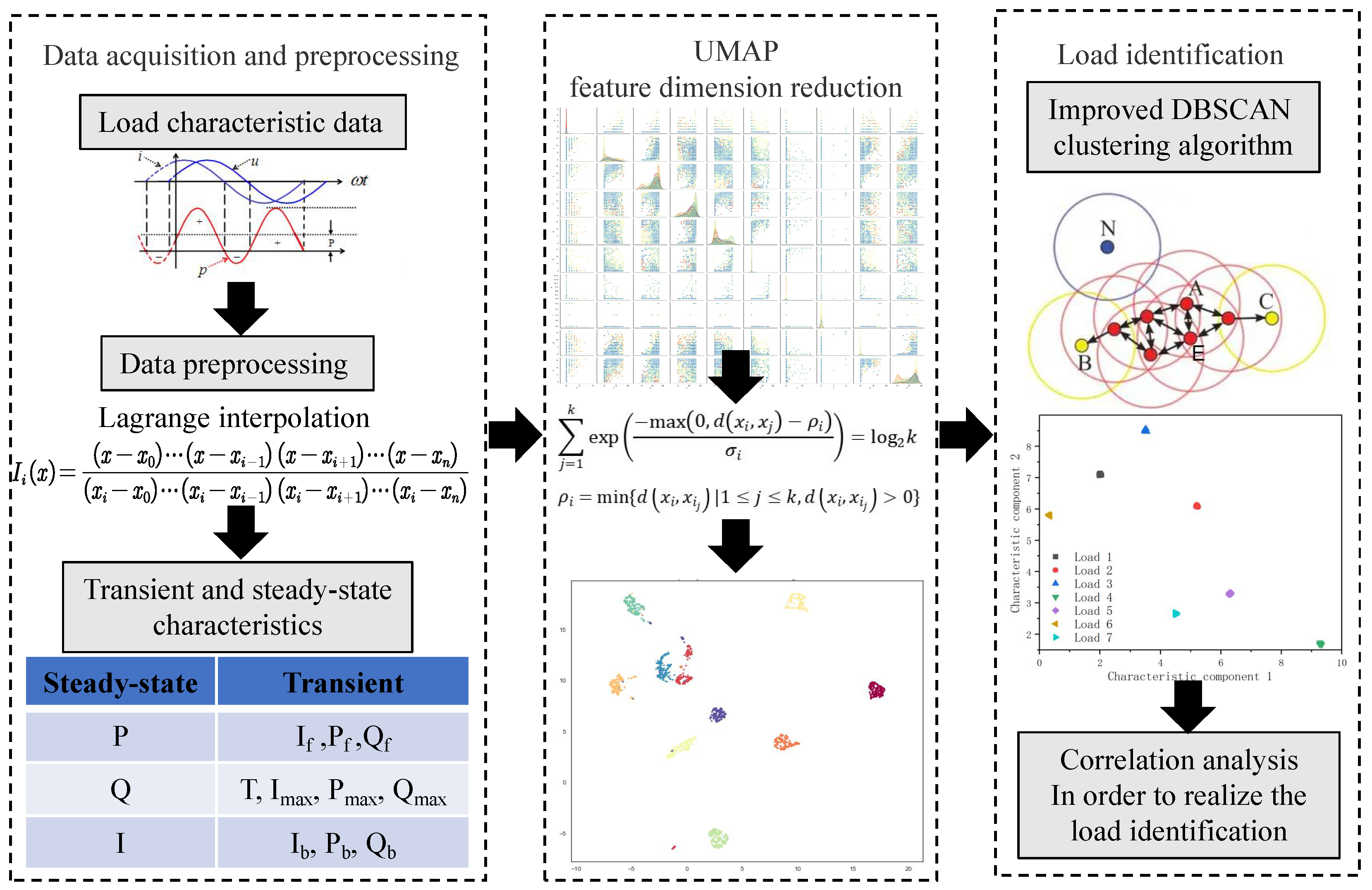
This paper presents an effective load identification method. By using the UMAP dimensionality reduction algorithm to reduce the selected feature data, the load feature template library is constructed. Then, the improved DBSCAN clustering algorithm is used to realize sample clustering in the template library, and the Euclidean distance between the load to be identified and the cluster center of the template library is calculated to determine the load to be identified.

(2)

To overcome the problem of information redundancy caused by excessive load feature dimension, the UMAP algorithm is applied in load feature dimensionality reduction to reduce data correlation and maximize the characterization of payload characteristics.

(3)

To improve the accuracy of load identification, we propose an improved DBSCAN clustering method to cluster the feature data in the load feature database and realize load type matching.

The rest of this paper is arranged as follows. A NILM method based on uniform popular approximation and projection (UMAP) reduction and improved DBSCAN clustering is proposed in Section 2. The principles of the UMAP load feature dimensionality reduction algorithm and DBSCAN clustering are introduced, respectively, and the overall framework is discussed. In Section 3, the simulation examples are carried out to analyze the proposed method based on the user’s electricity consumption data in the CER–Electricity–Data dataset, and the common load data of a user in Zhejiang Province in China are used as a practical example to verify the load recognition algorithm. Section 4 summarizes this work.

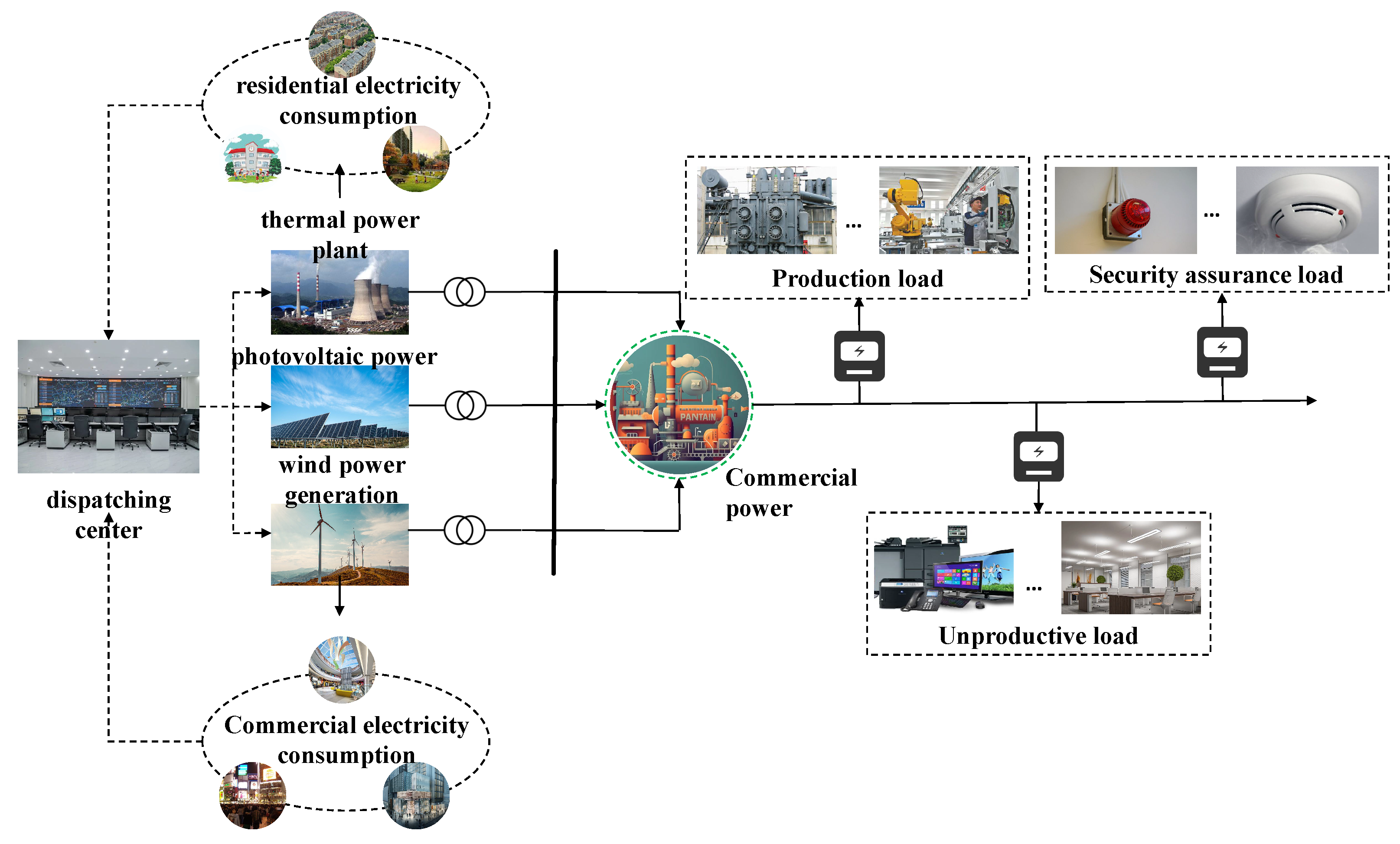
2. Analysis of User Side Load Characteristics

As shown in Figure 1, user characteristics form the basis of load identification. There are various types of electricity loads on the user side, and the electrical signal characteristics of different load types also vary. The electricity consumption data of users are essentially a time series [47,48,49]. By analyzing and modeling the trend of this time series, its inherent rules and characteristics can be analyzed. The side load electricity consumption of industrial user equipment has the following general characteristics:

• The load current will show obvious fluctuation characteristics with time;
• When the load is put in and cut out, the instantaneous current will change obviously;
• After the load is switched between working and stopping states, the current waveform on the user side and power line is considered stable.

Based on the above three assumptions, after a load input or load interruption event, power users will go through three stages: transient during the switch-on stage, a stable stage, and transient after switching off. The pre-transient stage represents the original steady state of the power load before switch-on or shutdown, while the post-transient stage represents the steady state of the power load after switch-on or shutdown. For the scenario of power load identification, we need to extract the electrical signal characteristics of the power load in both steady-state and transient processes separately. This kind of load switching event, that is, the extraction of steady-state process features and transient process features of the load, usually requires an event detection algorithm to monitor the operation process of load in real time to obtain the load switching event point and finally obtain the corresponding load characteristics. The specific implementation steps are shown in [16].

2.1. Steady-State Feature Extraction of User Load

Usually, the active and reactive power of the load under stable operating conditions are selected as characteristic indicators due to the cyclical nature of user-side load work [50]. Considering actual power scenarios, it is often convenient to obtain power and current signals. In order to comprehensively describe the power consumption characteristics of electrical loads, as shown in

Table 2. Steady-state characteristics of user load.

Sequence Number	Characteristic Index
1	Active power (P)
2	Reactive power (Q)
3	RMS value of current (I)

, this paper still uses active power, reactive power, and root mean square (RMS) values under stable operating conditions as load characteristic indicators.

2.2. User Load Transient Feature Extraction

To identify the transient process of power loads, it is necessary to first detect the initial event of the transient process and then capture the reactive power, active power, and current waveforms of the transient process as transient characteristic samples of power loads. In order to comprehensively describe the transient process of power loads, this paper selects the characteristic variables of the three stages before, during, and after the transient occurrence that power loads go through during the input and output stages. In order to adapt to the proposed NILM algorithm, this paper constructs a comprehensive load characteristic space for transient processes. As shown in

Table 3. Three states of user load and 10 characteristic indicators.

Transient Process	Characteristic Index
Before transient	RMS of current $I_f$
	Mean active power $P_f$
	Mean reactive power $Q_f$
During transient	Transient duration T
	Maximum current $I_{max}$
	Maximum active power $P_{max}$
	Maximum reactive power $Q_{max}$
After transient	RMS of current $I_b$
	Mean active power $P_b$
	Mean reactive power $Q_b$

, this paper lists a total of 10 functional labels.

Specifically, we can first obtain N cycles of instantaneous current $I_n=\left\{I_1,I_2,\dots ,I_N\right\}$ and instantaneous voltage $U_n=\{U_1,U_2,\dots ,U_N\}$ in the data acquisition process, where $n=\left\{1,2,\dots ,N\right\}$. The instantaneous current in a single period can be expressed as $I=\left\{i_1,i_2,\dots ,i_m\right\}$, and the instantaneous voltage can be expressed as $U=\left\{u_1,u_2,\dots ,u_m\right\}$, where $m=f_1/f_2$, $f_1$ is the data acquisition frequency, $f_2$ is the power frequency of the collection site (50 Hz or 60 Hz), and m represents the number of data samples in a single cycle. Thus, the effective current values $I_f$ and $I_b$ before and after the transient state can be obtained as follows:

$$I_f=\sqrt{{\displaystyle \frac{1}{m}}{\int }_0^{m}I{\left(t\right)}^{2}dt},$$

(1)

$$I_b=\sqrt{{\displaystyle \frac{1}{m}}{\int }_0^{m}I{\left(t\right)}^{2}dt}.$$

(2)

According to the formula $P\left(t\right)=I\left(t\right)\times U\left(t\right)$, the instantaneous power of a single cycle $p=\left\{p_1,p_2,\dots ,p_m\right\}$. The active power P of a single period is the average instantaneous power p, usually obtained by calculating the average instantaneous power: $P={\displaystyle \frac{1}{m}}{\int }_0^{m}p\left(t\right)dt$. The reactive power Q of a single period can be obtained by calculating the square variance of apparent power S and active power P: $Q=\sqrt{S^2-P^2}$, where $S={\displaystyle \frac{1}{m}}{\int }_0^m\left|p\left(t\right)\right|dt$.

Based on this, we can obtain the active power of N cycles $P_n=\left\{P_1,P_2,\dots ,P_N\right\}$ and the reactive power of N cycles $Q_n=\left\{Q_1,Q_2,\dots ,Q_N\right\}$. The average active power and average reactive power of the first N cycles of the transient state can be expressed as follows:

$$P_f={\displaystyle \frac{1}{N}}\sum _{n=N}{P}_n,$$

(3)

$$Q_f={\displaystyle \frac{1}{N}}\sum _{n=N}{Q}_n,$$

(4)

where $P_n$ and $Q_n$ are the active power and reactive power of the Nth cycle before the transient state.

At the same time, we can obtain the average active power and average reactive power of N cycles after the transient state, which can be expressed as follows:

$$P_b={\displaystyle \frac{1}{N}}\sum _{n=N}{P}_n,$$

(5)

$$Q_b={\displaystyle \frac{1}{N}}\sum _{n=N}{Q}_n,$$

(6)

where $P_n$ and $Q_n$ are active power and reactive power in the Nth cycle after the transient state.

To solve the maximum active power P_max and maximum reactive power Q_max in the transient process, the active power $P_n$ and reactive power $Q_n$ in N cycles in the transient process need to be obtained through the above steps. Therefore, the following applies:

$$P_{max}=max\left\{P_n=\left\{P_1,P_2,\dots ,P_N\right\}\right\},$$

(7)

$$Q_{max}=max\left\{Q_n=\left\{Q_1,Q_2,\dots ,Q_N\right\}\right\}.$$

(8)

The maximum current of N cycles in the transient process can be defined as follows:

$$I_{max}=max\left\{max\left\{I_1\right\},max\left\{{\mathrm{I}}_2\right\},\dots ,max\left\{{\mathrm{I}}_{\mathrm{N}}\right\}\right\}.$$

(9)

Specifically, load feature extraction refers to the extraction of sequence data corresponding to various load features in the constructed feature space. The categories of load features contained in the feature space are shown in Table 2 and Table 3. For example, to extract the load characteristics of the luminaire, it is necessary to obtain the individual characteristics of the appliance, such as the transient active power series, the transient reactive power series, and the transient current series. Combining the sequence data of these individual features, the feature space is constructed to realize the load feature extraction of the device. The sequence data of each single load feature extracted in the process of load feature extraction can be understood as load feature data. In this paper, the sequence data corresponding to 13 load features selected from Table 2 and Table 3 are the load feature data. Through these load feature data, load feature space can be constructed to realize load feature extraction.

3. Proposed Load Identification Method

In the actual industrial scenario, industrial load data has difficulty in data collection, small data sample size, and high data feature dimension [51]. Therefore, this paper adopts the UMAP dimensionality reduction algorithm and DBSCAN feature clustering method for load identification. Compared with existing CNNs, gated recurrent units (GRUs), recurrent neural networks (RNNs), long short-term memory networks (LSTMs), and time convolutional networks (TCNs), these deep networks require a large number of samples and consume higher training resources. The demand for data samples of clustering algorithms is quite low, and the load identification accuracy based on limited samples is high.

According to the analysis and extraction of user electricity characteristics, the transient characteristics and steady-state characteristics of the load are reduced by the UMAP method, and a new load characteristic data domain is constructed. Then, the DBSCAN method is utilized to classify the common user load events and further identify which kind of load occurs in the switching action. The correlation analysis is performed between the identified load and the data template to identify the load type more accurately.

3.1. Dimension Reduction of UMAP Feature Data

Excessive load feature dimension will not only increase the calculation amount of the load identification algorithm but also lead to incorrect identification results due to redundant information among load features. As nonlinear data, a nonlinear dimensionality reduction algorithm is needed for load characteristic data. The existing nonlinear dimensionality reduction methods can be divided into two types. One is a kernel-based dimensionality reduction algorithm, which maps nonlinear data to a high-dimensional kernel space through kernel functions, allowing the original data to be separated and compressed in the high-dimensional space. Kernel principal component analysis (KPCA) [52] is a typical dimensionality reduction algorithm based on the kernel method. The other is the dimensionality reduction method based on manifold learning, which achieves the problem of dimensionality reduction for high-dimensional data from the perspective of data morphology. The representative methods include local linear embedding (LLE) [53], isometric mapping (ISOMAP) [54], t-distributed stochastic neighbor embedding (t-SNE) [55], etc. Compared with the dimensionality reduction effect of each algorithm for the load multidimensional feature data set, the UMAP dimensionality reduction algorithm can distinguish different load types more prominently, with less aliasing and clear distinction boundaries. The UMAP algorithm has the best dimensionality reduction performance, so it was chosen as the fitting dimensionality reduction method to reduce the load feature dataset, preparing for subsequent load identification.

To decrease the influence of redundant load characteristic information, this paper first uses the UMAP dimensionality reduction algorithm to extract and reduce the payload characteristics. UMAP was proposed in 2018 and was created using the theory of algebraic topology and Riemannian geometry to reduce the dimension of data samples while preserving the global structural characteristics of the data as much as possible.

Let $X=\left\{x_1,x_2,\dots ,x_N\right\}$ be the input data set for any $x_i$ definition ${\rho }_i$ and ${\sigma }_i$:

$${\rho }_i=min\left\{d\left(x_i,x_j\right)\left|1\le j\le k,d\left(x_i,x_j\right)>0\right.\right\},$$

(10)

$${log}_{2}k=\sum _{j=1}^{k}exp\left({\displaystyle \frac{-max\left(0,d\left(x_i,x_j\right)-{\rho }_i\right)}{{\sigma }_i}}\right),$$

(11)

where ${\sigma }_i$ is the length scale parameter, and ${\rho }_i$ represents a point with an edge weight of 1, which is connected to $x_i$.

Defining a directed weighted graph satisfies the condition of $\overline{G}=\left(V,E,w\right)$, and the symmetry of $\overline{G}$ is selected to define the undirected weighted graph G. Assuming that the weighted adjacency matrix of weighted graph G is A, the symmetric matrix can be obtained as follows:

$$B=A+A^T-A\otimes A^T.$$

(12)

The undirected weighted neighborhood graph G can be defined through the adjacency matrix B and ⊗ is the Hadamard product. The UMAP applies attractive and repulsive forces along boundaries and vertices, respectively. To evaluate an equivalent weighted graph H obtained from $\left\{y_i\right\},i=1,2,\dots ,N$, the gravitational forces $F_{gr}$ of i and j at coordinates $y_i$ and $y_j$ can be expressed as follows:

$$F_{gr}={\displaystyle \frac{-2b{\parallel y_i-y_j\parallel }_2^{2\left(b-1\right)}}{1+{\parallel y_i-y_j\parallel }_2^2}}\omega \left(x_i,x_j\right)\left(y_i-y_j\right),$$

(13)

where b denotes the hyper-parameters. The repulsive force $F_{re}$ can be given as follows:

$$F_{re}={\displaystyle \frac{2b\left[1-\omega \left(x_i,x_j\right)\right]\left(y_i-y_j\right)}{\left(\epsilon +{\parallel y_i-y_j\parallel }_2^2\right)\left(1+a{\parallel y_i-y_j\parallel }_2^{2b}\right)}},$$

(14)

where $\epsilon$ denotes a small value to prevent the denominator from being equal to 0. This paper uses cross-entropy to calculate the difference between G and H. With this difference value, the topology of original data can be matched, thereby obtaining a low dimensional output of the data. This paper selects the RMS of the current, active power, and reactive power of the power load in a steady state as characteristic data. In addition, based on the stable operating characteristics of power loads, as shown in Table 2, this paper introduces 10 sets of features (such as $I_f$, $P_f$, $Q_f$, T, I_max, P_max, Q_max, $I_b$, $P_b$, and $Q_b$), which together form a 13-dimensional feature vector for the input features.

It is worth noting that as a load identification scheme, the resolution of the data used in the proposed method is mainly determined by the resolution of the selected load feature data. The load features selected in this paper combine transient and steady-state characteristics, which belong to high-frequency characteristics (>1 kHz), and the resolution of the data used to obtain the complete load characteristics must be greater than 1 kHz.

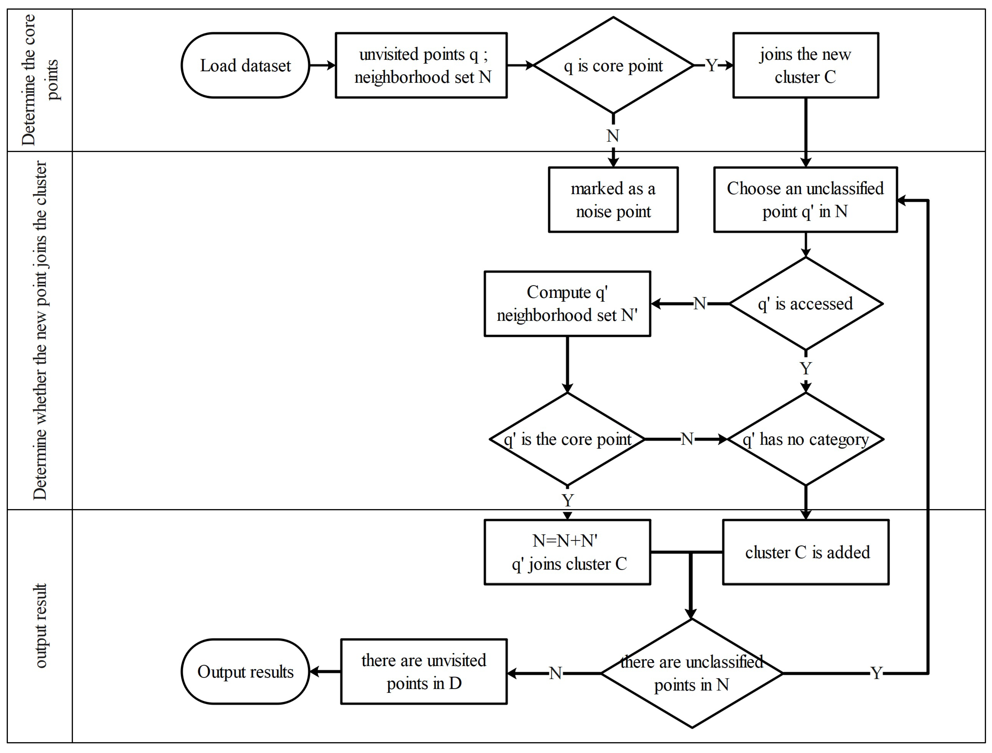
3.2. DBSCAN Feature Clustering Method

Unlike existing K-means clustering algorithms, K-means is often suitable for sample sets with flat clustering geometry, a small number of clusters, or relatively similar feature sizes. The DBSCAN clustering algorithm used in this paper is suitable for datasets with density differences between samples [56]. The principle of DBSCAN clustering is to define the areas of the remaining samples with significantly higher data density than the average density of the sample set as clusters while defining the low-density areas of the samples as the boundaries of the clusters. The advantage of doing so is to distinguish different clusters based on data density, which is not affected by sample shape and dimension. The workflow of DBSCAN clustering proposed in this paper can be explained as follows:

DBSCAN operates through a series of local regions to characterize the proximity of the dataset, with parameters ($ϵ$, $MinPts$) defining the degree of clustering within these regions. In this paper, $ϵ$ represents the radius threshold for a given sample’s vicinity, while $MinPts$ denotes the minimum count of samples within that vicinity at a distance of $ϵ$. Given a dataset $D=\{x_1,x_2,\dots ,x_m\}$, the precise density characterization of DBSCAN is formulated as follows.

• $ϵ$-neighborhood: For $x_jϵD$, its $ϵ$-neighborhood contains the subsample set in the sample set D whose distance from $x_j$ is not greater than $ϵ$, and the number of this subsample set is denoted as $\left|Nϵ\left(x_j\right)\right|$; that is, $Nϵ\left(x_j\right)=\left\{x_i\in D\left|distance\left(x_i,x_j\right)\le ϵ\right.\right\}$.
• Core object: For any sample $x_j\in D$, $x_j$ is a core object if its $ϵ$-neighborhood corresponding to $Nϵ\left(x_j\right)$ contains at least $MinPts$ samples; that is, $Nϵ\left(x_j\right)\left|\ge MinPts\right.$.
• Density direct: If point $x_i$ falls within an $ϵ$-radius of point $x_j$ and $x_j$ is recognized as a central element, we consider $x_i$ to be density-reachable from $x_j$. However, the reverse implication does not hold universally. $x_i$ is density-reachable from $x_j$, and it does not automatically mean that $x_j$ is density-reachable from $x_i$. This only becomes true if $x_i$ itself is also identified as a central element.
• Density-reachable: Consider two points $x_i$ and $x_j$. If a sample sequence $p_1,p_2,\dots ,p_t$ is found such that $p_1$ corresponds to $x_i$, $p_T$ corresponds to $x_j$, and each $p_{t+1}$ is derived directly from its preceding point in density terms, we can say that $x_j$ is density-reachable from $x_i$ [57]. This indicates that density reachability exhibits the property of transitivity. It is important to highlight that all intermediate samples $p_1,p_2,\dots ,p_{T-1}$ in this sequence must be core objects; this is due to the fact that only core objects have the capability to influence the density of other samples directly. Additionally, it is worth noting that density reachability does not uphold the principle of symmetry, which can be attributed to the inherent asymmetry observed in density direct reachability.
• Density-connected: For sample points $x_i$ and $x_j$, if there exists a core object sample $x_k$ such that both $x_i$ and $x_j$ can reach density through $x_k$, then we say that $x_i$ and $x_j$ are density-connected. This density relationship is symmetric.

The key to DBSCAN lies in setting a distance threshold $\epsilon$ and a minimum number of points threshold $MinPts$. Setting these two parameters too large or too small will affect the clustering effect. Therefore, appropriate values of $\epsilon$ and $MinPts$ should be selected according to the distribution characteristics of the given data set. Through the understanding of the distribution characteristics of the data set, the values of these two parameters can be reasonably selected so as to obtain better clustering results. This paper adopts a quantitative calculation method, considering the distance between the monitored sample and local data density, to calculate the Euclidean distance $d_{ij}$, ${\rho }_i$, cut-off distance $d_c$, and $MinPts$, which can be expressed as follows:

$${\rho }_i=\sum _{i=1}^{n}L\left(d_{ij}-d_c\right),i\ne j,$$

(15)

$$d_c=mean\left(d_y\right),$$

(16)

$$MinPts=round\left(mean\left({\rho }_i\right)\right),$$

(17)

$$d_{ij}=\sqrt{{\sum }_{i=1}^n{\sum }_{j=1}^n{\left(x_i-x_j\right)}^2},$$

(18)

where $d_{ij}$ represents the Euclidean distance between two data $x_i$ and $x_j$ [58], $d_c$ is the cut-off distance, and $L\left(d_{ij}-d_c\right)$ is the binary function. If $d_{ij}<d_c$, then $L\left(d_{ij}-d_c\right)=1$, otherwise 0.

From Equation (9), it can be seen that compared to $d_c$, the local density of $x_i$ is closer to $x_i$, and $rh{o}_i$ represents how many points are closer to $x_i$. In addition, Equation (10) indicates that the value of the cut-off distance is determined by the average distance between all the data, and the $MinPts$ obtained is the average of the number of fields and then rounded. After determining the $MinPts$, the domain radius needs to be determined. Ankerst et al. proposed a neighborhood radius calculation for considering $MinPts$ and the volume of the hypersphere around all data. Assuming an n-dimensional data set $D=\left\{x_i,\dots ,x_i,\dots ,x_m\right\}$, the formula is as follows:

$$\epsilon =\sqrt[n]{{\displaystyle \frac{V_D\times MinPts\times \Gamma \left(\frac{n}{2}+1\right)}{m\times {\pi }^{n/2}}}}{V}_D^{hs}={\displaystyle \frac{{\pi }^{\frac{n}{2}}}{\Gamma \left(\frac{n}{2}+1\right)}}{r}^n,$$

(19)

where $V_D^{hs}$ represents the volume of the hypersphere, $\Gamma$ denotes the Gamma function, and r represents the radius of the sphere. This method uses the concept of the hypersphere, but there are some shortcomings; that is, although the constructed hyperconvex bread contains all data points, the spatial distribution is irregular, and the data density is uneven, resulting in a domain radius of $\epsilon$ that may be too large, which poses great difficulties for subsequent calculations. Therefore, a simpler and more suitable method for obtaining the domain radius is proposed, and the formula is as follows:

$$V_D={\prod }_1^n{\displaystyle \frac{max\left(x^1\right)+min\left(x^1\right)}{2}},$$

(20)

where $max\left(x^1\right)$ and $min\left(x^1\right)$ denote the maximum and minimum value in the L-th dimension, respectively. In this way, it can not only ensure that the radius $\epsilon$ of the domain is not too large, but also contain all the data, and the calculation is simpler. Therefore, the final formula for determining the radius $\epsilon$ of the domain is as follows:

$$\epsilon =\sqrt[n]{{\displaystyle \frac{V_D\times MinPts\times \Gamma \left(\frac{n}{2}+1\right)}{m\times {\pi }^{n/2}}}},$$

(21)

where $V_D={\prod }_1^n{\displaystyle \frac{max\left(x^1\right)+min\left(x^1\right)}{2}}$. The flow chart of DBSCAN feature clustering algorithm is shown in Figure 2.

3.3. UMAP Dimensionality Reduction and Adapted DBSCAN Clustering

The NILM method based on UMAP dimensionality reduction and adapted DBSCAN clustering proposed in this paper is shown in Figure 3. Upon detection of a load input and output event, we proceed to extract the relevant load characteristics and reduce their dimensionality, taking into account the load current waveform. To enhance the accuracy of load identification, we employ a dual approach that integrates both unsupervised DBSCAN load clustering and supervised association analysis for load identification. Our methodology involves utilizing the DBSCAN algorithm to categorize sample data with known equipment labels from our load feature template library. By identifying the cluster centers, we then compute the Euclidean distance between the unidentified load and these centers within the feature template library. This process yields a load feature-matching outcome based on the magnitude of the Euclidean distance values. Moreover, to bolster the dependability of the outcomes pertaining to load identification, it is essential to take into account the holistic attributes of the load. A thorough correlation examination is employed to gauge the interrelation between the traits of the load under scrutiny and those present within the reference library of load characteristics. The higher the aggregate correlation score, the greater the resemblance between the load in question and potential electrical counterparts, thereby facilitating the accomplishment of load type alignment. Drawing upon the aforementioned methodology for assessing load characteristics, the present study has developed a NILM approach that integrates the UMAP dimensionality reduction technique with the DBSCAN clustering algorithm.

4. Example Analysis

4.1. Evaluation Indicators

To evaluate the effect of load identification, the identification accuracy ($Acc$), $Precision$, $Recall$, and $F1$ score are selected as the algorithm evaluation indicators [59] to represent the accuracy of load decomposition, which are defined as follows:

$$Acc={\displaystyle \frac{TP+TN}{TP+TN+FP+FN}},$$

(22)

$$Precision={\displaystyle \frac{TP}{TP+FP}},$$

(23)

$$Recall={\displaystyle \frac{TP}{TP+FN}},$$

(24)

$$F1={\displaystyle \frac{2\times Precision\times Recall}{Precision+Recall}},$$

(25)

where $TP$ is the true positive, and the true value is judged as a positive class. $FP$ is the false positive, and the true value is judged as a negative class, which is judged as positive class. $TN$ is the true negative, and $TP$ is the true positive class. Anything with a negative true value is classified as a negative class. $FN$ is classified as a false negative, and anything with a positive true value is classified as a negative class.

4.2. Example Analysis

4.2.1. Case I: A Simulation Example

In this paper, in order to verify the performance of the method in this paper, the simulation device is a Lenovo PC, the operating system is a Windows10 64-bit ultimate edition, with an Intel i52450mCPU, the frequency is 2.5 GHz, with 8 GB memory, and a Python3.8 environment. Seven types of loads commonly used by industrial users in the CER–Electricity–Data dataset [60] are selected, data pre-processing is carried out according to the characteristic data, and then the load identification model is trained and tested. The specific information of the seven loads selected is shown in

Table 4. Selected load-specific information.

Load Number	Load Class
Load 1	Lighting
Load 2	Fan
Load 3	Electric control cabinet
Load 4	Motor
Load 5	Air conditioning
Load 6	Compressor
Load 7	Cleaning machine

. In order to ensure the universality of the model, this paper also uses seven kinds of electrical equipment loads of a family in the PLAID dataset to train and test the load identification model. We use the Erada rule to eliminate random error data and get relatively accurate data. According to Nyquist’s theorem [61], downsampling and processing of 10 kHz data at 1 kHz frequency not only reduces the requirements of the system for sampling equipment but also improves the efficiency of data pre-processing. The downsampled data do not affect the load feature extraction, and the amount of data are reduced to one-tenth of the original.

The UMAP algorithm serves as a tool to streamline both the steady-state and transient attributes of various loads into a more manageable form. Given the substantial volume of data resulting from the comprehensive dimensionality reduction process, a focused examination is conducted on the dimensionality reduction outcomes pertaining to the seven specific load categories under review. In this paper, 13 kinds of power load steady-state and transient characteristics are selected as the feature database. After feature dimensionality reduction through UMAP, a low-dimensional feature database containing transient and steady-state characteristics of power load is constructed to facilitate cluster analysis and sample center setting. Post-UMAP processing, these seven types of loads are simplified into two-dimensional representations according to the load feature library constructed in Section 1, as depicted in Figure 4. Notably, following this reduction, distinct clusters emerge among the characteristic elements of diverse electrical devices, showcasing clear distinctions between categories. This strategic simplification not only alleviates the computational demands associated with load classification but also bolsters the overall efficacy of the identification process.

After dimensionality reduction through UMAP, the 13-dimensional feature library constructed by us has been simplified to a two-dimensional feature form, and each sample containing the 13-dimensional feature library is correspondingly simplified to a two-dimensional feature sample. DBSCAN was used to cluster these two-dimensional feature samples to build seven cluster centers to represent seven kinds of loads. The clustering results are shown in Figure 5. It can be observed from Figure 5 that DBSCAN clustering can effectively separate the feature samples of the same electrical devices in the load feature database and distribute them more closely in the dimensionality reduction feature space. It can be seen that the feature clustering of different electrical equipment has clear boundaries and a small overlap in the feature space, which is conducive to subsequent load feature matching. In order to quantify the similarity of each feature in the target load feature database, the clustering centers of the target load under a steady state and transient state are given. This has the advantage of helping to obtain the Euclidean distance between the cluster center and the reference sample in the target load, as shown in

Table 5. Clustering centers of steady-transient load characteristics.

Load Name	Steady-State Feature Cluster Centers		Transient Feature Cluster Centers
	Characteristic Component 1	Characteristic Component 2	Characteristic Component 1	Characteristic Component 2
Load 1	0.082	0.054	0.083	0.032
Load 2	0.084	−0.032	0.046	−0.021
Load 3	−0.078	−0.071	−0.082	−0.026
Load 4	0.083	0.049	0.068	−0.054
Load 5	−0.104	−0.058	−0.098	0.042
Load 6	−0.066	−0.068	−0.054	−0.024
Load 7	0.075	−0.027	0.063	−0.035

.

When there is a new set of switching events to be identified, the algorithm in this paper extracts the corresponding feature index, constructs the sample to be processed, including a 13-dimensional feature library through the same normalization process, and then simplifies the sample to a two-dimensional form through the UMAP algorithm. The DBSCAN clustering algorithm can obtain recognition results according to the Euclidean distance between the cluster center set above and the two-dimensional detection. By using the CER–Electric–Data dataset, we can construct 1000 samples containing 13-dimensional feature libraries for seven kinds of loads, respectively. The load identification method we proposed can be used to obtain the identification results of each of the seven loads, as shown in

Table 6. Results evaluation of load identification.

Loads	Accuracy	Precision	Recall	F1-Score
Load 1	93.8%	92.8%	89.2%	91%
Load 2	96.5%	93.5%	94.5%	94%
Load 3	92.6%	91.7%	91.2%	91.4%
Load 4	97.4%	93.4%	90.4%	91.9%
Load 5	96.7%	94.2%	93.3%	93.7%
Load 6	94.3%	90.6%	91.6%	91.6%
Load 7	95.8%	95.2%	93.8%	94.5%
Total	95.3%	93.1%	92%	92.5%

.

The CER–Electricity–Data dataset is used to verify the working effect of the proposed method in industrial scenarios. In order to show the generalization of the model in this paper, seven typical household load data in PLAID datasets are used to verify the model, and the results are shown in

Table 7. Identification results of the model under the PLAID dataset.

Loads	Accuracy	Recall	F1-Score
Electric fan	91%	97%	91%
Electric hair drier	92%	99%	93%
Incandescent light bulb	95%	98%	94%
Refrigerator	95%	99%	94%
Air conditioner	97%	99%	98%
Washing machine	96%	97%	96%
computer	96%	96%	96%
Total	94.5%	97.8%	94.5%

. It can be seen that this model still has a good effect on the identification of household loads.

To assess the efficacy of the load identification algorithm introduced in this study, a comparative analysis was conducted using four distinct methodologies: wavelet transformation, decision tree modeling, backpropagation (BP) neural networks, and PCA-BDBSCAN, t-SNE-DBSCAN, and UMAP-K-means convolutional neural network (CNN) algorithms. These methods are employed for identifying loads, and their respective error rates are juxtaposed against those yielded by the algorithm detailed in our research. As evidenced by the data presented in

Table 8. Comparative analysis of load identification results using different methods.

Comparison Method	Accuracy (%)
Wavelet transform [62]	88.5
Decision tree model [63]	89.6
BP neural network	90.8
CNNs	91.6
PCA-DBSCAN	90.4
t-SNE-DBSCAN	92.8
UMAP-K-means	89.5
Ours	95.3

, the accuracy of load identification achieved through the novel approach notably surpasses that of the alternative algorithms under examination.

4.2.2. Case II: A Practical Example

In this paper, the power load data of an industrial scene in a certain area of Zhejiang Province is selected for power load identification; firstly, the collected load data are pre-processed, and the conditional average method is used to replace the missing or abnormal data. Then, the load data characteristics are analyzed, and seven common user loads are selected. Each load has two transient processes: input and removal. Following this, the UMAP algorithm is employed to separately decrease the dimensions of both the steady-state performance and the transient behavior of electrical loads. The outcomes of this dimensional reduction process, specifically applied to the characteristic profiles of the seven distinct load categories previously outlined, are then subjected to a comprehensive examination.

After UMAP dimensionality reduction of load characteristics, load characteristics are reduced to two dimensions. Finally, the load feature template library after dimension reduction is used for DBSCAN clustering, and the feature samples of the same electrical equipment are clustered by DBSCAN, which could form better clusters. The subsequent implementation of feature matching for load analysis demonstrates enhanced capabilities in accurately identifying load characteristics. Herein lie the empirical findings that substantiate this improvement.

As can be seen from Figure 6, DBSCAN clustering of actual user electricity load data feature samples after feature dimension reduction can also form good clusters, which can ensure the accuracy of subsequent load feature matching.

Table 9. Results evaluation of load identification.

Load	Accuracy	Precision	Recall	F1 Score
Load 1	96.3%	93.9%	94.2%	94%
Load 2	95.5%	92.6%	93.1%	92.8%
Load 3	96.5%	93.7%	93.8%	93.7%
Load 4	94.9%	92.4%	91.4%	91.9%
Load 5	92.4%	90.3%	91%	90.6%
Load 6	92.7%	89.8%	90.6%	90.2%
Load 7	95.1%	92.7%	91.8%	92.2%
Total	94.8%	92.2%	92.3%	92.2%

shows the actual load identification results. From the table, we can see that the average accuracy rate is approximately 94.8%, the accuracy of the lowest load identification type can also reach 92.4%, and other indicators also have good performance. It is known that even the actual load data can also have a high identification accuracy rate. The validity of this method is further validated.

From the above experimental results, it can be seen that the load identification method of UMAP-DBSCAN has good performance. The main reason is that DBSCAN can deal with clusters of arbitrary shape and identify noise, while UMAP enhances the separability of clusters by optimizing the embedding vector so that even when the clusters have complex shapes, uneven densities, or overlaps, the load identification method of UMAP-DBSCAN has good performance. Clustering can also be carried out efficiently. In the NILM domain, the combination of UMAP and DBSCAN can simplify the problem because the topological preprocessing of UMAP reduces the need for DBSCAN parameter tuning while improving the accuracy and reliability of clustering. The adaptive nature of UMAP enables it to deal with clusters of different densities, while DBSCAN is able to identify these clusters and separate them, which is especially important for handling various electrical load patterns in NILM.

5. Conclusions

NILM provides a robust basis for energy management by accurately identifying each electrical appliance in the user’s electricity consumption. Its advantage is that it can optimize energy distribution, and its importance is taken into account in the construction of energy conservation, emission reduction, and smart home systems. The multitude of load varieties and the extensive range of load characteristics present considerable challenges in managing data handling and ensuring accurate feature alignment during load recognition processes. In response to these issues, this study introduces an innovative approach to non-intrusive load detection that leverages the dimensionality reduction capabilities of UMAP combined with an enhanced version of DBSCAN. In the initial step, our approach involves a meticulous analysis and preprocessing of energy consumption data, culminating in the establishment of a comprehensive load feature database. Subsequently, we employ the UMAP to reduce the complexity of high-dimensional data and streamline the load features. This dimensional reduction process allows for the reconfiguration of the load feature database, making it more manageable and accessible for subsequent analyses or applications. Finally, through the improved DBSCAN clustering algorithm, the load characteristics are analyzed, and the load types are matched. To validate the effectiveness of the proposed method, the CER–Electricity–Data dataset and the load data of a region in Zhejiang Province in China are used only for verification. The accuracy rate is presented as an evaluation index and compared with the existing wavelet transform decision tree model, BP neural network, and CNN algorithms, and the accuracy rate of the proposed method reaches 95.3%. The results of multiple groups of experiments show that our method has a significant improvement in all evaluation criteria, which further proves the superiority of our method. However, this paper only sets examples to verify the proposed load identification method and fails to integrate the method and upload it to the cloud to realize real-time load identification. In the next research, we will obtain the load characteristic data at the client side through cloud collaboration and upload it to the load identification model block after cloud integration to realize the load identification on the cloud.

References

1. Wang, D.; Jiang, Y.; Qiu, C.; Xiong, H.; Bi, M.; Ge, Y.; Li, J.; Cao, Y.; Li, G.; Cui, Z.; et al. Power system real time reliability monitoring and security assessment in short-term and on-line mode. In Proceedings of the 2019 IEEE Innovative Smart Grid Technologies-Asia (ISGT Asia), Chengdu, China, 21–24 May 2019; IEEE: Piscataway, NJ, USA, 2019; pp. 758–763. [Google Scholar]
2. Chen, Y.; Lao, K.W.; Qi, D.; Hui, H.; Yang, S.; Yan, Y.; Zheng, Y. Distributed Self-Triggered Control for Frequency Restoration and Active Power Sharing in Islanded Microgrids. IEEE Trans. Ind. Inform. 2023, 19, 10635–10646. [Google Scholar] [CrossRef]
3. Chen, Y.; Qi, D.; Hui, H.; Yang, S.; Gu, Y.; Yan, Y.; Zheng, Y.; Zhang, J. Self-triggered coordination of distributed renewable generators for frequency restoration in islanded microgrids: A low communication and computation strategy. Adv. Appl. Energy 2023, 10, 100128. [Google Scholar] [CrossRef]
4. Song, D.; Yang, Y.; Zheng, S.; Deng, X.; Yang, J.; Su, M.; Tang, W.; Yang, X.; Huang, L.; Joo, Y.H. New perspectives on maximum wind energy extraction of variable-speed wind turbines using previewed wind speeds. Energy Convers. Manag. 2020, 206, 112496. [Google Scholar] [CrossRef]
5. Athanasiadis, C.; Papadopoulos, T.; Kryonidis, G.; Doukas, D. A review of distribution network applications based on smart meter data analytics. Renew. Sustain. Energy Rev. 2024, 191, 114151. [Google Scholar] [CrossRef]
6. Zhu, J.; Lu, W. Research on Converged Communication of Power Line and Wireless in Electric Power Communication System. In Proceedings of the 2021 IEEE 5th Information Technology, Networking, Electronic and Automation Control Conference (ITNEC), Xi’an, China, 15–17 October 2021; IEEE: Piscataway, NJ, USA, 2021; Volume 5, pp. 627–631. [Google Scholar]
7. Schirmer, P.A.; Mporas, I. Non-intrusive load monitoring: A review. IEEE Trans. Smart Grid 2022, 14, 769–784. [Google Scholar] [CrossRef]
8. Virtsionis-Gkalinikis, N.; Nalmpantis, C.; Vrakas, D. SAED: Self-attentive energy disaggregation. Mach. Learn. 2021, 112, 4081–4100. [Google Scholar] [CrossRef]
9. Hernández, Á.; Nieto, R.; Fuentes, D.; Ureña, J. Design of a SoC architecture for the edge computing of NILM techniques. In Proceedings of the 2020 XXXV Conference on Design of Circuits and Integrated Systems (DCIS), Segovia, Spain, 18–20 November 2020; IEEE: Piscataway, NJ, USA, 2020; pp. 1–6. [Google Scholar]
10. Hussein, N.M.; Hesham, A.M.; Rashawn, M.A. States and power consumption estimation for NILM. In Proceedings of the 2019 14th International Conference on Computer Engineering and Systems (ICCES), Cairo, Egypt, 17–18 December 2019; IEEE: Piscataway, NJ, USA, 2019; pp. 275–281. [Google Scholar]
11. Held, P.; Weißhaar, D.; Mauch, S.; Abdeslam, D.O.; Benyoucef, D. Parameter optimized event detection for NILM using frequency invariant transformation of periodic signals (FIT-PS). In Proceedings of the 2018 IEEE 23rd international conference on emerging technologies and factory automation (ETFA), Torino, Italy, 4–7 September 2018; IEEE: Piscataway, NJ, USA, 2018; Volume 1, pp. 832–837. [Google Scholar]
12. Song, D.R.; Li, Q.A.; Cai, Z.; Li, L.; Yang, J.; Su, M.; Joo, Y.H. Model Predictive Control Using Multi-Step Prediction Model for Electrical Yaw System of Horizontal-Axis Wind Turbines. IEEE Trans. Sustain. Energy 2019, 10, 2084–2093. [Google Scholar] [CrossRef]
13. Athanasiadis, C.L.; Papadopoulos, T.A.; Doukas, D.I. Real-time non-intrusive load monitoring: A light-weight and scalable approach. Energy Build. 2021, 253, 111523. [Google Scholar] [CrossRef]
14. Song, D.; Liu, J.; Yang, J.; Su, M.; Wang, Y.; Yang, X.; Huang, L.; Joo, Y.H. Optimal design of wind turbines on high-altitude sites based on improved Yin-Yang pair optimization. Energy 2020, 193, 116794. [Google Scholar] [CrossRef]
15. Virtsionis Gkalinikis, N.; Nalmpantis, C.; Vrakas, D. Variational regression for multi-target energy disaggregation. Sensors 2023, 23, 2051. [Google Scholar] [CrossRef]
16. Athanasiadis, C.; Doukas, D.; Papadopoulos, T.; Chrysopoulos, A. A scalable real-time non-intrusive load monitoring system for the estimation of household appliance power consumption. Energies 2021, 14, 767. [Google Scholar] [CrossRef]
17. Deng, X.; Zhang, C.; Peng, H.; Bi, G.; Cheng, T.; Zhang, C. Short-Term Load Forecasting for Regional Power Grids Based on Correlation Analysis and Feature Extraction. In Proceedings of the 2022 7th Asia Conference on Power and Electrical Engineering (ACPEE), Hangzhou, China, 15–17 April 2022; IEEE: Piscataway, NJ, USA, 2022; pp. 1081–1085. [Google Scholar]
18. Shen, Q.; Ren, L.; Gong, C.; Wang, H. A unified feature parameter extraction strategy based on system identification for the buck converter with linear or nonlinear loads. In Proceedings of the IECON 2016—42nd Annual Conference of the IEEE Industrial Electronics Society, Florence, Italy, 24–27 October 2016; IEEE: Piscataway, NJ, USA, 2016; pp. 388–393. [Google Scholar]
19. Fang, Y.; Liang, X.; Zuo, M.J. Effect of sliding friction on transient characteristics of a gear transmission under random loading. In Proceedings of the 2017 IEEE International Conference on Systems, Man, and Cybernetics (SMC), Banff, AB, Canada, 5–8 October 2017; IEEE: Piscataway, NJ, USA, 2017; pp. 2551–2555. [Google Scholar]
20. Tian, Y.; Wang, H.; Li, A.; Shi, S.; Wu, J. Non-intrusive load monitoring using inception structure deep learning. In Proceedings of the 2020 10th International Conference on Power and Energy Systems (ICPES), Chengdu, China, 25–27 December 2020; IEEE: Piscataway, NJ, USA, 2020; pp. 151–155. [Google Scholar]
21. Feng, T.; Duan, A.; Guo, L.; Gao, H.; Chen, T.; Yu, Y. Deep learning based load and position identification of complex structure. In Proceedings of the 2021 IEEE 16th Conference on Industrial Electronics and Applications (ICIEA), Chengdu, China, 1–4 August 2021; IEEE: Piscataway, NJ, USA, 2021; pp. 1358–1363. [Google Scholar]
22. Wei, Y.; Jin, Y.; Ju, P.; Qin, C. Identification Method of the Load Component Proportion based on the Dynamic Response under Large Disturbance. In Proceedings of the 2022 Power System and Green Energy Conference (PSGEC), Shanghai, China, 25–27 August 2022; IEEE: Piscataway, NJ, USA, 2022; pp. 824–829. [Google Scholar]
23. Song, D.; Fan, X.; Yang, J.; Liu, A.; Chen, S.; Joo, Y.H. Power extraction efficiency optimization of horizontal-axis wind turbines through optimizing control parameters of yaw control systems using an intelligent method. Appl. Energy 2018, 224, 267–279. [Google Scholar] [CrossRef]
24. Yang, Z.X.; Yu, G.; Zhao, J.; Wong, P.K.; Wang, X.B. Online Equivalent Degradation Indicator Calculation for Remaining Charging-Discharging Cycle Determination of Lithium-Ion Batteries. IEEE Trans. Veh. Technol. 2021, 70, 6613–6625. [Google Scholar] [CrossRef]
25. Wang, X.B.; Luo, L.; Tang, L.; Yang, Z.X. Automatic Representation and Detection of Fault Bearings in In-wheel Motors under Variable Load Conditions. Adv. Eng. Inform. 2021, 49, 101321. [Google Scholar] [CrossRef]
26. Chen, H.; Wang, X.-b.; Yang, Z.X. Fast Robust Capsule Network with Dynamic Pruning and Multiscale Mutual Information Maximization for Compound-Fault Diagnosis. IEEE/ASME Trans. Mechatronics 2023, 28, 838–847. [Google Scholar] [CrossRef]
27. Chen, S.; Gao, F.; Liu, T. Load identification based on factorial hidden Markov model and online performance analysis. In Proceedings of the 2017 13th IEEE Conference on Automation Science and Engineering (CASE), Xi’an, China, 20–23 August 2017; IEEE: Piscataway, NJ, USA, 2017; pp. 1249–1253. [Google Scholar]
28. Khazeiynasab, S.R.; Zhao, J.; Duan, N. WECC composite load model parameter identification using deep learning approach. In Proceedings of the 2022 IEEE Power & Energy Society General Meeting (PESGM), Denver, CO, USA, 17–21 July 2022; IEEE: Piscataway, NJ, USA, 2022; pp. 1–5. [Google Scholar]
29. Proteasa, V.A.; Ciobanu, R.I.; Dobre, C.; Marin, R.C. Federated Learning for Human Mobility. In Proceedings of the 2023 19th International Conference on Distributed Computing in Smart Systems and the Internet of Things (DCOSS-IoT), Pafos, Cyprus, 19–21 June 2023; IEEE: Piscataway, NJ, USA, 2023; pp. 780–785. [Google Scholar]
30. Wu, Z.; Fu, H. Research on load identification based on load steady and transient signal processing. In Proceedings of the 2017 10th International Congress on Image and Signal Processing, BioMedical Engineering and Informatics (CISP-BMEI), Shanghai, China, 14–16 October 2017; IEEE: Piscataway, NJ, USA, 2017; pp. 1–6. [Google Scholar]
31. Haoguang, L.; Yunhua, Y.; Xuefeng, S. Load parameter identification based on particle swarm optimization and the comparison to ant colony optimization. In Proceedings of the 2016 IEEE 11th Conference on Industrial Electronics and Applications (ICIEA), Hefei, China, 5–7 June 2016; IEEE: Piscataway, NJ, USA, 2016; pp. 545–550. [Google Scholar]
32. Iksan, N.; Udayanti, E.D.; Widodo, D.A. Time-Frequency Analysis (TFA) Method for Load Identification on Non-Intrusive Load Monitoring. In Proceedings of the 2019 4th International Conference on Information Technology, Information Systems and Electrical Engineering (ICITISEE), Yogyakarta, Indonesia, 20–21 November 2019; IEEE: Piscataway, NJ, USA, 2019; pp. 57–60. [Google Scholar]
33. Hou, S.; Lu, R.; Yang, C.; Lei, D.; Qin, W. Power system weak bus identification based on voltage distribution characteristic. In Proceedings of the 2017 IEEE Conference on Energy Internet and Energy System Integration (EI2), Beijing, China, 26–28 November 2017; IEEE: Piscataway, NJ, USA, 2017; pp. 1–6. [Google Scholar]
34. Zhi, D.; Shi, J.; Fu, R. Algorithm Implementation of Non-Intrusive Load Monitoring Based on Load Core Feature Identification. In Proceedings of the 2022 5th International Conference on Energy, Electrical and Power Engineering (CEEPE), Chongqing, China, 22–24 April 2022; IEEE: Piscataway, NJ, USA, 2022; pp. 839–844. [Google Scholar]
35. Wang, Z.; Wu, Y.; Zhao, Y.; Wang, J.; Liu, H.; Wang, Y. A Composite-Window-Based Load Event Detection Method in Non-Intrusive Load Monitoring. In Proceedings of the 2023 IEEE 7th Conference on Energy Internet and Energy System Integration (EI2), Hangzhou, China, 15–18 December 2023; IEEE: Piscataway, NJ, USA, 2023; pp. 4911–4916. [Google Scholar]
36. Ramaswamy, A.; Bal, A.; Das, A.; Gubbi, J.; Muralidharan, K.; Ramakrishnan, R.K.; Pal, A.; Balamuralidhar, P. Single feature spatio-temporal architecture for EEG Based cognitive load assessment. In Proceedings of the 2021 43rd Annual International Conference of the IEEE Engineering in Medicine & Biology Society (EMBC), Online, 1–5 November 2021; IEEE: Piscataway, NJ, USA, 2021; pp. 3717–3720. [Google Scholar]
37. Kai, D.; Zihang, H.; Shiqi, Y.; Peng, W.; Shuai, W.; Zhengmin, K. A coarse-to-fine strategy based on a supervised learning method for non-intrusive load identification. In Proceedings of the 2023 9th International Conference on Big Data Computing and Communications (BigCom), Qinghai, China, 4–6 August 2023; IEEE: Piscataway, NJ, USA, 2023; pp. 156–163. [Google Scholar]
38. Jawdat, N.; Donnal, J. Unsupervised Identification of Electrical Loads from Aggregate Power Measurements. In Proceedings of the 2022 IEEE Power & Energy Society Innovative Smart Grid Technologies Conference (ISGT), Novi Sad, Serbia, 10–12 October 2022; IEEE: Piscataway, NJ, USA, 2022; pp. 1–6. [Google Scholar]
39. Chou, P.A.; Chang, R.I. Unsupervised adaptive non-intrusive load monitoring system. In Proceedings of the 2013 IEEE International Conference on Systems, Man, and Cybernetics, Manchester, UK, 13–16 October 2013; IEEE: Piscataway, NJ, USA, 2013; pp. 3180–3185. [Google Scholar]
40. Wang, X.B.; Yang, Z.X.; Yan, X.A. Novel Particle Swarm Optimization-Based Variational Mode Decomposition Method for the Fault Diagnosis of Complex Rotating Machinery. IEEE/ASME Trans. Mechatronics 2018, 23, 68–79. [Google Scholar] [CrossRef]
41. Wang, X.B.; Yang, Z.X.; Wong, P.K.; Deng, C. Novel Paralleled Extreme Learning Machine Networks for Fault Diagnosis of Wind Turbine Drivetrain. Memetic Comput. 2019, 11, 127–142. [Google Scholar] [CrossRef]
42. Jiang, Y.; Li, C.; Yang, Z.; Zhao, Y.; Wang, X. Remaining Useful Life Estimation Combining Two-step Maximal Information Coefficient and Temporal Convolutional Network with Attention Mechanism. IEEE Access 2021, 9, 16323–16336. [Google Scholar] [CrossRef]
43. Myasnikov, E. Using UMAP for dimensionality reduction of hyperspectral data. In Proceedings of the 2020 International Multi-Conference on Industrial Engineering and Modern Technologies (FarEastCon), Vladivostok, Russia, 6–9 October 2020; IEEE: Piscataway, NJ, USA, 2020; pp. 1–5. [Google Scholar]
44. Tao, T.; Liu, Y.; Qiao, Y.; Gao, L.; Lu, J.; Zhang, C.; Wang, Y. Wind turbine blade icing diagnosis using hybrid features and Stacked-XGBoost algorithm. Renew. Energy 2021, 180, 1004–1013. [Google Scholar] [CrossRef]
45. Tao, T.; Yang, Y.; Yang, T.; Liu, S.; Guo, X.; Wang, H.; Liu, Z.; Chen, W.; Liang, C.; Long, K.; et al. Time-domain fatigue damage assessment for wind turbine tower bolts under yaw optimization control at offshore wind farm. Ocean. Eng. 2024, 303, 117706. [Google Scholar] [CrossRef]
46. Deng, D. DBSCAN clustering algorithm based on density. In Proceedings of the 2020 7th International Forum on Electrical Engineering and Automation (IFEEA), Hefei, China, 25–27 September 2020; IEEE: Piscataway, NJ, USA, 2020; pp. 949–953. [Google Scholar]
47. Yu, S.; Song, C.; Gao, P.; Zheng, H. Intelligent electricity consumption forecasting and electricity-theft analysis method based on deep learning. In Proceedings of the 2022 2nd International Conference on Electronic Information Engineering and Computer Technology (EIECT), Yan’an, China, 28–30 October 2022; IEEE: Piscataway, NJ, USA, 2022; pp. 312–316. [Google Scholar]
48. Liang, P.; Wang, W.; Yuan, X.; Liu, S.; Zhang, L.; Cheng, Y. Intelligent fault diagnosis of rolling bearing based on wavelet transform and improved ResNet under noisy labels and environment. Eng. Appl. Artif. Intell. 2022, 115, 105269. [Google Scholar] [CrossRef]
49. Liang, P.; Xu, L.; Shuai, H.; Yuan, X.; Wang, B.; Zhang, L. Semisupervised Subdomain Adaptation Graph Convolutional Network for Fault Transfer Diagnosis of Rotating Machinery Under Time-Varying Speeds. IEEE/ASME Trans. Mechatronics 2024, 29, 730–741. [Google Scholar] [CrossRef]
50. Lv, G.; Yang, Z.; Jin, Y.; Ding, Y. A novel method of complex PQ disturbances classification without adequate history data. In Proceedings of the 2016 IEEE Power and Energy Society General Meeting (PESGM), Boston, MA, USA, 17–21 July 2016; IEEE: Piscataway, NJ, USA, 2016; pp. 1–5. [Google Scholar]
51. Wang, W.; Liu, X.; Yan, L.; Yu, H.; Li, R.; Ding, N. The Software Design of Dynamic Loading Identification System of Rock Roadheader. In Proceedings of the 2017 4th International Conference on Information Science and Control Engineering (ICISCE), Changsha, China, 21–23 July 2017; IEEE: Piscataway, NJ, USA, 2017; pp. 737–740. [Google Scholar]
52. He, R.; Hu, B.G.; Zheng, W.S.; Kong, X.W. Robust principal component analysis based on maximum correntropy criterion. IEEE Trans. Image Process. 2011, 20, 1485–1494. [Google Scholar]
53. Li, R.; Liu, L. Research on rolling bearing fault diagnosis based on improved local linear embedding algorithm. In Proceedings of the 2022 Global Reliability and Prognostics and Health Management (PHM-Yantai), Yantai, China, 13–16 October 2022; IEEE: Piscataway, NJ, USA, 2022; pp. 1–3. [Google Scholar]
54. Zhang, Z.; Yu, Y.; Jiang, F.; Cheng, Q.S. Gaussian Process Regression Modeling Based on Landmark Isometric Feature Mapping for Antennas. In Proceedings of the 2021 15th European Conference on Antennas and Propagation (EuCAP), Dusseldorf, Germany, 22–26 March 2021; IEEE: Piscataway, NJ, USA, 2021; pp. 1–5. [Google Scholar]
55. Qiu, M.; Yang, Z.; Nai, W.; Li, D.; Xing, Y.; Li, K. T-distributed stochastic neighbor embedding based on cockroach swarm optimization with student distribution parameters. In Proceedings of the 2021 IEEE 12th International Conference on Software Engineering and Service Science (ICSESS), Beijing, China, 20–22 August 2021; IEEE: Piscataway, NJ, USA, 2021; pp. 291–294. [Google Scholar]
56. Asanza, V.; Peláez, E.; Loayza, F.; Mesa, I.; Díaz, J.; Valarezo, E. Emg signal processing with clustering algorithms for motor gesture tasks. In Proceedings of the 2018 IEEE Third Ecuador Technical Chapters Meeting (ETCM), Cuenca, Ecuador, 17–19 October 2018; IEEE: Piscataway, NJ, USA, 2018; pp. 1–6. [Google Scholar]
57. Demidov, V.A.; Golosov, S.N.; Boriskin, A.S.; Kazakov, S.A.; Tatsenko, O.M.; Vlasov, Y.V.; Romanov, A.P.; Filippov, A.V.; Bychkova, E.A.; Moiseenko, A.N.; et al. Test of Device Based on Disk Magnetocumulative Generator DMCG480 with Explosive Current Opening Switch. IEEE Trans. Plasma Sci. 2017, 45, 2674–2677. [Google Scholar] [CrossRef]
58. Muhammad, A.; Prihatmanto, A.S.; Wijaya, R.; Rosyid, H.A.; Hakim, H.R.; Dana, A.P.; Al Himmah, U.C. Distance measurements method for the demite pronunciation assessment. In Proceedings of the 2018 IEEE 8th International Conference on System Engineering and Technology (ICSET), Bandung, Indonesia, 15–16 October 2018; IEEE: Piscataway, NJ, USA, 2018; pp. 189–194. [Google Scholar]
59. Herrera, R.S.; Salmerón, P.; Litrán, S.P. Distortion sources identification in power systems with capacitor banks. In Proceedings of the 2011 International Conference on Power Engineering, Energy and Electrical Drives, Malaga, Spain, 11–13 May 2011; IEEE: Piscataway, NJ, USA, 2011; pp. 1–6. [Google Scholar]
60. Arora, S.; Taylor, J.W. Forecasting electricity smart meter data using conditional kernel density estimation. Omega 2016, 59, 47–59. [Google Scholar] [CrossRef]
61. Rizzoli, V.; Neri, A.; Masotti, D. Local stability analysis of microwave oscillators based on Nyquist’s theorem. IEEE Microw. Guid. Wave Lett. 1997, 7, 341–343. [Google Scholar] [CrossRef]
62. Chang, H.H.; Lian, K.L.; Su, Y.C.; Lee, W.J. Power-spectrum-based wavelet transform for nonintrusive demand monitoring and load identification. IEEE Trans. Ind. Appl. 2013, 50, 2081–2089. [Google Scholar] [CrossRef]
63. Wang, Y.; Lu, C.; Zhang, X.; Huang, H.; Su, Y. Decision tree based validation of load model parameters. In Proceedings of the 2016 IEEE Power and Energy Society General Meeting (PESGM), Boston, MA, USA, 17–21 July 2016; IEEE: Piscataway, NJ, USA, 2016; pp. 1–5. [Google Scholar]
Figure 1. Industrial user load diagram.
Energies 17 04303 g001
Figure 2. Flow chart of DBSCAN feature clustering method.
Energies 17 04303 g002
Figure 3. Flow chart of the NILM method based on UMAP dimensionality reduction and spatial density clustering.
Energies 17 04303 g003
Figure 4. Dimensionality reduction results.
Energies 17 04303 g004
Figure 5. DBSCAN cluster analysis of load characteristics.
Energies 17 04303 g005
Figure 6. DBSCAN cluster analysis of electricity load data.
Energies 17 04303 g006