A Photovoltaic Fault Diagnosis Method Integrating Photovoltaic Power Prediction and EWMA Control Chart

Abstract

The inevitability of faults arises due to prolonged exposure of photovoltaic (PV) power plants to intricate environmental conditions. Therefore, fault diagnosis of PV power plants is crucial to ensure the continuity and reliability of power generation. This paper proposes a fault diagnosis method that integrates PV power prediction and an exponentially weighted moving average (EWMA) control chart. This method predicts the PV power based on meteorological factors using the adaptive particle swarm algorithm-back propagation neural network (APSO-BPNN) model and takes its error from the actual value as a control quantity for the EWMA control chart. The EWMA control chart then monitors the error values to identify fault types. Finally, it is verified by comparison with the discrete rate (DR) analysis method. The results showed that the coefficient of determination of the prediction model of the proposed method reached 0.98. Although the DR analysis can evaluate the overall performance of the inverter and identify the faults, it often fails to point out the specific location of the faults accurately. In contrast, the EWMA control chart can monitor abnormal states such as open and short circuits and accurately locate the string where the fault occurs.

1. Introduction

With the increasing emphasis on environmental protection and sustainable development, photovoltaic (PV) power generation, as a renewable energy generation with broad prospects, is becoming a direction of transition from conventional energy to renewable energy [1]. PV power generation not only reduces environmental pollution but also satisfies the growing energy demand [2]. However, with the large-scale application of the PV power generation technology, distributed PV power plants will have some problems with the increased operation time, such as abnormal loss, ageing, and faults [3,4]. While these problems affect the efficiency of PV power generation, they can also lead to fires [5]. For example, within a photovoltaic power facility situated in Xiamen, Fujian, a severe fire incident resulted from the thermal degradation of the MC4 connector, which ignited the heat insulation layer under the pre-painted steel tiles. The on-site photo of the accident is presented in Figure 1. Therefore, regular operation and maintenance (O&M) of PV arrays, as an essential part of PV power plants, is paramount to ensuring the sustained efficiency, reliability, and safety of the overall PV generation system [6]. Intelligent and efficient methods are required to accurately predict power generation and diagnose faults to ensure the safe operation of PV power generation.

The various PV power prediction algorithms were equipped to promptly identify power variations from expectations. It may be adopted to identify potential system faults or abnormal issues, enabling timely interventions and repairs that substantially enhance system reliability while decreasing O&M expenses. In the field of PV prediction, existing PV power prediction methods can be categorised into indirect and direct prediction [7]. The indirect method predicts PV power by establishing the physical equations of the PV system or predicting factors such as irradiance, while the direct method utilises historical PV power data and relevant environmental factors to establish statistical models or machine learning models to predict the future PV power generation indirectly. The physical methods model the mathematical model of PV cell power generation through weather forecasts or irradiance data to predict PV power [8]. A single-diode model was adopted in [9] to predict the power generation of PV cells. The model necessitates not only manufacturer-provided data but also the application of additional analytical methods to extract the parameters that determine the overall performance of the PV cell. This approach is computationally intensive and susceptible to environmental variations. The direct prediction methods are predominantly data-driven and involve constructing statistical or machine learning models utilising historical PV generation data alongside pertinent environmental variables [10]. These models autonomously discern intricate patterns and relationships within the data during the training phase to forecast future PV generation directly. The method is easier to model and more adaptable than physical methods, so it was chosen for PV power prediction in this paper. The direct prediction methods include, but are not limited to, artificial neural networks (ANN), support vector machines (SVM) [11], and other time series methods such as autoregressive integrated moving average (ARIMA) [12] and long short-term memory (LSTM) [13]. Each of these methods has its own characteristics and is suitable for time series data with different characteristics.

In recent years, ANN has been extensively utilised for PV prediction, becoming an essential technological advancement. The powerful learning capability of ANN allows them to recognise complex nonlinear relationships, which are often difficult to capture in traditional statistical methods. Among the various methods, back propagation neural network (BPNN) is a technique that has received particular attention. However, BPNN has the potential to fall into local optima and other intelligent optimisation algorithms are usually utilised to optimise neural networks. In [14], BPNN was optimised using an improved fly optimisation algorithm (IFOA) in a wind power prediction model, and its results were predicted well. In [15], the methodology was introduced for forecasting PV power and detecting faults via the long-term variance between the predicted and actual values. The results showed that the approach enhances the performance of fault detection. Therefore, the power prediction method optimised with intelligent algorithms can enhance both the precision of forecasts and the effectiveness of fault detection. Ref. [16] proposed a PV power prediction model in which the hyperparameters of a bidirectional long short-term memory (BiLSTM) were optimised using the improved crayfish optimisation algorithm (ICOA), resulting in high prediction accuracy across various operational scenarios. While the model excels in capturing time series features, it exhibits high computational complexity and requires extended training times for large-scale datasets. Ref. [17] presented a hybrid K-nearest neighbor-support vector machine (KNN-SVM) model and compared its performance with that of the LSTM model. When evaluated across three performance metrics, accuracy, sensitivity, and specificity, the proposed model demonstrated a 98% improvement in prediction accuracy over the LSTM model. However, the KNN-SVM model may face limitations in handling complex nonlinear relationships and high-dimensional data due to its high computational complexity. Conversely, the BPNN model, when optimised with an appropriate algorithm, incrementally enhanced prediction accuracy through iterative refinement. In comparison, the performance of the KNN-SVM model is more reliant on parameter selection and data preprocessing. Therefore, the BPNN model was employed in the following study.

Presently, fault diagnosis methods are mainly categorised into two main groups: non-electrical (visual and thermal) methods and electrical methods [18]. The common approach employed in the non-electrical method is the infrared image analysis method. Ref. [19] used near-infrared charge-coupled devices and infrared imaging equipment to capture infrared images of PV modules, and the Canny algorithm was employed to identify the defective PV modules. This method is capable of detecting both intrinsic and extrinsic faults in PV modules, thus significantly improving the quality of detection. However, the successful application of this method is still dependent on the performance of the equipment. The electrical method can be used to analyse the electrical quantities using the I-V curve analysis method [20], machine learning [21], and other methods, and then detect and diagnose the PV array. Ref. [22] proposed a fault diagnosis methodology utilising convolutional neural networks (CNN). The model converted the PV data into electrical time series graphs and extracted the features using CNN. The results indicate that the method achieved an accuracy exceeding 99%. Besides, ANN [23], SVM [24], extreme learning machines (ELM), and other methods have been used in the field of PV faults. In [25], an artificial bee colony algorithm combined with ELM was proposed, with an average diagnostic accuracy of 98.44%.

The aforementioned research predominantly concentrates on fault discrimination at the level of the entire power plant or inverter, lacking the capability to identify faults in string levels. The unique generation characteristics of PV strings indeed provide detailed insights into prediction modelling by offering a more flexible, scalable, and real-time solution for fault detection at an earlier stage. The sheer size of the PV station operation database enables the construction and use of persistent models to ensure long-term stable system operation and accurate fault diagnosis. The method integrates the reliability of the diagnostic method and the convenience of engineering applications. Therefore, this paper presents a fault diagnosis method that integrates adaptive particle swarm algorithm-back propagation (APSO-BP) prediction of PV power with an exponentially weighted moving average (EWMA) control chart. The main contributions of this paper are summarised as follows:

• To make fault diagnosis accurately, APSO-BP was employed to forecast the PV power. The error between prediction and reality was used as a quantitative measure of fault diagnosis;
• An EWMA control chart for monitoring data processing errors was used;
• Compared with the discrete rate (DR) analysis method, this method can determine the faults of the strings in the inverter well to take corresponding O&M measures and improve the efficiency of O&M.

The remaining sections are organised as follows: Section 2 details the working principle of APSO-BPNN and EWMA as well as the process; Section 3 describes the data sources and a case study of the prediction methodology; Section 4 analyses two different fault discrimination methods to analyse various faults and verify the accuracy of their diagnosis; and Section 5 concludes the paper.

2. Methodology

2.1. APSO-BPNN Prediction Model

The PSO is an approach to solving that mimics a flock of birds foraging for food, proposed by Eberhart and Kennedy [26]. Each particle is a potential optimal solution. Compared to GA, this method does not involve crossover, mutation operations, or coding. It has fewer parameters, and it is easier to implement. In [27], the optimisation of SVM by PSO and GA, respectively, was compared, and the results showed that PSO-SVM outperformed PSO-GA. So, it was argued that PSO is a better choice under certain conditions.

To address the disadvantage that BPNN may fall into the local optimum, the PSO is used to optimise its weights and thresholds to enhance model accuracy. The PSO-BPNN model is applied in the prediction problem of landslide susceptibility mapping (LSM) [28], transformer fault diagnosis [29], and irradiance prediction [30]. The traditional PSO may fall into local optimisation due to the fixed weights that reduce the algorithm’s optimisation ability. This paper used an improved PSO with adaptive weights to optimise the solution. The formula for the adaptive weights is as follows:

$$w_i^d=\left\{\begin{array}{cc}{w}_{min}+\left(w_{max}-w_{min}\right){\displaystyle \frac{f\left(x_i^d\right)-f_{min}^d}{f_{average}^d-f_{min}^d}},& f\left(x_i^d\right)\le f_{average}^d\\ w_{max}& , f\left(x_i^d\right)>f_{average}^d\end{array}\right.$$

(1)

where $w_{min}$ and $w_{max}$ represent the predetermined minimum and maximum inertia coefficients. $f_{average}^d$ denotes the mean particle fitness in the d-th iteration; $f_{min}^d$ is the minimum particle fitness in the d-th iteration.

The primary elements that impact PV power prediction are irradiance, temperature, and wind speed, among which irradiance has the highest correlation [31]. Therefore, irradiance was chosen as the meteorological data input to the APSO-BPNN to predict the power of each string in an inverter as the output. In Figure 2, the flowchart is displayed. The particular procedures are shown below:

• Initialisation: Initialise the parameters of BPNN and APSO to construct the BPNN structure;
• Calculate the adaptation value: Calculate the training error as the adaptation value using BPNN;
• Update the optimal solution: Update the global optimal solution and individual optimal solution according to the adaptation value of the current particle, and update the speed and position according to the current adaptation;
• Until a certain number of iterations has been achieved or the training error falls below a certain threshold, repeat steps 2–4;
• Output: Output the weights and thresholds of the optimal solution;
• Train the BPNN: Output and evaluate the prediction results using the evaluation metrics.

2.2. EWMA Control Chart

An EWMA control chart is a statistical technique for monitoring process stability. It has been widely used in various fields, such as monitoring positional and scale offsets [32], detecting electricity theft [33], and medicine. In the field of photovoltaic faults, in [9,34], they used an EWMA control chart to monitor photovoltaic systems with diodes. The results demonstrate the potential for enhanced monitoring of the PV system. However, the number of components is too high for a single inverter, and the workload of performing individual monitoring is too large. In this paper, after PV power prediction by APSO-BPNN, string power was analysed using an EWMA control chart.

The statistics defined by the EWMA control chart are shown below:

$$\left\{\begin{array}{c}{Z}_t=\lambda x_t+(1-\lambda )z_{t-1}, t>0\\ z_0={\mu }_0, t=0\end{array}\right.$$

(2)

where ${\mu }_0$ is the mean value under normal state, $Z_t$ is the output, $x_t$ is the measured data at time $t$, and $\lambda$ is the smoothing constant.

From Equation (1), the following can be obtained:

$$Z_t=\lambda x_t+\lambda (1-\lambda )x_{t-1}+{(1-\lambda )}^2{z}_{t-2}$$

(3)

As can be seen through Equation (2), the output values of the EWMA control chart are linearly combined from the observations, and thus, a generalised equation for the EWMA control chart can be derived as follows:

$$Z_t=\lambda {\displaystyle \sum _{t=1}^n{(1-\lambda )}^{n-t}}{x}_t+{(1-\lambda )}^n{\mu }_0$$

(4)

where $\lambda {\displaystyle \sum _{t=1}^n{(1-\lambda )}^{n-t}}$ is the weight occupied by $x_t$ and the weight occupied by the actual value at the previous moment decreases exponentially.

The weighting of past moment data tends to go down exponentially, making the observation of the most recent moment even more important. At the same time, the method still does not entirely discard the role played by historical data. From the above-shown expression, it can be seen that when $\lambda$ is small, then the weight of historical observations is larger, and the EWMA control chart exhibits heightened sensitivity to minor alterations; when $\lambda$ is large, then the weight of current observations is larger, and the EWMA control chart is more sensitive to larger changes.

If value $x_t$ is a random variable with variance ${\sigma }_0^2$, then the variance of the EWMA statistic follows:

$${\sigma }_{z_t}^2={\sigma }_0^2\left({\displaystyle \frac{\lambda }{2-\lambda }}\right)\left[1-{(1-\lambda )}^{2t}\right]$$

(5)

The centerline of the EWMA control chart is ${\mu }_0$, so the formula for calculating the control limits of the EWMA control chart is

$$\left\{\begin{array}{l}UCL={\mu }_0+L{\sigma }_0\sqrt{{\displaystyle \frac{\lambda }{2-\lambda }}\left[1-{(1-\lambda )}^{2t}\right]}\hfill \\ LCL={\mu }_0-L{\sigma }_0\sqrt{{\displaystyle \frac{\lambda }{2-\lambda }}\left[1-{(1-\lambda )}^{2t}\right]}\hfill \end{array}\right.$$

(6)

As $t$ is gradually increases, it will quickly converge to 0, so the Upper Control Limits (UCL) and Lower Control Limits (LCL) will stabilise promptly to the following two values:

$$\left\{\begin{array}{l}UCL={\mu }_0+L{\sigma }_0\sqrt{{\displaystyle \frac{\lambda }{2-\lambda }}}\hfill \\ LCL={\mu }_0-L{\sigma }_0\sqrt{{\displaystyle \frac{\lambda }{2-\lambda }}}\hfill \end{array}\right.$$

(7)

where $L$ is the control limit width parameter, a vital parameter of a control chart. The larger its value, the wider the control limit, and correspondingly, the greater the range of fluctuations in the data points on the chart.

In practice, the choice of $L$ needs to be determined experimentally or empirically and is usually taken as 3. The selection of the smoothing constant determines how quickly the EWMA control chart changes in response to process variations and generally requires a balance between sensitivity and false alarm rate. $\lambda$ is typically set from 0.2 to 0.3. Figure 3 for fault diagnosis by EWMA is shown below.

2.3. DR Analysis Method

DR is an essential metric for assessing the consistency of the power generation performance of a unit. By calculating the weighted average of the DR at each moment in time, the current consistency between branches can be effectively monitored and evaluated. If a high DR indicates a large deviation, this may require further diagnosis to determine the source of the problem and maintenance correspondingly, and the opposite is regular.

The steps for calculating the DR are as follows: collect the power data of each string and compute the mean and standard deviation for all strings. The DR of the power is finally obtained, and the power of each string is judged to be abnormal or not according to the set threshold. The formulas for the mean value and standard deviation are as follows:

$$I_{average}={\displaystyle \frac{1}{N}}{\displaystyle \sum _{i=1}^N{x}_i}$$

(8)

$$\sigma =\sqrt{{\displaystyle \frac{1}{N}}{\displaystyle \sum _{i=1}^N{\left(x_i-I_{average}\right)}^2}}$$

(9)

where $N$ denotes the quantity of strings and $x_i$ is the $i$-th string power.

According to Equations (2) and (3), the DR can be obtained as

$$DR={\displaystyle \frac{\sigma }{I_{average}}}$$

(10)

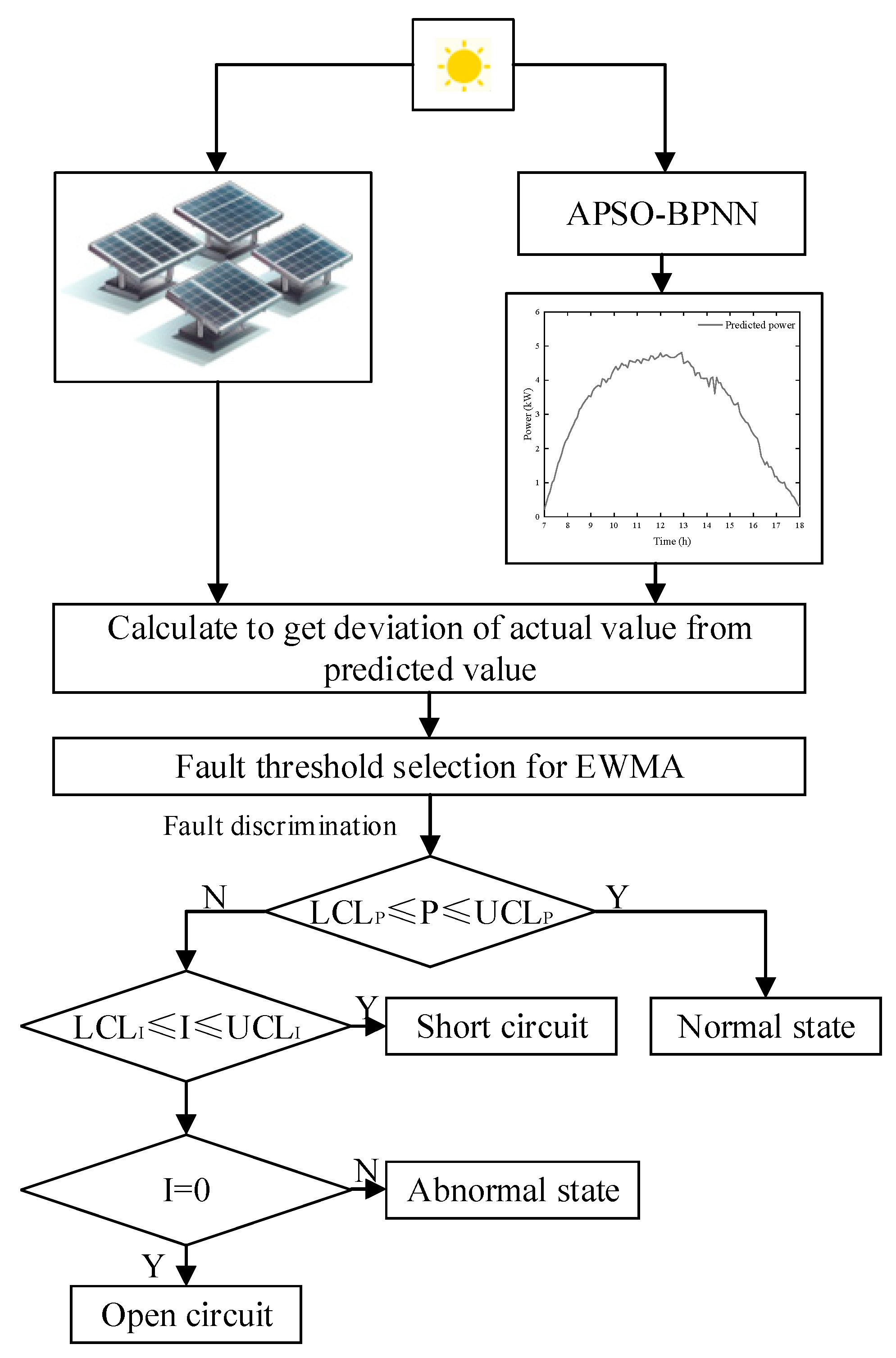
2.4. The Overall Model

Fault diagnosis is divided into two stages: PV power prediction and fault diagnosis based on the EWMA control chart. In the predictive model, the irradiance data are utilised as the input variable, with PV power generation as the output. Initially, an analysis of the solar power system’s historical performance data under comparable irradiance conditions is conducted, leading to the establishment of baseline performance metrics. These metrics are subsequently applied to train the model using future irradiance. By integrating the predicted irradiance with the established baseline performance, the anticipated PV power output is calculated. The historical data, together with prediction results, are employed as training and testing sets within the model, facilitating precise forecasting of future PV power generation. The following are the general steps of the suggested fault detection model, and its flowchart is shown in Figure 4.

• Obtain historical irradiance to analyse and establish baseline performance metrics;
• Train on irradiance to get predicted data and analyse them with baseline performance metrics to compare with actual irradiance;
• Obtain historical PV power data, clean the abnormal data, and normalise the data;
• Using APSO-BPNN, optimise the weights and thresholds of BPNN using APSO to get the PV predicted power;
• Calculate the variation between the actual power and the predicted power and select a fault diagnosis threshold for the EWMA chart;
• Simulate various fault types, analyse them using the method proposed, and compare them with the DR analysis method to verify the superiority of the EWMA method.

3. Case Study

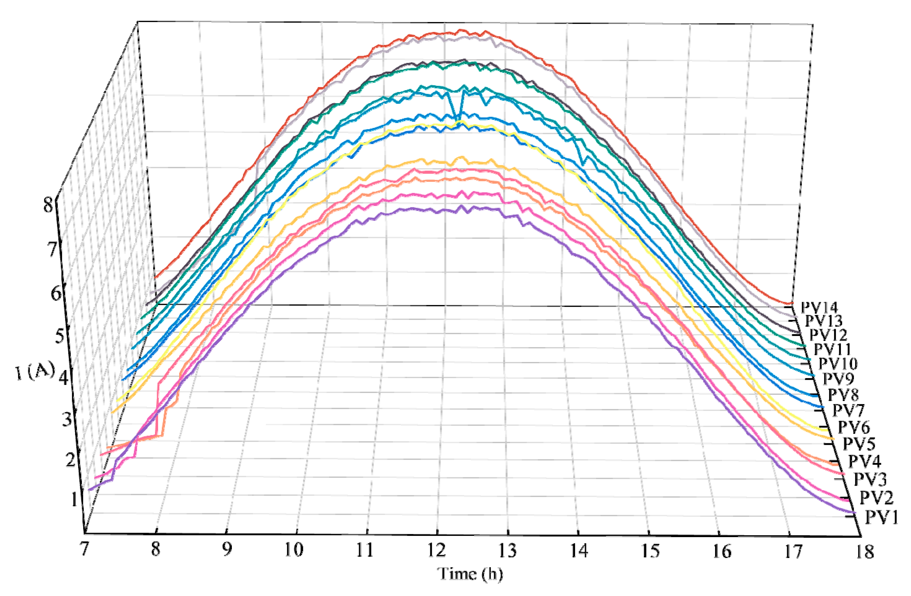
3.1. Data Description

The photovoltaic power data are sourced from one of the 110 KV inverters of a distributed 445.5 kWp PV power station located in Xiamen, Fujian, as depicted in Figure 5. The PV panels used in this station are 990 pieces of 450 W from LUXPOWER, and the inverter belongs to Huawei’s SUN2000 with a rating of 110 kW. The irradiance data are derived from the local meteorological station. In addition, it is also equipped with a cloud platform that continuously collects power generation data, meteorological data, and irradiance data using a thermoelectric total solar radiation sensor. The environmental monitoring interface is shown in Figure 6. The data were collected between 07:00 and 18:00 from February 27 to March 5, encompassing a total of 11 h with a sampling interval of 5 min. From the collected dataset, six days were selected to form the training set, while the remaining data were utilised as the test set.

Figure 7 illustrates the collected data for photovoltaic generation and irradiance curves across all strings in a single inverter under various meteorological conditions over a week. Particularly, the data for the second day show large fluctuations, which is due to the cloudy weather on that day. Clouds cause intermittent fluctuations in PV power generation when radiation intensity is high. Overall, the fluctuations in PV power generation are roughly in line with the fluctuations in radiation intensity.

Figure 8 presents the current curves for each string, demonstrating uniform variation across all strings.

3.2. Evaluation Metrics

The results of the prediction model were evaluated utilising the following three evaluation metrics: $R^2$, root mean square error (RMSE) and mean absolute error (MAE), whose expressions are shown in

Table 1. Evaluation metrics.

Metrics	Formula
$R^2$	$R^2=1-{\displaystyle \frac{{\displaystyle \sum _{\mathrm{i}}{(P_{pre}^i-P_{ture}^i)}^2}}{{\displaystyle \sum _{\mathrm{i}}{(P_{avg}^i-P_{ture}^i)}^2}}}$
RMSE	$RMSE=\sqrt{{\displaystyle \frac{1}{m}}{\displaystyle \sum _{i=1}^{\mathrm{m}}{(P_{pre}^i-P_{ture}^i)}^2}}$
MAE	$MAE={\displaystyle \frac{100\%}{m}}{\displaystyle \sum _{i=1}^{\mathrm{m}}\left|P_{pre}^i-P_{ture}^i\right|}$

$P_{pre}^i$, $P_{ture}^i$, and $P_{avg}^i$ are the predicted, actual, and average values, respectively.

below.

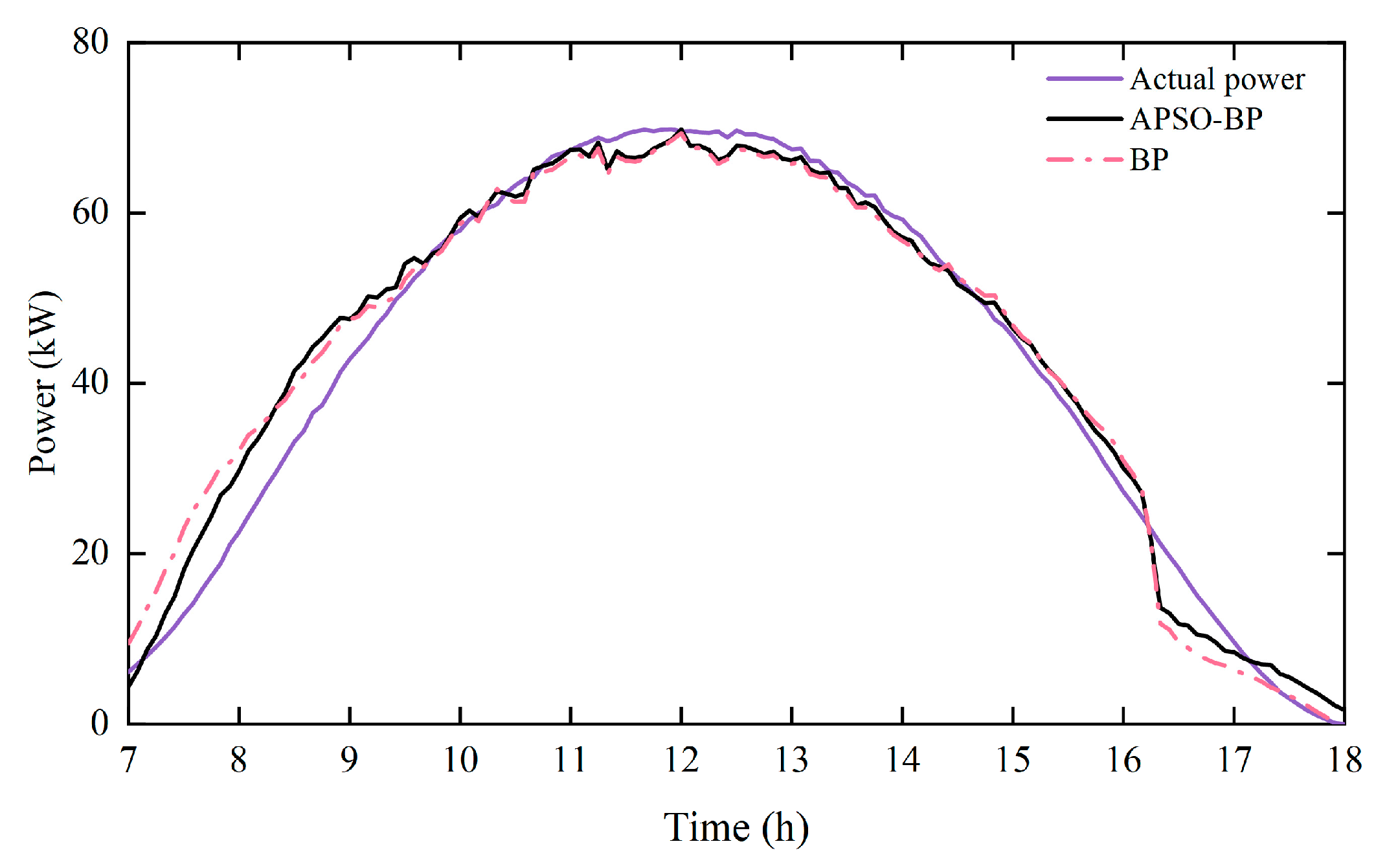
3.3. Analysis of Predicted Results

The methods proposed in this paper were implemented in MATLAB 2022b. In order to reduce the sensitivity of the prediction model to unusual values and enhance the model’s rate of convergence, the historical data were first cleaned and normalised. Then, the irradiance data were used as input for the APSO-BP model, while the current of each group of strings of the inverter was selected as the output value. The current prediction result was multiplied by the corresponding voltage value to obtain the predicted power of each group of strings. Then, the predicted power from all groups of strings was superimposed to obtain the final predicted power. The efficacy of this prediction model was further validated through a comparative analysis with the prediction results of the BPNN. The predicted results are shown in Figure 9 below.

As illustrated in Figure 9, compared with the BPNN model, the APSO-BP model showed higher prediction accuracy. The APSO effectively adapted the weights and thresholds of the BPNN during the optimisation process. Thus, the model can avoid falling into a locally optimal solution and achieve better global performance.

For the proposed model, the evaluation metrics are displayed in

Table 2. Predicted metrics results.

Model	${\mathit{R}}^2$	RMSE	MAE
APSO-BP	0.98	3.4	2.6
BP	0.96	4.3	3.2

below. Based on Table 1, it is evident that the APSO-BP model achieved a value of 0.98 for $R^2$, which shows an excellent fit and is superior to the traditional BPNN model. The closer the value of $R^2$ its value is to 1, it indicates that the model is capable of interpreting the data and predicting the results more accurately. Other evaluation metrics also suggest that the APSO-BP model appears to outperform the BPNN model. These indicators reflect the advantages of the APSO-BP model in terms of accuracy and stability.

4. Analysis of Photovoltaic Faults

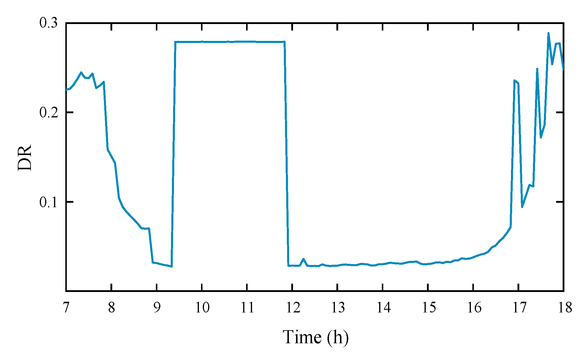
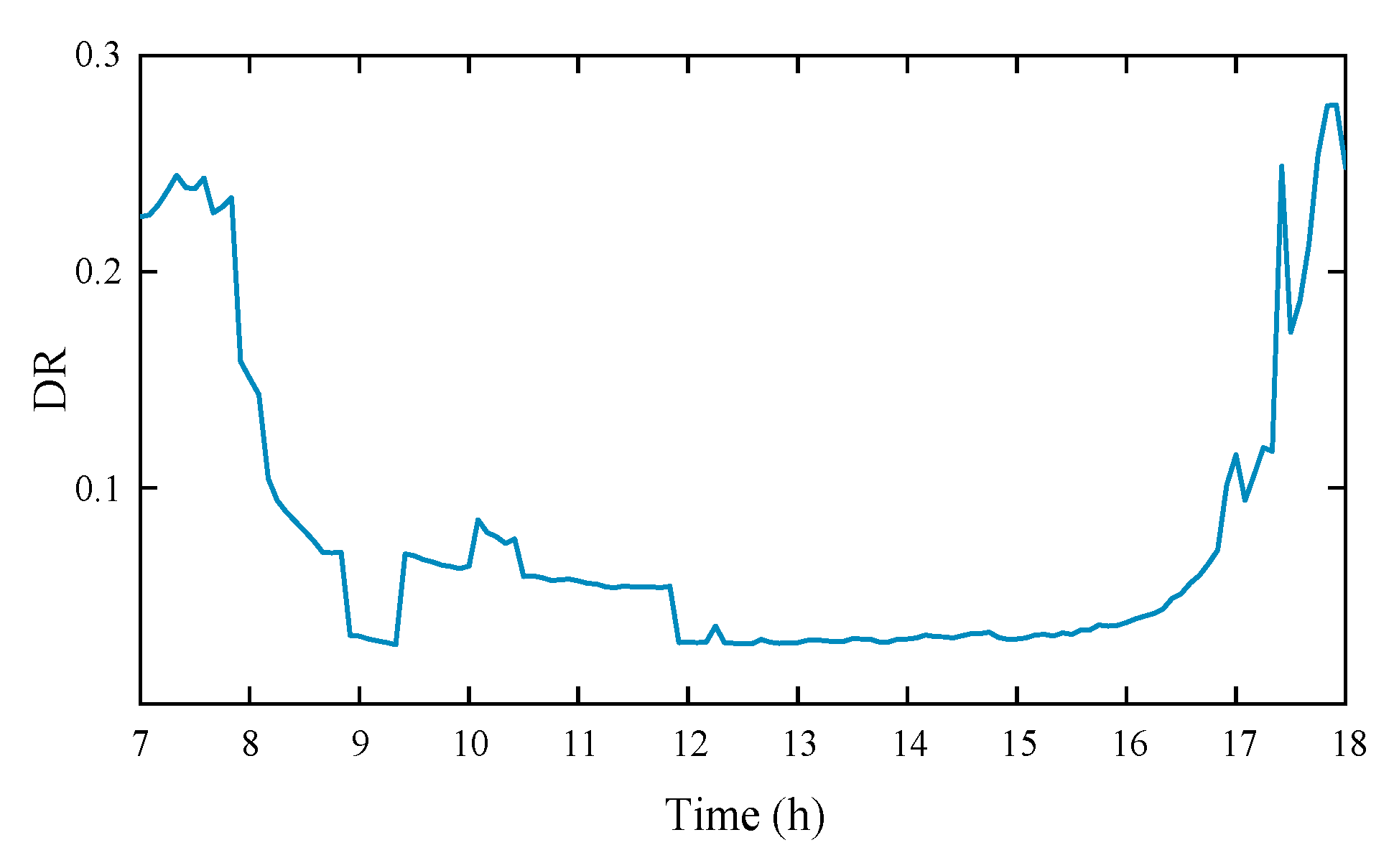
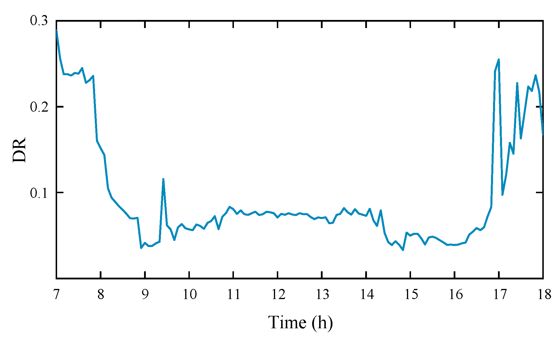
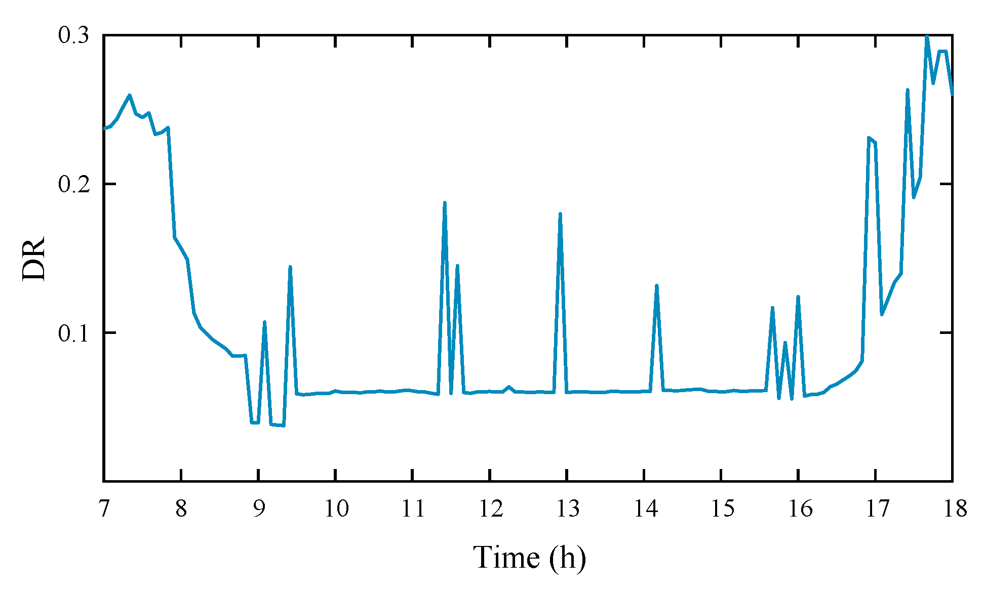
4.1. Photovoltaic Discrete Rate Analysis Method

In this case, the string power of this inverter is selected for analysis. The DR curves under normal conditions are represented in Figure 10.

The above-shown figure shows that the DR may be higher in the morning and evening due to the high variation of irradiation. At the same time, it should be lower at noon when the irradiation reaches its peak and is comparatively stable. The range of values of string dispersion mentioned in [35] is summarised in

Table 3. Range of values for the discrete rate of string current.

Range of Values	State
0–0.05	Stable
0.05–0.1	Favourable
0.1–0.2	Need to improve
>0.2	Poor

.

4.1.1. Open Circuit

In this case, the DC cable wiring of the PV array is disconnected to simulate the open circuit. Figure 11 displays the DR curve.

In the event of an open circuit fault, certain strings no longer produce current, and the power output of that section drops significantly to zero, resulting in a decrease in the mean value of the overall power output and an increase in the standard deviation. Consequently, the DR rises significantly. In excellent lighting conditions, the DR curve spikes, and the fault effect is even more pronounced.

4.1.2. Short Circuit

By shorting the PV modules, a short circuit defect can be emulated. The DR curve is shown in Figure 12 below. A short circuit causes a decrease in power production for part of the time, which can lead to an increase in the standard deviation of the output, showing sudden peaks that may be followed by a rapid drop due to the intervention of system protection actions.

4.1.3. Abnormal State

Both glass breakage and dust shading in PV modules result in diminished solar irradiance reception, thereby reducing the efficiency of power generation. The DR curves are shown in Figure 13 and Figure 14 below. During abnormal conditions, the power outputs become unstable, and these variations are usually more persistent than open and short circuit faults.

4.1.4. DC Side Ground Fault

In this case, it is noticed that the PV ground fault is induced by the poor contact of the multi-contact 4 (MC4) plug. When poor contact occurs at the MC4 interface, an elevated resistance is formed at the connection point, which increases the resistance to the current passage. This high resistance at the contact point may generate overheating due to the current passage, and this overheating may indirectly lead to ground faults. The DR curves are shown in Figure 15.

After the DR stabilises below 0.05, significant fluctuations begin to occur, indicating a system failure. A DC side ground fault causes the voltage to plummet and the current to become unstable, which leads to a sudden drop in power and an increase in the DR.

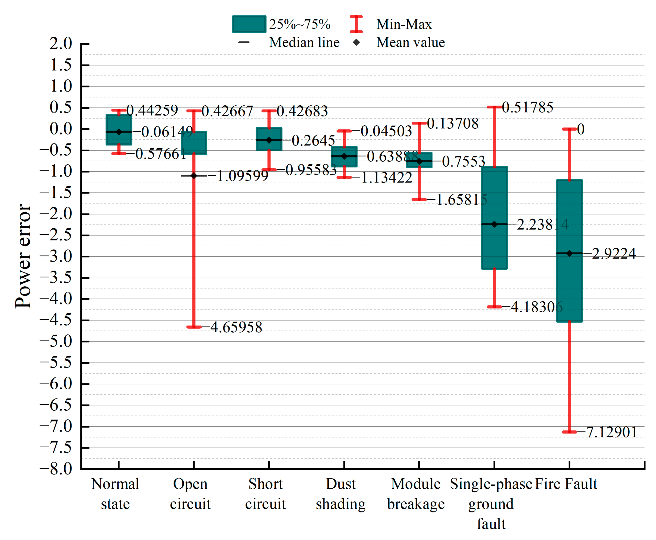
4.2. Fault Diagnosis Method Based on EWMA Control Chart

In this study, an EWMA chart was utilised to detect faults in the PV system by monitoring the error between predicted and actual values. This method detects potential fault situations by tracking future error changes. To ascertain the effectiveness of this method, it was also analysed for the same fault situations.

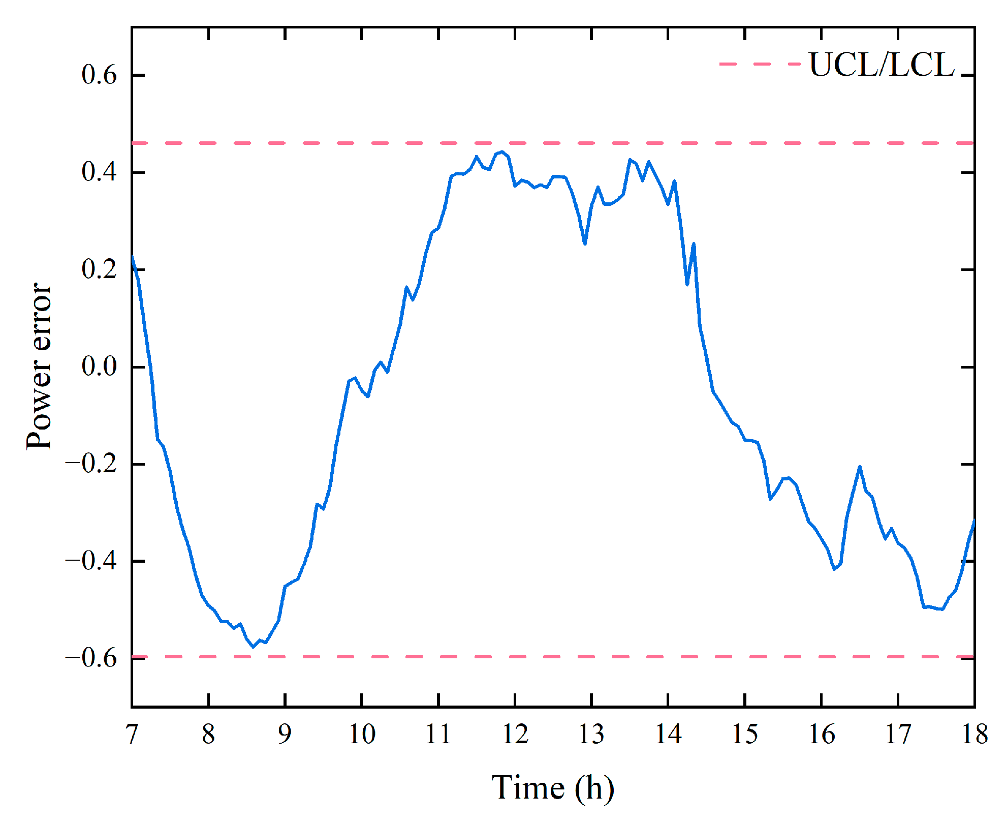
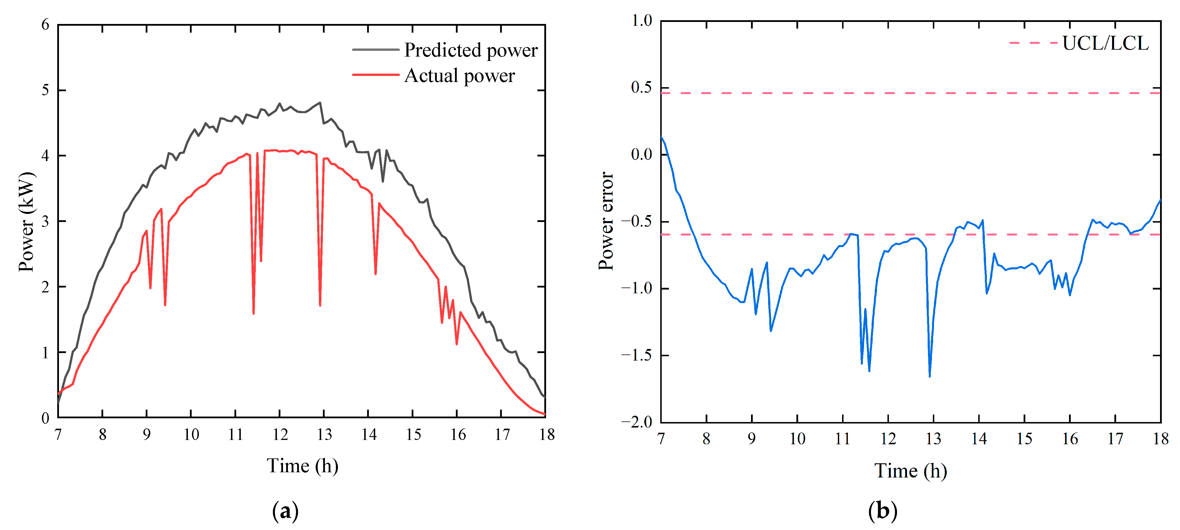
4.2.1. Normal State

Under normal conditions, the power EWMA control chart is shown in Figure 16. It is observed that this control quantity always falls within the range of the upper and lower control limits, indicating that the PV array is generating power typically, and illustrating the accurate description of the PV non-fault state by the EWMA chart.

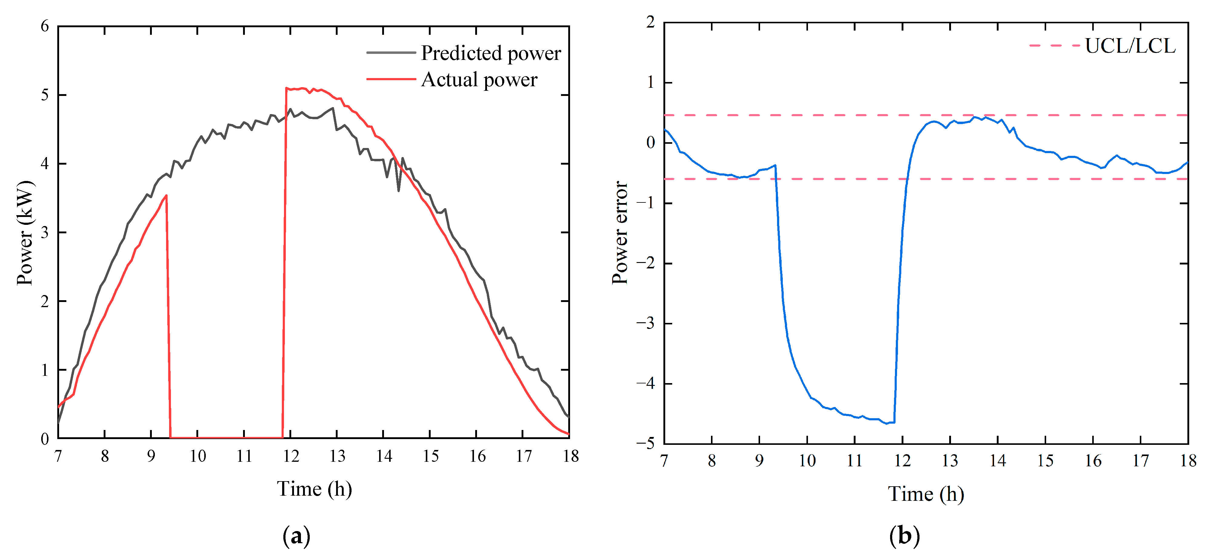
4.2.2. Open Circuit

Figure 17a illustrates the power curve during an open-circuit fault, where the PV power drops abruptly to zero due to the disconnection of the current. The corresponding EWMA control chart (Figure 17b) shows that during an open-circuit fault, the controlled quantity is significantly lower than the control limit. This sudden drop clearly indicates the presence of an open-circuit fault within the PV string.

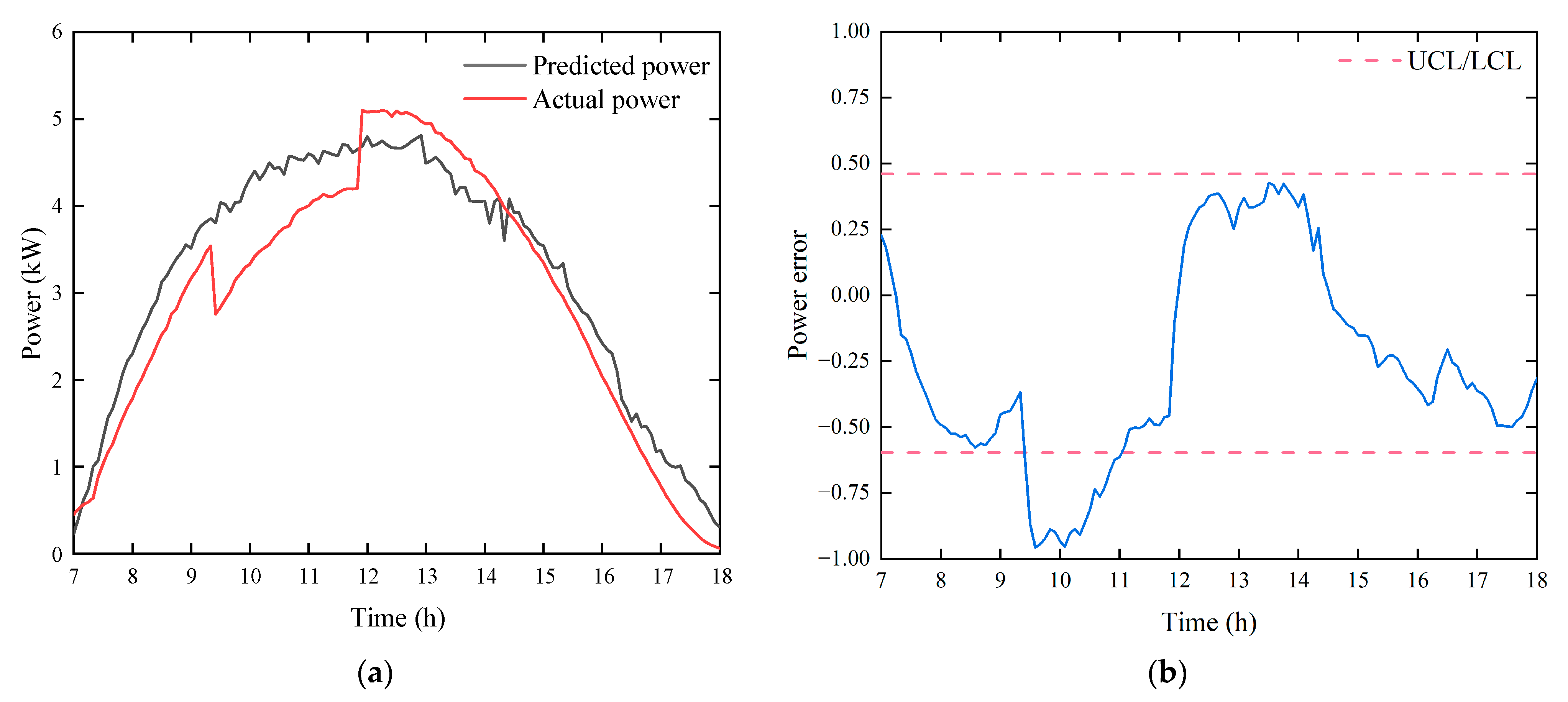
4.2.3. Short Circuit

The power curve at the occurrence of the short-circuit fault is illustrated in Figure 18a, showing a significant loss of power, followed by a return to normal after fault recovery. The EWMA chart in Figure 18b similarly indicates that during the fault, the control quantity falls below the lower control limit, effectively pointing to an abnormal state.

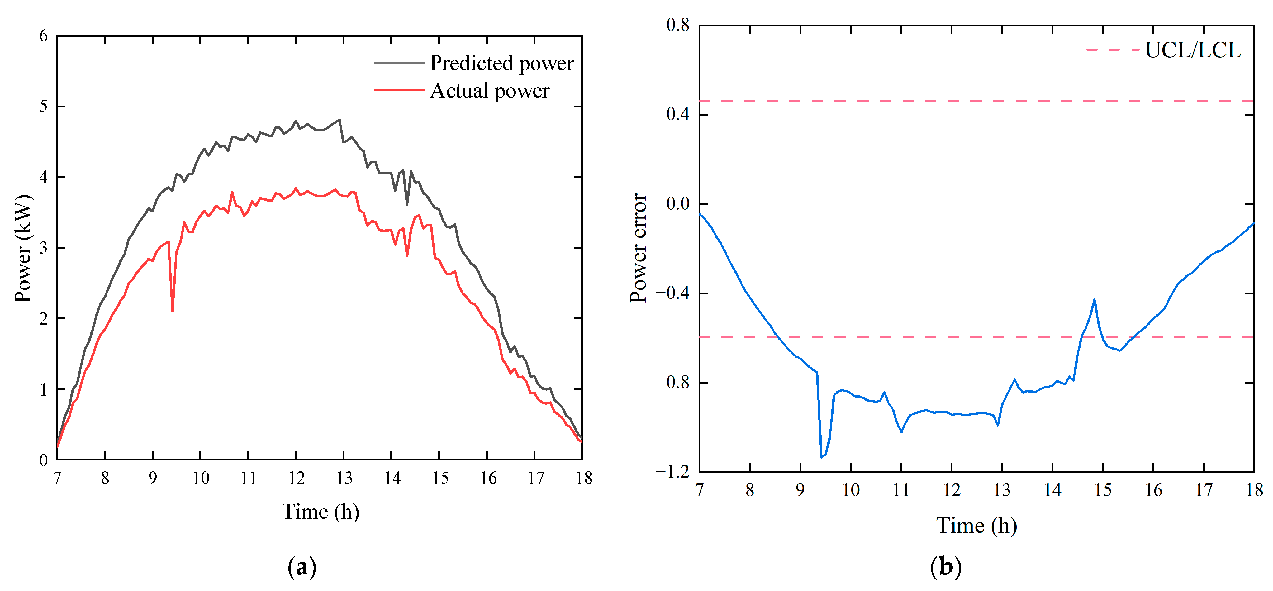
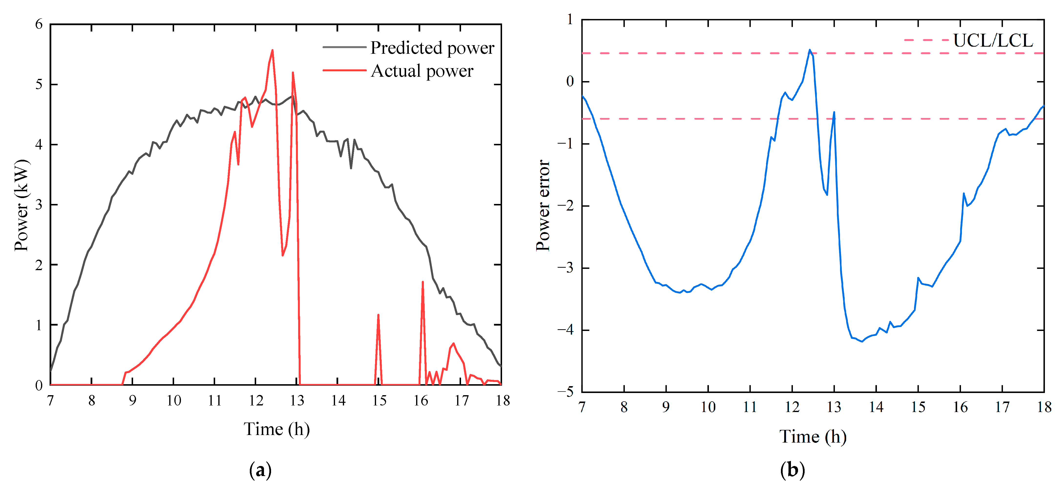
4.2.4. Abnormal State

Although open-circuit and short-circuit faults are more obvious and easily detected, there are many abnormal states in the system, which are difficult to be detected at an early stage by traditional methods. Through the efficient learning and adaptive capability of neural networks, potential hidden faults in the system can be detected and predicted in time to improve the accuracy and efficiency, thus ensuring the stability and reliability of the system. The power curves in Figure 19a and Figure 20a demonstrate the effect of dust shading and module breakage on the conversion efficiency of the PV module, resulting in a consistently lower output power than predicted.

The EWMA charts (Figure 19b and Figure 20b) show that the control quantities consistently lie outside the control limits, clearly indicating the occurrence of a fault. This analysis demonstrates that the EWMA chart is an effective tool for monitoring performance degradation due to dust accumulation or physical damage.

4.2.5. DC Side Ground Fault

The fault curves are shown in Figure 20. What can be seen in the EWMA chart according to Figure 21b is the typical behavior of this fault in a PV module. The power error started to decrease rapidly from close to zero, which can be attributed to the initial phase of the DC side ground fault resulting in partial loss of power. At around 13:00, the power shown in Figure 21a plummeted to zero, at which point the power error reached its lowest point, which is significantly below the lower control limit, indicating that the system was severely affected during this time period. This dramatic fluctuation may be related to the effects of irradiation and temperature on ground faults.

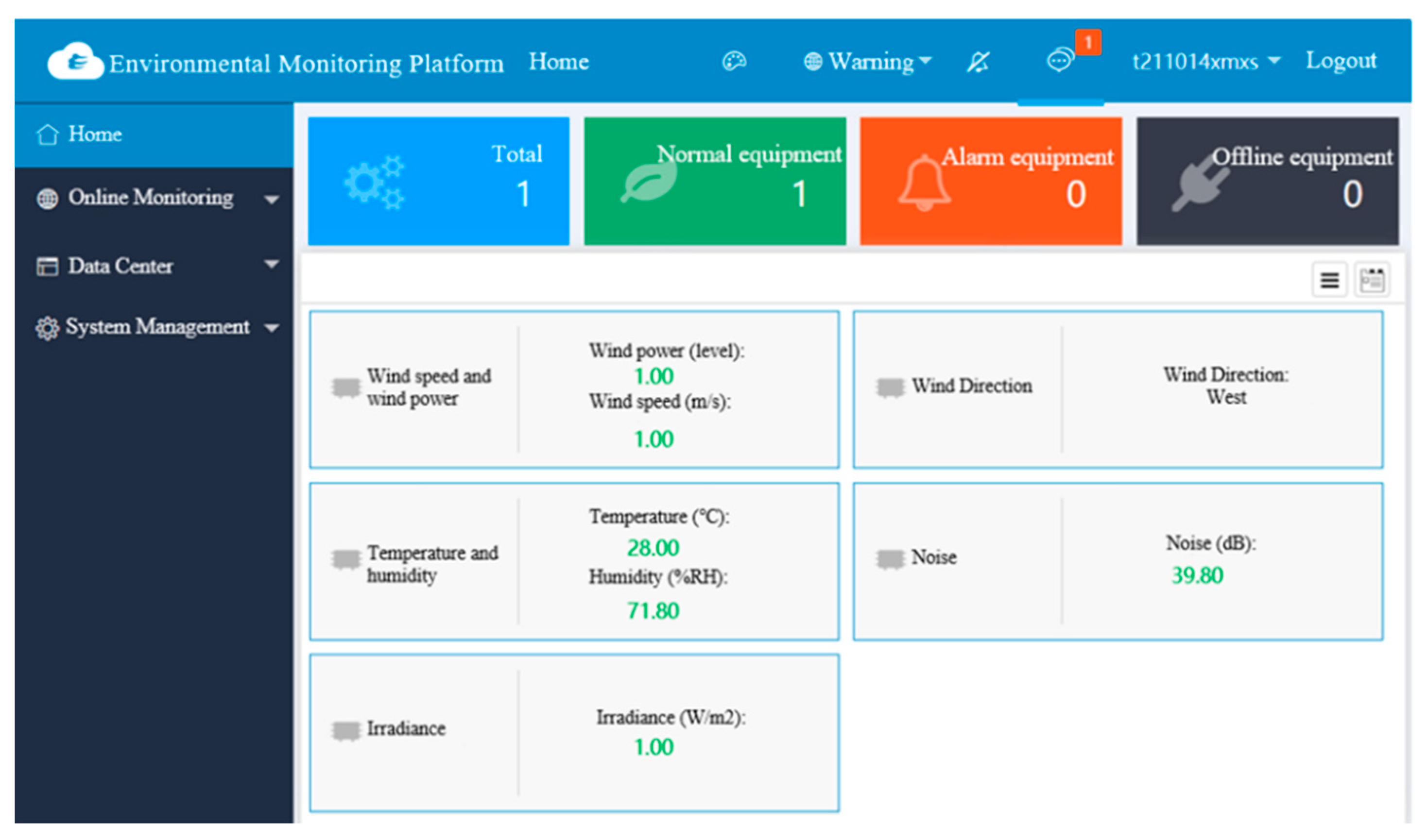
4.3. Realistic Scenario

In this study, critical parameters including irradiance, temperature, and humidity serve as inputs to the APSO-BP model for predicting the anticipated power output of the photovoltaic system under fault-free conditions. The outcomes of these predictions are depicted in Figure 22a. A comparison between the model’s predicted power output and the actual power output reveals a substantial discrepancy.

This discrepancy implies that various unforeseen factors might compromise the performance of the PV system. These could encompass ageing equipment, inadequate maintenance, or abrupt environmental alterations. Notably, in extreme conditions such as fires, the power output of PV panels could be considerably diminished owing to structural damage or obstructions caused by coverings.

A collection of fault current data preceding and subsequent to the fault event was meticulously selected and subjected to rigorous analysis utilising the EWMA control chart. As illustrated in Figure 22b, the distinctly marked points 1 and 2 notably surpassed the established upper and lower thresholds of the control chart. This error implies a potential malfunction within the system. It is noted that the current value demonstrated multiple pronounced fluctuations within a markedly brief interval. These fluctuations comprise both rapid escalations and declines in current, as well as periods where the current intermittently reverts to zero. This erratic current performance is particularly prominent on the EWMA control chart, resulting in frequent up-and-down fluctuations on the EWMA control chart. Specifically, these fluctuations are not only frequent but intense enough to cause the EWMA value to exceed the set upper and lower control limits. Such breaches serve as crucial warning indicators within a monitoring framework, suggesting the potential existence of a substantial technical issue within the current control system. The observed pattern of fluctuations bears a striking resemblance to the characteristics typically associated with a DC-side ground fault. Given these observations, it can be inferred with a reasonable degree of certainty that a DC side ground fault likely occurred within this inverter system. Consequently, appropriate maintenance interventions are necessitated to rectify the issue.

The analysis of the above-shown EWMA charts can be summarised as a box plot, as shown in Figure 23.

Analysis of this box plot clearly delineates the impact of various fault types on the performance of the PV system. Under the normal state, the system exhibited stable performance with minimal errors, while open circuit and DC side ground faults led to substantial power degradation characterised by significant errors. Short circuits, module breakage, and dust shading affected the PV power efficiency, but the impact was mild.

Through these analyses, it is apparent that while traditional DR analysis can evaluate the overall performance of the inverter and detect faults, it frequently lacks the precision to identify the specific location of these faults. In contrast, the EWMA control chart overcomes this limitation. By monitoring errors between predicted and actual power outputs, this method not only promptly detects anomalies within the inverter but also accurately identifies the specific string experiencing the fault. This facilitates rapid diagnostic and maintenance decisions, thereby enhancing the accuracy of fault diagnosis and optimising the maintenance and operational efficiency of the system.

5. Conclusions

In the daily O&M of PV systems, it is particularly essential to have a stable operation of the power plant due to its long-term exposure to complex and changing environmental conditions, which are influenced by various factors. To enhance the efficiency of fault identification, this work presents a fault diagnosis strategy that integrates the PV power prediction model and the EWMA control chart. The strategy adopts the APSO-BPNN model to predict PV power with high accuracy. Subsequently, the types of faults, such as open and short circuits that may occur in the PV system, were analysed in detail using DR analysis and the EWMA control chart.

The results revealed that the APSO-BPNN model had excellent performance in PV power prediction, with the $R^2$ metric as high as 0.98, which verifies the high prediction accuracy of the model. Meanwhile, compared with the traditional DR analysis method, the EWMA control chart showed higher accuracy in fault localisation, capable of effectively identifying and locating specific fault strings. Therefore, the fault diagnosis method integrating the APSO-BPNN model and the EWMA control chart provides a more efficient and precise solution for the O&M management of PV power plants. This method substantially enhances O&M response times and power generation efficiency, thus holding significant importance for promoting the sustainable development of the PV industry. In addition, this method is an advanced data-driven approach that has the advantage of not requiring complex physical modelling of the PV plant. It is not required to factor in the effects of variables such as cable length and the excessive number of modules on the model. Given the extensive size of the PV plant operation database, which facilitates the construction and utilisation of persistent models, along with a comprehensive consideration of the reliability of diagnostic methods and the practicality of engineering applications, the use of more complex machine learning models is deemed inappropriate.

Moreover, given the inherent similarities and complementarities among renewable energy systems, it is anticipated that the synergistic integration of the APSO-BPNN model with the EWMA control chart will be equally efficacious in wind and hydroelectric systems. Within these contexts, the APSO-BPNN model is poised to enhance the accuracy of predictions concerning critical variables such as wind speed and water flow. Concurrently, the EWMA control chart is capable of meticulously monitoring equipment performance, enabling the prompt identification and localisation of systemic anomalies. By broadening the scope of this application to encompass these domains, it is projected that not only will the efficiency of energy capture be augmented, but operational and maintenance costs will also be substantially diminished, thereby fostering both technological progression and economic sustainability within the broader renewable energy sector.

Although the method proposed in the paper performs well in PV plant fault diagnosis, it still needs to face challenges such as computational complexity and data processing. Future work can further improve the algorithm to increase the prediction speed and accuracy of the model. Meanwhile, the value of the smoothing coefficient can be optimised in the EWMA chart to find a more suitable control interval.

References

- Huang, S.; Zhou, Q.; Shen, J.; Zhou, H.; Yong, B. Multistage Spatio-Temporal Attention Network Based on NODE for Short-Term PV Power Forecasting. Energy 2024, 290, 130308. [Google Scholar] [CrossRef]
- Balachandran, G.B.; Devisridhivyadharshini, M.; Ramachandran, M.E.; Santhiya, R. Comparative Investigation of Imaging Techniques, Preprocessing and Visual Fault Diagnosis Using Artificial Intelligence Models for Solar Photovoltaic System–A Comprehensive Review. Measurement 2024, 232, 114683. [Google Scholar] [CrossRef]
- Guo, H.; Hu, S.; Wang, F.; Zhang, L. A Novel Method for Quantitative Fault Diagnosis of Photovoltaic Systems Based on Data-Driven. Electr. Power Syst. Res. 2022, 210, 108121. [Google Scholar] [CrossRef]
- Alam, M.K.; Khan, F.; Johnson, J.; Flicker, J. A Comprehensive Review of Catastrophic Faults in PV Arrays: Types, Detection, and Mitigation Techniques. IEEE J. Photovolt. 2015, 5, 982–997. [Google Scholar] [CrossRef]
- Hong, Y.-Y.; Pula, R.A. Methods of Photovoltaic Fault Detection and Classification: A Review. Energy Rep. 2022, 8, 5898–5929. [Google Scholar] [CrossRef]
- Ding, K.; Chen, X.; Jiang, M.; Yang, H.; Chen, X.; Zhang, J.; Gao, R.; Cui, L. Feature Extraction and Fault Diagnosis of Photovoltaic Array Based on Current–Voltage Conversion. Appl. Energy 2024, 353, 122135. [Google Scholar] [CrossRef]
- Zhang, C.; Peng, T.; Nazir, M.S. A Novel Integrated Photovoltaic Power Forecasting Model Based on Variational Mode Decomposition and CNN-BiGRU Considering Meteorological Variables. Electr. Power Syst. Res. 2022, 213, 108796. [Google Scholar] [CrossRef]
- Qi, X.; Chen, Q.; Zhang, J. Short-Term Prediction of PV Power Based on Fusions of Power Series and Ramp Series. Electr. Power Syst. Res. 2023, 222, 109499. [Google Scholar] [CrossRef]
- Harrou, F.; Sun, Y.; Taghezouit, B.; Saidi, A.; Hamlati, M.-E. Reliable Fault Detection and Diagnosis of Photovoltaic Systems Based on Statistical Monitoring Approaches. Renew. Energy 2018, 116, 22–37. [Google Scholar] [CrossRef]
- Wang, L.; Mao, M.; Xie, J.; Liao, Z.; Zhang, H.; Li, H. Accurate Solar PV Power Prediction Interval Method Based on Frequency-Domain Decomposition and LSTM Model. Energy 2023, 262, 125592. [Google Scholar] [CrossRef]
- Meenal, R.; Selvakumar, A.I. Assessment of SVM, Empirical and ANN Based Solar Radiation Prediction Models with Most Influencing Input Parameters. Renew. Energy 2018, 121, 324–343. [Google Scholar] [CrossRef]
- Pedro, H.T.C.; Coimbra, C.F.M. Assessment of Forecasting Techniques for Solar Power Production with No Exogenous Inputs. Sol. Energy 2012, 86, 2017–2028. [Google Scholar] [CrossRef]
- Li, P.; Zhou, K.; Lu, X.; Yang, S. A Hybrid Deep Learning Model for Short-Term PV Power Forecasting. Appl. Energy 2020, 259, 114216. [Google Scholar] [CrossRef]
- Tian, W.; Bao, Y.; Liu, W. Wind Power Forecasting by the BP Neural Network with the Support of Machine Learning. Math. Probl. Eng. 2022, 2022, 7952860. [Google Scholar] [CrossRef]
- Zhao, Y.; Li, D.; Lu, T.; Lv, Q.; Gu, N.; Shang, L. Collaborative Fault Detection for Large-Scale Photovoltaic Systems. IEEE Trans. Sustain. Energy 2020, 11, 2745–2754. [Google Scholar] [CrossRef]
- Jiang, M.; Ding, K.; Chen, X.; Cui, L.; Zhang, J.; Yang, Z.; Cang, Y.; Cao, S. Research on Time-Series Based and Similarity Search Based Methods for PV Power Prediction. Energy Convers. Manag. 2024, 308, 118391. [Google Scholar] [CrossRef]
- Saxena, N.; Kumar, R.; Rao, Y.K.; Mondloe, D.S.; Dhapekar, N.K.; Sharma, A.; Yadav, A.S. Hybrid KNN-SVM Machine Learning Approach for Solar Power Forecasting. Environ. Chall. 2024, 14, 100838. [Google Scholar] [CrossRef]
- Yuan, Z.; Xiong, G.; Fu, X. Artificial Neural Network for Fault Diagnosis of Solar Photovoltaic Systems: A Survey. Energies 2022, 15, 8693. [Google Scholar] [CrossRef]
- Alsafasfeh, M.; Abdel-Qader, I.; Bazuin, B.; Alsafasfeh, Q.; Su, W. Unsupervised Fault Detection and Analysis for Large Photovoltaic Systems Using Drones and Machine Vision. Energies 2018, 11, 2252. [Google Scholar] [CrossRef]
- Li, Y.; Ding, K.; Zhang, J.; Chen, F.; Chen, X.; Wu, J. A Fault Diagnosis Method for Photovoltaic Arrays Based on Fault Parameters Identification. Renew. Energy 2019, 143, 52–63. [Google Scholar] [CrossRef]
- Shin, J.-H.; Kim, J.-O. On-Line Diagnosis and Fault State Classification Method of Photovoltaic Plant. Energies 2020, 13, 4584. [Google Scholar] [CrossRef]
- Lu, X.; Lin, P.; Cheng, S.; Lin, Y.; Chen, Z.; Wu, L.; Zheng, Q. Fault Diagnosis for Photovoltaic Array Based on Convolutional Neural Network and Electrical Time Series Graph. Energy Convers. Manag. 2019, 196, 950–965. [Google Scholar] [CrossRef]
- Chine, W.; Mellit, A.; Lughi, V.; Malek, A.; Sulligoi, G.; Pavan, A.M. A Novel Fault Diagnosis Technique for Photovoltaic Systems Based on Artificial Neural Networks. Renew. Energy 2016, 90, 501–512. [Google Scholar] [CrossRef]
- Junjie, W.; Dedong, G.; Shaokang, Z.; Shan, W.; Haixiong, L. Fault Diagnosis Method of Photovoltaic Array Based on Support Vector Machine. Energy Sources Part A Recovery Util. Environ. Eff. 2019, 45, 5380–5395. [Google Scholar] [CrossRef]
- Huang, J.-M.; Wai, R.-J.; Yang, G.-J. Design of Hybrid Artificial Bee Colony Algorithm and Semi-Supervised Extreme Learning Machine for PV Fault Diagnoses by Considering Dust Impact. IEEE Trans. Power Electron. 2019, 35, 7086–7099. [Google Scholar] [CrossRef]
- Kennedy, J.; Eberhart, R. Particle Swarm Optimization. In Proceedings of the ICNN’95-International Conference on Neural Networks, Perth, Australia, 27 November–1 December 1995; Volume 4, pp. 1942–1948. [Google Scholar]
- Huang, W.; Liu, H.; Zhang, Y.; Mi, R.; Tong, C.; Xiao, W.; Shuai, B. Railway Dangerous Goods Transportation System Risk Identification: Comparisons among SVM, PSO-SVM, GA-SVM and GS-SVM. Appl. Soft Comput. 2021, 109, 107541. [Google Scholar] [CrossRef]
- Moayedi, H.; Mehrabi, M.; Mosallanezhad, M.; Rashid, A.S.A.; Pradhan, B. Modification of Landslide Susceptibility Mapping Using Optimised PSO-ANN Technique. Eng. Comput. 2019, 35, 967–984. [Google Scholar] [CrossRef]
- Yang, D.-W.; Li, H.-R.; Xiang, W.-D.; Ren, Z.; Li, Z.-W. Power Transformer Fault Diagnosis Based on Improved PSO-BP Hybrid Algorithm. J. Electr. Power Sci. Technol. 2011, 26, 99–103. [Google Scholar] [CrossRef]
- Zhang, Y.; Cui, N.; Feng, Y.; Gong, D.; Hu, X. Comparison of BP, PSO-BP and Statistical Models for Predicting Daily Global Solar Radiation in Arid Northwest China. Comput. Electron. Agric. 2019, 164, 104905. [Google Scholar] [CrossRef]
- Li, Y.; Huang, W.; Lou, K.; Zhang, X.; Wan, Q. Short-Term PV Power Prediction Based on Meteorological Similarity Days and SSA-BiLSTM. Syst. Soft Comput. 2024, 6, 200084. [Google Scholar] [CrossRef]
- Liang, W.; Mukherjee, A.; Xiang, D.; Xu, Z. A New Nonparametric Adaptive EWMA Procedures for Monitoring Location and Scale Shifts via Weighted Cucconi Statistic. Comput. Ind. Eng. 2022, 170, 108321. [Google Scholar] [CrossRef]
- Mishra, A.K.; Das, B. A Scheme for Electricity Theft Detection Based on EWMA Control Chart. Electr. Power Syst. Res. 2024, 230, 110277. [Google Scholar] [CrossRef]
- Garoudja, E.; Harrou, F.; Sun, Y.; Kara, K.; Chouder, A.; Silvestre, S. Statistical Fault Detection in Photovoltaic Systems. Sol. Energy 2017, 150, 485–499. [Google Scholar] [CrossRef]
- Fu, G.; Li, X.; Gao, X. Analytical Method and Application of Current Discrete Rate of PV Power Station Based on Junction Box String. Power Syst. Clean Energy 2014, 30, 109–113. [Google Scholar] [CrossRef]