Precision Control for Room Temperature of Variable Air Volume Air-Conditioning Systems with Large Input Delay

Abstract

A large input delay, parametric uncertainties, matched disturbances and mismatched disturbances exist extensively in variable air volume air-conditioning systems, which can deteriorate the control performance of the room temperature and even destabilize the system. To address this problem, an adaptive-gain command filter control framework for the room temperature of variable air volume air-conditioning systems is exploited. Through skillfully designing an auxiliary system, both the filtered error and the input delay can be compensated concurrently, which can attenuate the effect of the filtered error and the input delay on the control performance of the room temperature. Then, a smooth nonlinear term with an adjusted gain is introduced into the control framework to compensate for parametric uncertainties, matched disturbances and mismatched disturbances, which relieves the conservatism of the controller gain selection. With the help of the Lyapunov theory, both the boundedness of all the system signals and the asymptotic tracking performance for the room temperature can be assured with the presented controller. Finally, the contrastive simulation results demonstrate the validity of the developed method.

1. Introduction

Precision temperature control plays a key role in the reliability and service life of the precision electronic systems of critical infrastructure such as hospitals, data centers, operation control centers, chemical workshops and pharmaceutical workshops, which have strict requirements for temperature. As the core device for regulating room temperature, the variable air volume air-conditioning system (VAVACS) is widely applied in all kinds of constructions owing to its good energy saving and flexible control [1,2,3,4,5,6,7]. Nevertheless, due to the extensive existence of large input delay, parametric uncertainties, matched disturbances and mismatched disturbances in VAVACS, which makes it difficult for the room temperature to achieve the ideal control effect, the achievement of the expected control performance of the room temperature for VAVACS is challenging. To overcome this problem and gain an improvement in the control performance of the room temperature for VAVACS, a lot of control results have been exploited in the past few years.

Typically, proportional–integral–differential (PID)-based control frameworks are broadly employed in the control design of room temperature for VAVACS due to their simple structure and easy parameter tuning [8,9,10,11,12]. By uniting fuzzy PID and dynamic programming, Xie et al. developed an eco-cooling controller method with two layers for electric car air-conditioning systems [9], where fruitful experimental results have shown the validity of this approach. In [11], Li et al. presented a fractional-order PID control result for indoor temperature in an air-conditioning room, in which a modified ant colony optimization algorithm was utilized to further obtain the enhancement of control performance for the room temperature. However, the existence of a large input delay, parametric uncertainties, matched disturbances and mismatched disturbances in VAVACS, which can deteriorate the control performance of the room temperature and even destabilize the system, was not considered in the above-mentioned PID-based control approaches [8,9,10,11,12]. As a result, some model feedforward compensation-based control methods have been developed to further gain an improvement in the control performance of room temperature for VAVACS. In [13], a model-based optimal controller framework was presented for multizone VAVACS, in which the room pressure was neutralized, and the fan energy consumption could be reduced. In [14], an observer-based control framework was proposed to achieve the improvement of control performance. Also, Rsetam et al. designed a finite-time disturbance observer-based control scheme for air-conditioning systems in [15], where the finite-time disturbance observer was adopted to estimate the unknown disturbances and then achieve the active disturbance compensation in a finite amount of time, whereas the input delay of the systems was not taken into consideration in the above control methods.

The input delay can worsen the temperature control performance and make the VAVACS unstable. To weaken the impact of the input delay on the control performance, a predictor-based controller framework was developed in [16,17,18] to dispose of the input delay and matched disturbances, in which the controller stability could be ensured using the Lyapunov–Krasovskii theory. Also, the Pade approximation approach was applied in the controller design to ensure the achievement of adaptive tracking control for nonlinear input-delayed systems with mismatched disturbances in [19,20]. Ma et al. skillfully constructed an auxiliary system to remove the impact of time-variant input delay on the control performance in [21,22]. Subsequently, inspired by [21,22], the auxiliary system that can compensate for the time-varying input delay was extended to the adaptive filtered control results in [23,24]. Nonetheless, all the aforementioned control results in [16,17,18,19,20,21,22,23,24] could gain the bounded control performance in the presence of time-varying disturbances. Therefore, how to construct an asymptotic temperature control method for VAVACS with a large input delay, matched disturbances and mismatched disturbances is a challenging problem.

In this study, an adaptive-gain command filter control framework for room temperature of VAVACS was exploited. Through skillfully designing an auxiliary system, both the filtered error and the input delay can be compensated concurrently. Then, a smooth nonlinear term with an adjusted gain is introduced into the control framework to compensate for parametric uncertainties, matched disturbances and mismatched disturbances, which relieves the conservatism of the controller gain selection. Based on Lyapunov theory, both the boundedness of all the system signals and the asymptotic tracking performance for the room temperature can be assured with the presented controller. In the end, the contrastive simulation results demonstrate the validity of the developed method. The main contributions of this paper include the following. (1) An adaptive-gain command filter control framework is presented for the room temperature of variable air volume air-conditioning systems with a large input delay, matched disturbances and mismatched disturbances, where both the boundedness of all the system signals and the asymptotic tracking performance for the room temperature can be assured. (2) Through skillfully designing an auxiliary system, both the filtered error and the input delay can be compensated concurrently, which can attenuate the effect of the filtered error and the input delay on the control performance of the room temperature. (3) Through utilizing a smooth nonlinear term with an adjusted gain, the conservatism of the controller gain selection can be relaxed a lot.

The structure of this paper is as follows: Section 2 completes the modeling of the room temperature control of variable air volume air-conditioning systems. The controller design and its stability analysis can be found in Section 3. The simulation results and conclusions are presented in Section 4 and Section 5.

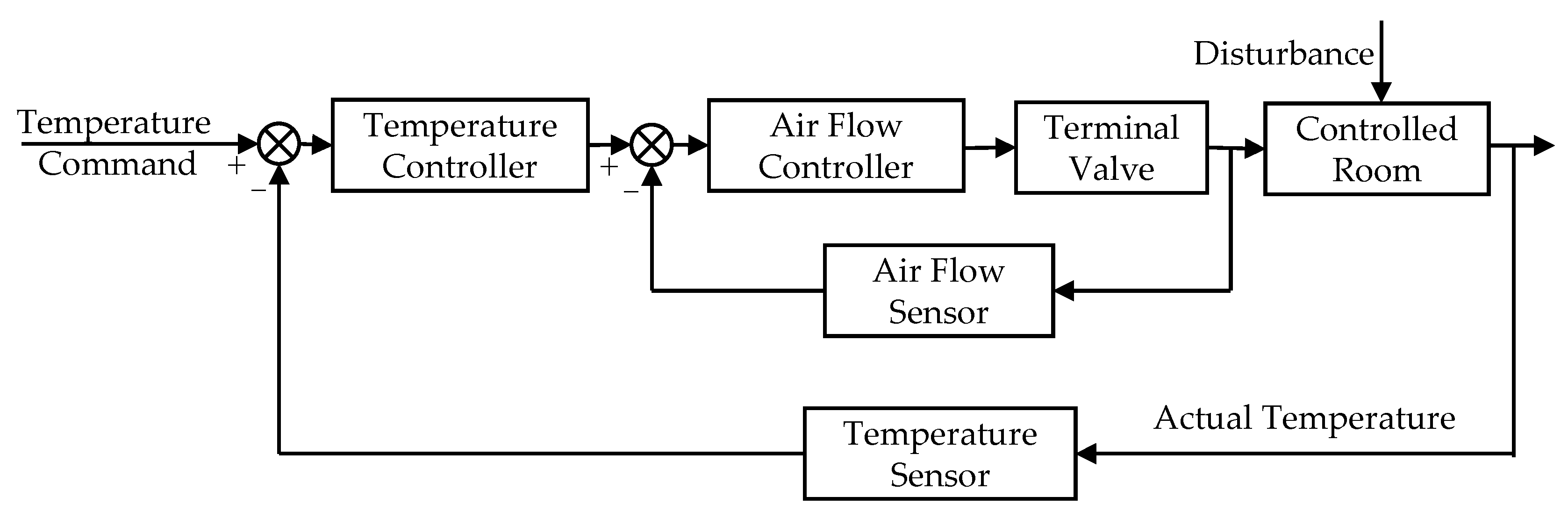
2. System Modeling

The studied principle of temperature control for a variable air volume air-conditioning system (VAVACS) is presented in Figure 1, where the terminal valve is employed to change the supplied air flow of the VAVACS such that the room temperature can be adjusted for demand.

According to the energy conservation equation, the thermodynamic model of the controlled room can be expressed by

$$c_r{\dot{T}}_n=Q_r+c\rho (T_s-T_n)Q_a+f_1(t)$$

(1)

in which $T_n$ denotes the indoor temperature; $T_s$ denotes the supply air temperature; c denotes the specific heat capacity of the air; $\rho$ denotes the density of the air; $Q_a=k_a{x}_v$ denotes the supply air flow with $x_v$ being the spool displacement of the terminal valve and $k_a$ being the flow gain coefficient; $Q_r$ denotes the temperature load of the room; $f_1(t)$ denotes the unconsidered disturbance; and $c_r$ denotes the specific heat capacity of the room, where its form is constructed as

$$c_r=c_s+c\rho V_r$$

(2)

with $c_s$ being the specific heat capacity of the peripheral structure of the room and $V_r$ being the volume of the room.

The dynamics of the terminal valve can be represented as

$${\dot{x}}_v=k_{v}u(t-\tau )-K{x}_v+f_2(t)$$

(3)

where $k_v$ denotes the gain coefficient of the spool displacement with respect to the control voltage u; $K$ denotes the time constant of the valve; $u(t-\tau )$ denotes the system input with input delay $\tau$, in which $u(t-\tau )=0$ if $0\le t\le \tau$; and $f_2(t)$ describes the unmodeled valve dynamics.

In defining $\zeta =\left[{\zeta }_1;{\zeta }_2\right]=\left[T_n;Q_a\right]$ and utilizing (1)–(3), there is

$$\{\begin{array}{l}{\dot{\zeta }}_1=g_1{\zeta }_2+Q_r/c_r+d_1(t)\\ {\dot{\zeta }}_2=g_{2}u(t-\tau )-K{\zeta }_2+d_2(t)\end{array}$$

(4)

with

$$\{\begin{array}{l}{g}_1=c\rho (T_s-{\zeta }_1)/c_r,d_1(t)=f_1(t)/c_r\\ g_2=k_a{k}_v,d_2(t)=k_a{f}_2(t)\end{array}$$

(5)

To accomplish the controller design and ensure the achievement of high-performance temperature control for the room, some assumptions are provided below.

Assumption 1.

The unknown disturbances $d_1(t)$ and $d_2(t)$ in (4) satisfy 

$$\left|d_1(t)\right|\le {\overline{d}}_1,\left|d_2(t)\right|\le {\overline{d}}_2$$

(6)

with ${\overline{d}}_1$ and ${\overline{d}}_2$ being unknow positive constants.

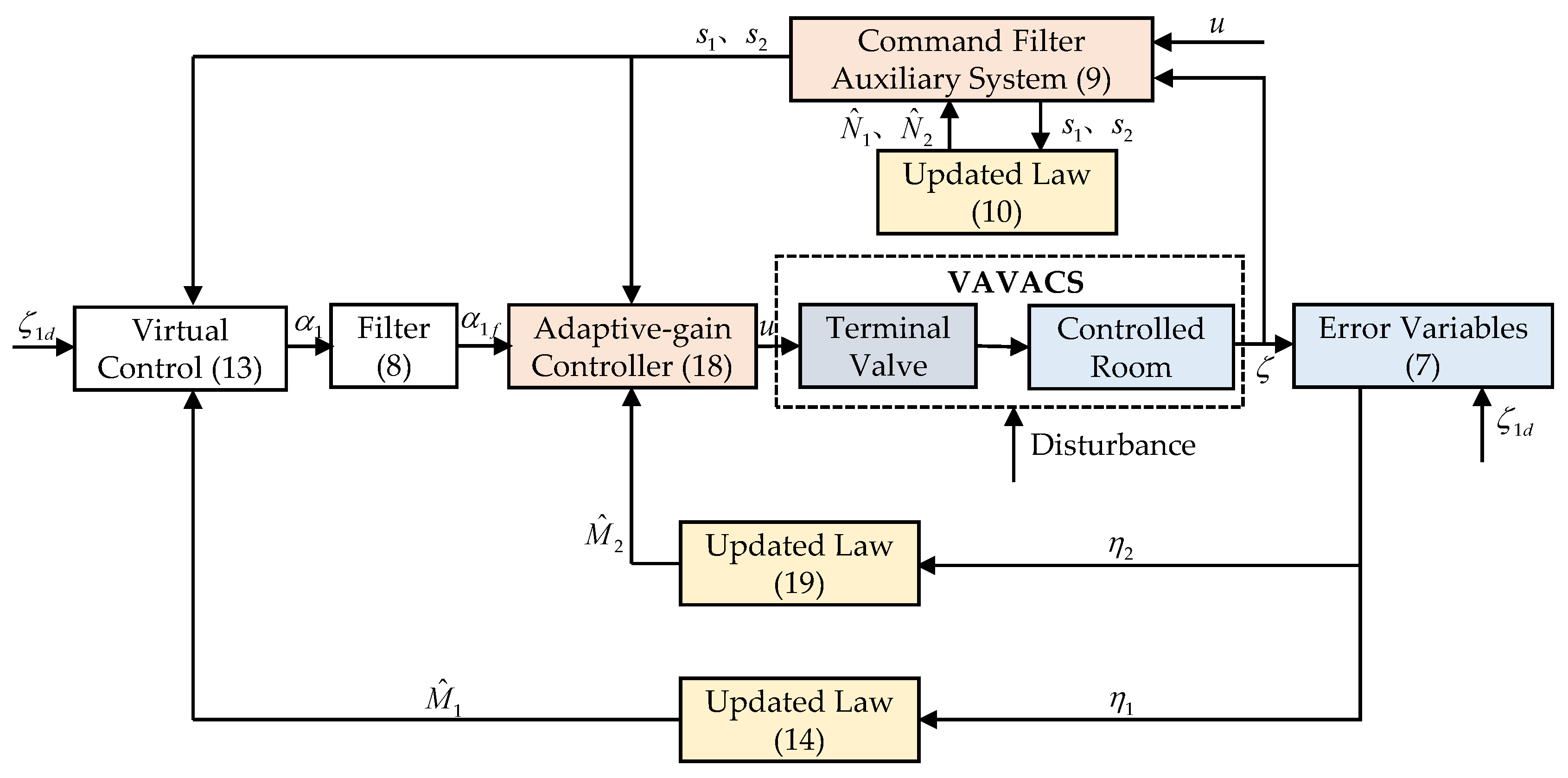
3. Command Filter-Based Adaptive-Gain Controller Design

In this section, a command filter-based adaptive-gain controller is presented to achieve the temperature tracking of the variable air volume air-conditioning system (VAVACS), where the updated gains relieve the conservatism of the controller gain selection.

3.1. Controller Design

Define

$$\{\begin{array}{l}{z}_1={\zeta }_1-{\zeta }_{1d},z_2={\zeta }_2-{\alpha }_{1f}\\ {\eta }_1=z_1-s_1,{\eta }_2=z_2-s_2\end{array}$$

(7)

where $z_1$ represents the tracking error; ${\zeta }_{1d}$ represents the temperature command; ${\alpha }_1$ represents the virtual control; ${\alpha }_{1f}$ represents the filtered signal of ${\alpha }_1$; and $s_1$ and $s_2$ represent the auxiliary signals introduced later.

To obtain the filtering variable ${\alpha }_{1f}$, the following command filter is adopted:

$${\dot{\alpha }}_{1f}=-w_1({\alpha }_{1f}-{\alpha }_1),{\alpha }_{1f}(0)={\alpha }_1(0)$$

(8)

with $w_1>0$ denoting the adjustable filter parameter.

To eliminate the effect of the filtered error ${\epsilon }_1={\alpha }_{1f}-{\alpha }_1$ and the input delay on temperature tracking, an adaptive-gain auxiliary system was designed as follows:

$$\{\begin{array}{l}{\dot{s}}_1=-k_1{s}_1+g_1{s}_2+g_1{\epsilon }_1-{\sigma }_1\\ {\dot{s}}_2=-k_2{s}_2-g_1{s}_1+g_{2}u(t-\tau )-g_{2}u(t)-{\sigma }_2\end{array}$$

(9)

in which $k_1>0$ and $k_2>0$ denote the adjustable controller parameters; ${\sigma }_i={\displaystyle \frac{g_i{s}_i{\widehat{N}}_i^2}{s_i{\widehat{N}}_i\tanh \left[s_i/h(t)\right]+h(t)}}$ ($i=1,2$), where the function $h(t)>0$ satisfies ${\displaystyle {\int }_0^{t}h}(\nu )\mathrm{d}\nu \le {\overline{h}}_1<+\infty$, with ${\overline{h}}_1>0$; $N_i>0$ being constants, updated by

$${\dot{\widehat{N}}}_i={\gamma }_i{g}_i\left|s_i\right|,i=1,2$$

(10)

with ${\gamma }_1>0$ and ${\gamma }_2>0$ being the designed parameters.

Step 1: In using (4) and (7), differentiating ${\eta }_1$ yields

$$\begin{array}{ll}{\dot{\eta }}_1& ={\dot{z}}_1-{\dot{s}}_1\\ & =g_1{\zeta }_2+Q_r/c_r+d_1(t)-{\dot{\zeta }}_{1d}-{\dot{s}}_1\end{array}$$

(11)

Plugging (9) into (11) yields

$$\begin{array}{ll}{\dot{\eta }}_1& =g_1{\zeta }_2+Q_r/c_r+d_1(t)-{\dot{\zeta }}_{1d}-(-k_1{s}_1+g_1{s}_2+g_1{\epsilon }_1-{\sigma }_1)\\ & =g_1({\eta }_2+{\alpha }_1)+Q_r/c_r+d_1(t)-{\dot{\zeta }}_{1d}+k_1{s}_1+{\sigma }_1\end{array}$$

(12)

From (12), the virtual control ${\alpha }_1$ is designed as

$$\{\begin{array}{l}{\alpha }_1={\displaystyle \frac{{\alpha }_{1a}+{\alpha }_{1s}}{g_1}},{\alpha }_{1s}={\alpha }_{1s1}+{\alpha }_{1s2}\\ {\alpha }_{1a}={\dot{\zeta }}_{1d}-Q_r/c_r-k_1{s}_1-{\sigma }_1\\ {\alpha }_{1s1}=-k_1{\eta }_1,{\alpha }_{1s2}={\displaystyle \frac{-{\eta }_1{\widehat{M}}_1^2}{{\eta }_1{\widehat{M}}_1\tanh [{\eta }_1/h(t)]+h(t)}}\end{array}$$

(13)

where $M_1>0$ denotes the unknown constant parameter, and its estimated value is updated as follows:

$${\dot{\widehat{M}}}_1={\mu }_1\left|{\eta }_1\right|$$

(14)

with ${\mu }_1>0$. Putting (13) into (12), one has

$${\dot{\eta }}_1=-k_1{\eta }_1+g_1{\eta }_2+{\alpha }_{1s2}+d_1(t)$$

(15)

Step 2: In using (4) and (7), differentiating ${\eta }_2$ yields

$${\dot{\eta }}_2=g_{2}u(t-\tau )-K{\zeta }_2+d_2(t)-{\dot{\alpha }}_{1f}-{\dot{s}}_2$$

(16)

Plugging (9) into (16) yields

$$\begin{array}{ll}{\dot{\eta }}_2& =g_{2}u(t-\tau )-K{\zeta }_2+d_2(t)-{\dot{\alpha }}_{1f}-[-k_2{s}_2-g_1{s}_1+g_{2}u(t-\tau )-g_{2}u(t)-{\sigma }_2]\\ & =g_{2}u(t)-K{\zeta }_2+d_2(t)-{\dot{\alpha }}_{1f}+g_1{s}_1+k_2{s}_2+{\sigma }_2\end{array}$$

(17)

Therefore, the controller input was designed as follows:

$$\{\begin{array}{l}u={\displaystyle \frac{(u_a+u_s)}{g_2}},u_s=u_{s1}+u_{s2}\\ u_a=K{\zeta }_2+{\dot{\alpha }}_{1f}-g_1{s}_1-k_2{s}_2-{\sigma }_{22}-g_1{\eta }_1\\ u_{s1}=-k_2{\eta }_2,u_{s2}=-{\displaystyle \frac{{\eta }_2{\widehat{M}}_2^2}{{\eta }_2{\widehat{M}}_2\tanh [{\eta }_2/h(t)]+h(t)}}\end{array}$$

(18)

where $M_2>0$ denotes the unknown constant, updated as

$${\dot{\widehat{M}}}_2={\mu }_2\left|{\eta }_2\right|$$

(19)

with ${\mu }_2>0$. Putting (18) into (17), one has

$${\dot{\eta }}_2=-k_2{\eta }_2+u_{s2}-g_1{\eta }_1+d_2(t)$$

(20)

The control framework of the VAVACS is presented in Figure 2.

3.2. Stability Analysis

Theorem 1.

With Assumption 1, adaptive laws (10), (14) and (19) and control law (18) and in choosing the suitable controller parameters $k_1$, $k_2$, $w_1$, ${\gamma }_1$, ${\gamma }_2$, ${\mu }_1$ and ${\mu }_2$, it can be gained that both the boundedness of all the system signals and the asymptotic tracking performance are assured.

Proof. 

See Appendix A. □

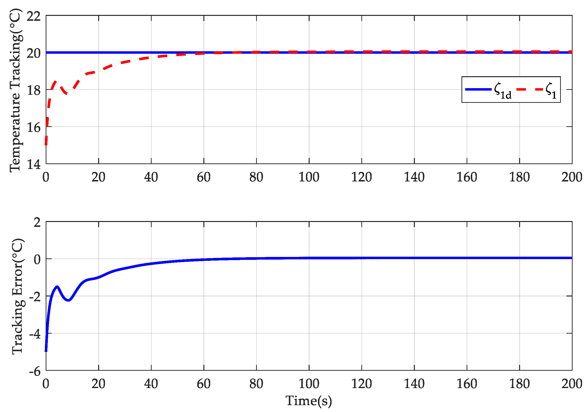
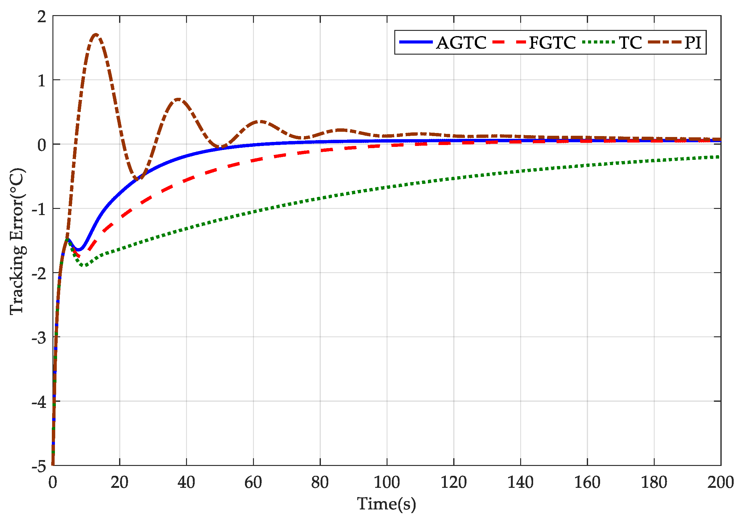
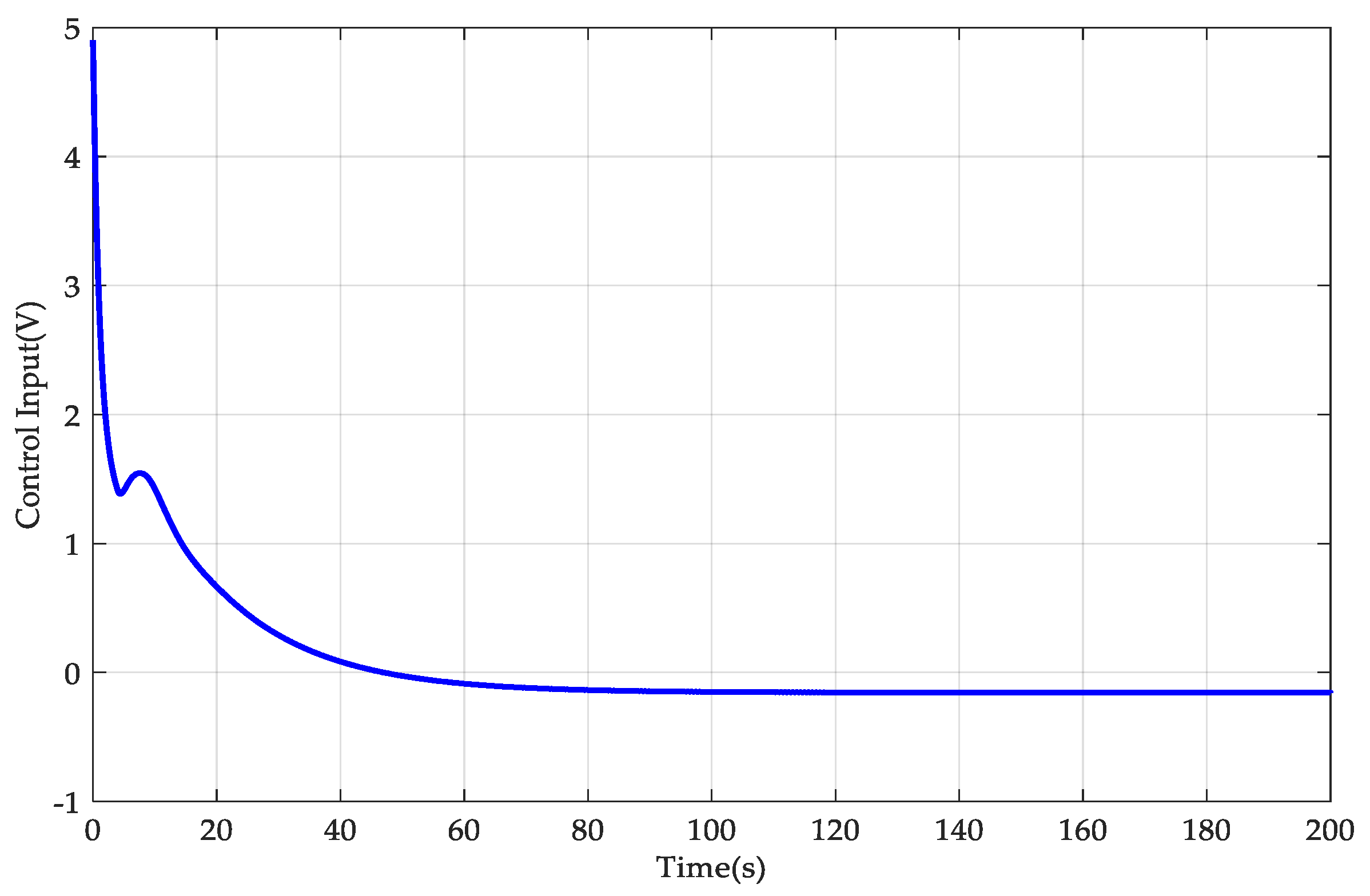
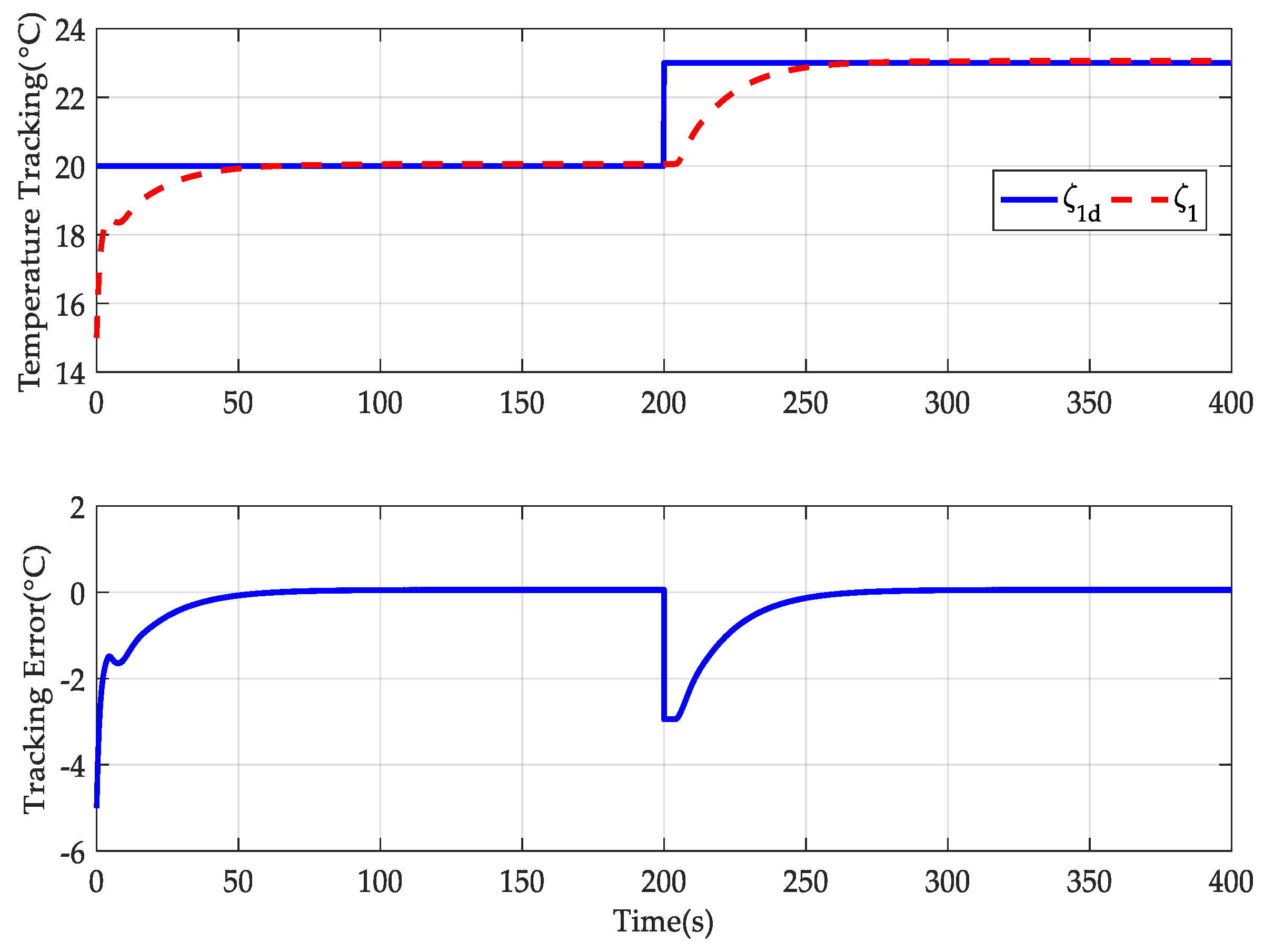
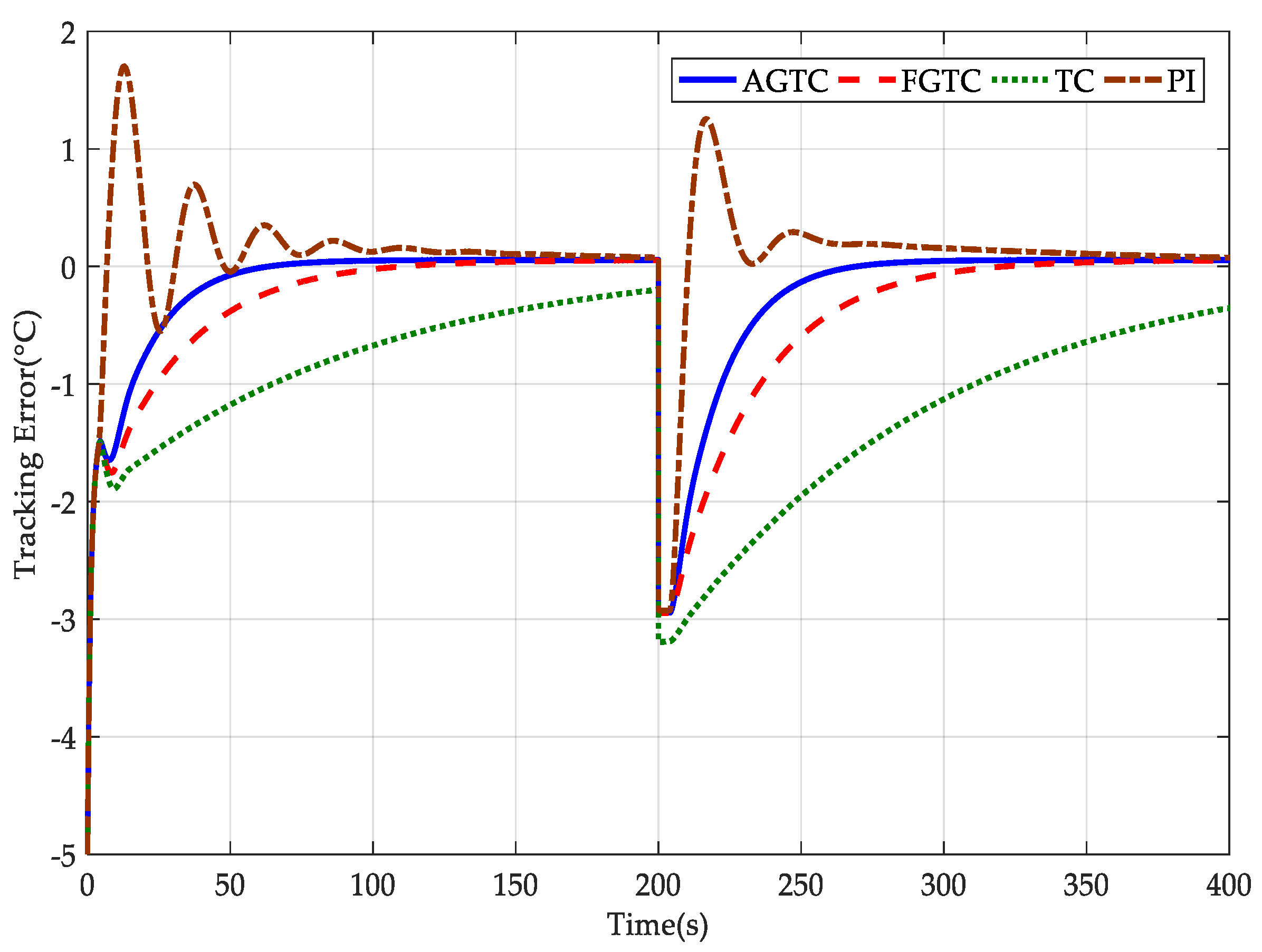
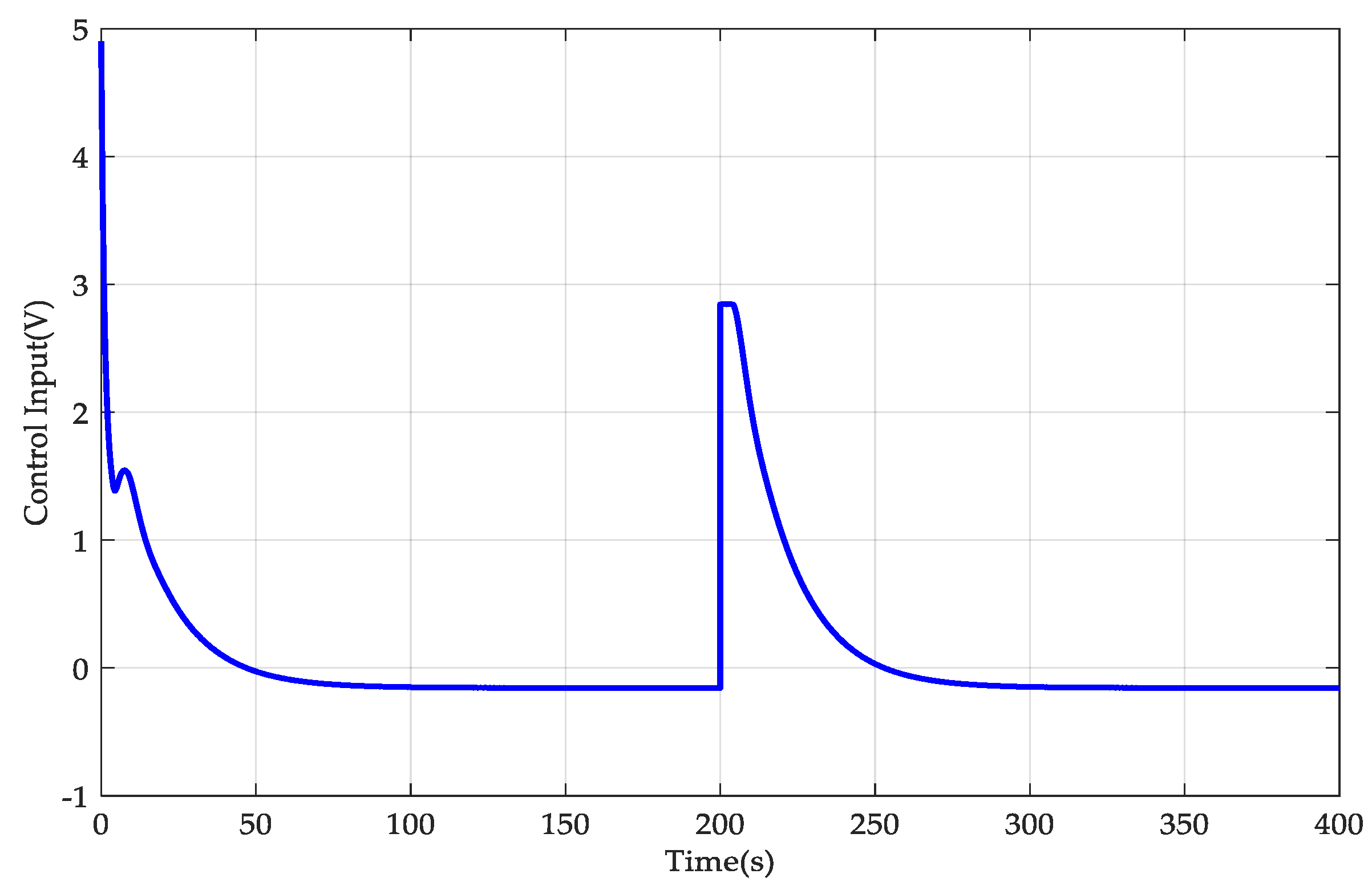
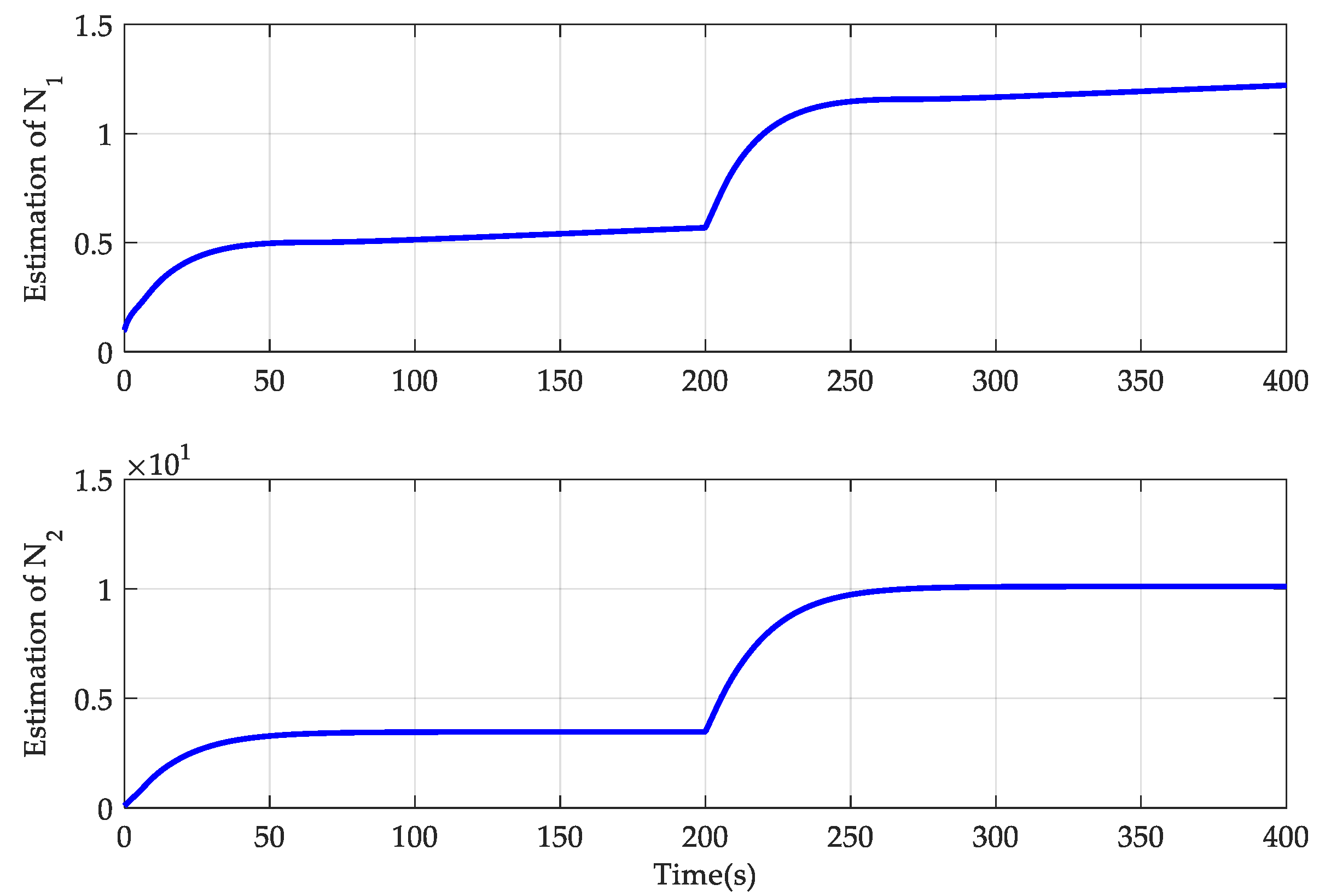
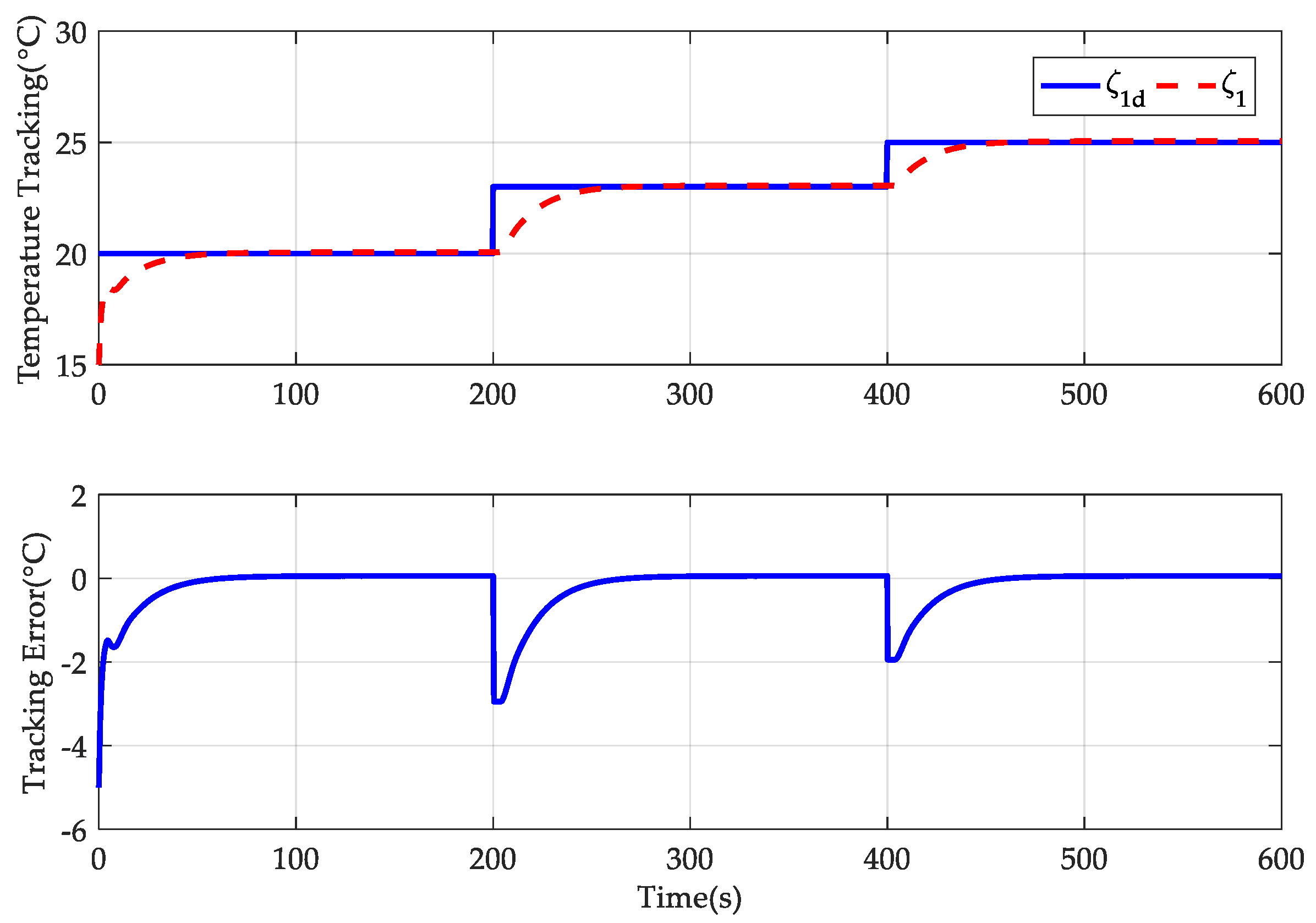
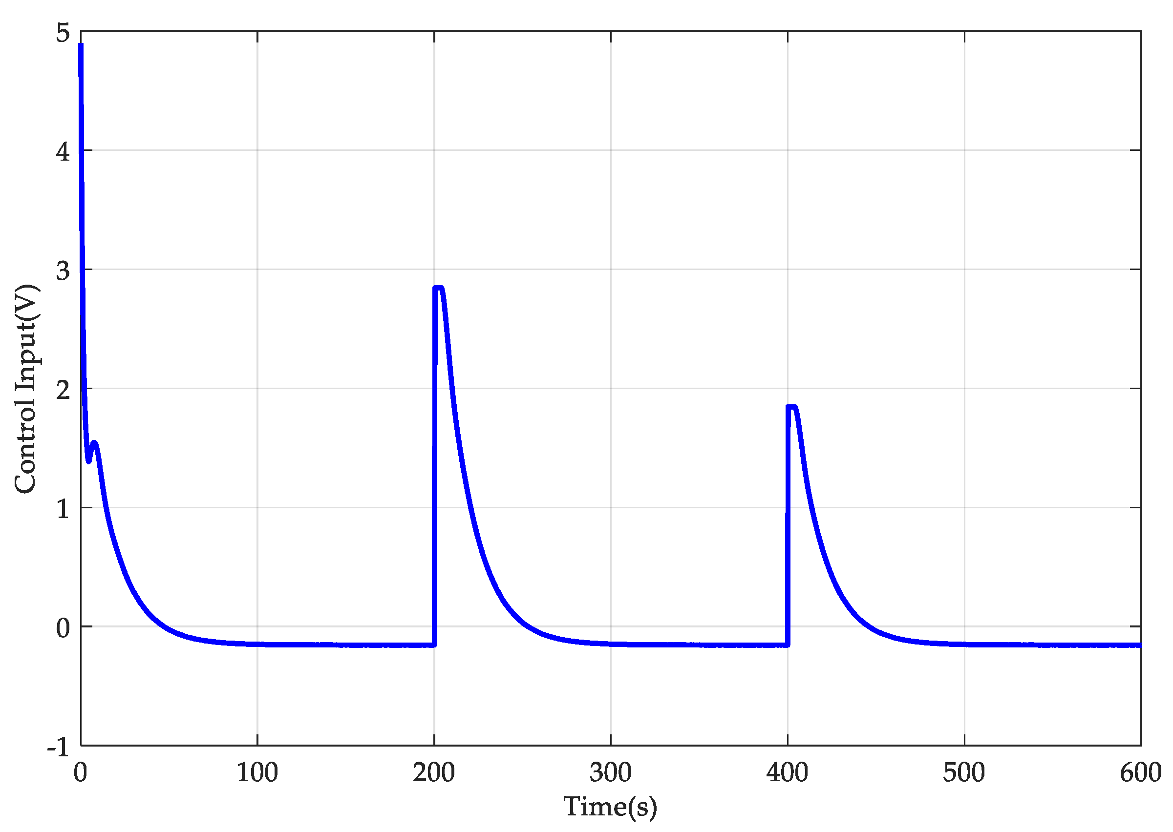
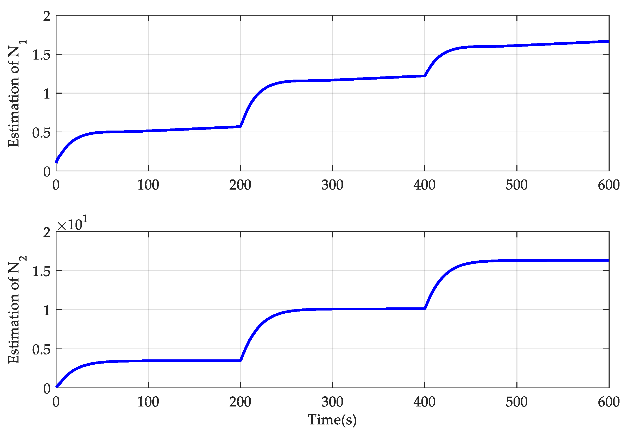
4. Simulation Results

The actual parameters of the VAVACS and the controlled room are shown in

Table 1. Physical parameters of the VAVACS and the controlled room.

Parameter	Value	Parameter	Value
$c_s$ (J/°C)	1 × 104	c (J/kg/°C)	1.2 × 103
$\rho$ (kg/m3)	1.1	Qr (W)	3.5 × 103
Vr (m3)	4 × 101	Ts (°C)	3 × 101
$k_a{k}_v$ (m/s/V)	0.58	K (s−1)	0.82

. The input delay $\tau$ was set as $\tau =4$ s. $T_n(0)=15°\mathrm{C}$. The disturbances were set as $f_1(t)=500\sin (10t)$$\mathrm{W}$ and $f_2(t)=0.1\sin (3t)$ m/s.

The following controllers are compared:

(1)

AGTC: The adaptive-gain temperature controller was developed here, and its controller parameters are provided by $k_1=1$, $k_2=0.05$, $w_1=1000$, ${\gamma }_1=0.1$, ${\gamma }_2=0.5$, ${\mu }_1=0.0001$ and ${\mu }_2=0.00002$. The other parameters were set as ${\widehat{N}}_1(0)=0.3$, ${\widehat{N}}_2(0)=0.2$, ${\widehat{M}}_1(0)=0.1$ and ${\widehat{M}}_1(0)=0.1$. Also, $h(t)=1/(t^2+300)$.

(2)

FGTC: This is a fixed-gain temperature controller. The difference between the AGTC and FGTC is that a fixed controller gain technique is introduced into the FGTC. That is, ${\gamma }_1={\gamma }_2=0$ and ${\mu }_1={\mu }_2=0$ in the FGTC.

(3)

TC: This is a temperature controller without input delay compensation. The difference between the TC and FGTC is that the input delay is not compensated in the TC.

(4)

PI: This is a proportional–integral controller. The controller parameters were set as $k_p=2$ and $k_i=0.5$.

Case 1: First, a case in which the temperature command was set as 20 °C was carried out to test the tracking performance of the exploited controller. The temperature tracking performance of the AGTC is presented in Figure 3. The contrastive tracking errors of the four controllers can be observed in Figure 4. It is not difficult to find that AGTC developed in this study obtains both the asymptotic convergence performance and the best temperature control performance among the four controllers, where the steady accuracy of the AGTC decreases by about 25%, 41% and 72% when compared to those of the FGTC, TC and PI. This is owed to the input delay compensation method and the adaptive gain technique introduced into the AGTC. Given the usage of the fixed-gain technique in the FGTC, the FGTC achieves the worse temperature tracking performance when compared to the AGTC, which uncovers the validity of the adaptive-gain method utilized in the AGTC. The temperature control performance of the FGTC is better than that of the TC, which reveals the effectiveness of the input delay compensation approach in the FGTC. Moreover, it is observed that the temperature tracking performance of PI is superior to that of the TC. This uncovers that PI adopts a certain robust ability against input delay and disturbances via using high feedback gains, whereas for lack of using the input delay compensation method and the adaptive-gain technique, PI obtains the worse temperature control performance when comparing with the AGTC and FGTC. This demonstrates the effectiveness of the input delay compensation method and the adaptive-gain technique in the AGTC. Also, the control input of the AGTC can be observed in Figure 5, which is smooth and bounded. The estimation values of N_i and M_i (i = 1, 2) in the AGTC, presented in Figure 6 and Figure 7, can gradually converge, which shows the validity of the adaptive-gain technique in the AGTC.

Case 2: To further test the tracking performance of the exploited controller, a new case was considered. The contrastive simulation results are collected in Figure 8, Figure 9, Figure 10, Figure 11 and Figure 12. It is easy to find that the AGTC achieves the best temperature control performance when compared to the other ones. This demonstrates the effectiveness of the input delay compensation method and the adaptive-gain technique in the AGTC. Also, the control input of the AGTC can be observed in Figure 10, which is smooth and bounded.

The estimation values of N_i and M_i (i = 1, 2) in the AGTC presented in Figure 11 and Figure 12 can gradually converge. Therefore, the advantages of the developed approach are revealed once again.

Case 3: Finally, another case was considered to further test the tracking performance of the developed control method. The contrastive simulation results are collected in Figure 13, Figure 14, Figure 15, Figure 16 and Figure 17. As observed, the temperature control performance of the AGTC still precedes the other ones. This is owing to the input delay compensation method and the adaptive gain technique introduced into the AGTC. Given the usage of the fixed-gain technique in the FGTC, the FGTC gains the worse temperature tracking performance again when compared to the AGTC, which uncovers the validity of the adaptive-gain method utilized in the AGTC. The temperature control performance of the FGTC is better than that of the TC, which reveals the effectiveness of the input delay compensation approach in the FGTC. The above-mentioned facts demonstrate the advantages of the developed approach once again. Also, the control input of the AGTC can be observed in Figure 15, which is still smooth and bounded. The estimation values of N_i and M_i (i = 1, 2) in the AGTC presented in Figure 16 and Figure 17 can gradually converge as well.

5. Conclusions

In this study, an adaptive-gain command filter control framework was exploited for the room temperature of variable air volume air-conditioning systems, where an adjusted gain technique was introduced into the control framework to compensate for parametric uncertainties, matched disturbances and mismatched disturbances. This makes the conservatism of the controller gain selection relaxed. Through adopting the Lyapunov theory, the asymptotic tracking performance for the room temperature can be assured with the controller presented. Finally, the contrastive simulation results demonstrate the validity of the developed method, in which the steady accuracy of the AGTC decreases by about 25%, 41% and 72% when compared to those of the FGTC, TC and PI. In future research, it is worth studying a reinforcement learning-based control approach for the room temperature of variable air volume air-conditioning systems to optimize the control performance and achieve the self-tuning process of controller parameters.

References

- Okochi, G.S.; Yao, Y. A Review of Recent Developments and Technological Advancements of Variable-Air-Volume (VAV) Air-Conditioning Systems. Renew. Sustain. Energy Rev. 2016, 59, 784–817. [Google Scholar] [CrossRef]
- Vashisht, S.; Rakshit, D. Recent Advances and Sustainable Solutions in Automobile Air Conditioning Systems. J. Clean. Prod. 2021, 329, 129754. [Google Scholar] [CrossRef]
- Li, W.; Gong, G.; Ren, Z.; Ouyang, Q.; Peng, P.; Chun, L.; Fang, X. A Method for Energy Consumption Optimization of Air Conditioning Systems Based on Load Prediction and Energy Flexibility. Energy 2022, 243, 123111. [Google Scholar] [CrossRef]
- Al-Yasiri, Q.; Szabó, M.; Arıcı, M. A Review on Solar-Powered Cooling and Air-Conditioning Systems for Building Applications. Energy Rep. 2022, 8, 2888–2907. [Google Scholar] [CrossRef]
- Chen, J.; Zhang, L.; Li, Y.; Shi, Y.; Gao, X.; Hu, Y. A Review of Computing-Based Automated Fault Detection and Diagnosis of Heating, Ventilation and Air Conditioning Systems. Renew. Sustain. Energy Rev. 2022, 161, 112395. [Google Scholar] [CrossRef]
- Zhang, Y.; Yan, T.; Xu, X.; Gao, J.; Huang, G. Room Temperature and Humidity Decoupling Control of Common Variable Air Volume Air-Conditioning System Based on Bilinear Characteristics. Energy Built Environ. 2023, 4, 354–367. [Google Scholar] [CrossRef]
- Li, D.; Ahmat, M.; Cao, H.; Di, F. Optimization of Double-Closed-Loop Control of Variable-Air-Volume Air-Conditioning System Based on Dynamic Response Model. Buildings 2024, 14, 677. [Google Scholar] [CrossRef]
- Mohammed, J.A.K.; Mohammed, F.M.; Jabbar, M.A.S. Investigation of High Performance Split Air Conditioning System by Using Hybrid PID Controller. Appl. Therm. Eng. 2018, 129, 1240–1251. [Google Scholar] [CrossRef]
- Xie, Y.; Yang, P.; Qian, Y.; Zhang, Y.; Li, K.; Zhou, Y. A Two-Layered Eco-Cooling Control Strategy for Electric Car Air Conditioning Systems with Integration of Dynamic Programming and Fuzzy PID. Appl. Therm. Eng. 2022, 211, 118488. [Google Scholar] [CrossRef]
- Nasirpour, N.; Balochian, S. Optimal Design of Fractional-Order PID Controllers for Multi-Input Multi-Output (Variable Air Volume) Air-Conditioning System Using Particle Swarm Optimization. Intell. Build. Int. 2017, 9, 107–119. [Google Scholar] [CrossRef]
- Li, S.; Wei, M.; Wei, Y.; Wu, Z.; Han, X.; Yang, R. A Fractional Order PID Controller Using MACOA for Indoor Temperature in Air-Conditioning Room. J. Build. Eng. 2021, 44, 103295. [Google Scholar] [CrossRef]
- Zhao, B.Y.; Zhao, Z.G.; Li, Y.; Wang, R.Z.; Taylor, R.A. An Adaptive PID Control Method to Improve the Power Tracking Performance of Solar Photovoltaic Air-Conditioning Systems. Renew. Sustain. Energy Rev. 2019, 113, 109250. [Google Scholar] [CrossRef]
- Shi, S.; Miyata, S.; Akashi, Y.; Momota, M.; Sawachi, T.; Gao, Y. Model-Based Optimal Control Strategy for Multizone VAV Air-Conditioning Systems for Neutralizing Room Pressure and Minimizing Fan Energy Consumption. Build. Environ. 2024, 256, 111464. [Google Scholar] [CrossRef]
- Yang, X.; Ge, Y.; Deng, W.; Yao, J. Observer-Based Motion Axis Control for Hydraulic Actuation Systems. Chin. J. Aeronaut. 2023, 36, 408–415. [Google Scholar] [CrossRef]
- Rsetam, K.; Al-Rawi, M.; Al-Jumaily, A.M.; Cao, Z. Finite Time Disturbance Observer Based on Air Conditioning System Control Scheme. Energies 2023, 16, 5337. [Google Scholar] [CrossRef]
- Kamalapurkar, R.; Fischer, N.; Obuz, S.; Dixon, W.E. Time-Varying Input and State Delay Compensation for Uncertain Nonlinear Systems. IEEE Trans. Automat. Contr. 2016, 61, 834–839. [Google Scholar] [CrossRef]
- Yang, X.; Ge, Y.; Deng, W.; Yao, J. Command Filtered Adaptive Tracking Control of Nonlinear Systems with Prescribed Performance under Time-Variant Parameters and Input Delay. Int. J. Robust Nonlinear Control 2023, 33, 2840–2860. [Google Scholar] [CrossRef]
- Na, J.; Huang, Y.; Wu, X.; Su, S.F.; Li, G. Adaptive Finite-Time Fuzzy Control of Nonlinear Active Suspension Systems with Input Delay. IEEE Trans. Cybern. 2020, 50, 2639–2650. [Google Scholar] [CrossRef] [PubMed]
- Li, D.-P.; Liu, Y.-J.; Tong, S.; Chen, C.L.P.; Li, D.-J. Neural networks-based adaptive control for nonlinear state constrained systems with input delay. IEEE Trans. Cybern. 2019, 49, 1249–1258. [Google Scholar] [CrossRef] [PubMed]
- Yang, Z.; Zhang, X.; Zong, X.; Wang, G. Adaptive fuzzy control for non-strict feedback nonlinear systems with input delay and full state constraints. J. Frankl. Inst. 2020, 357, 6858–6881. [Google Scholar] [CrossRef]
- Ma, J.; Xu, S.; Zhuang, G.; Wei, Y.; Zhang, Z. Adaptive Neural Network Tracking Control for Uncertain Nonlinear Systems with Input Delay and Saturation. Int. J. Robust Nonlinear Control 2020, 30, 2593–2610. [Google Scholar] [CrossRef]
- Ma, J.; Xu, S.; Ma, Q.; Zhang, Z. Event-Triggered Adaptive Neural Network Control for Nonstrict-Feedback Nonlinear Time-Delay Systems with Unknown Control Directions. IEEE Trans. Neural Netw. Learn. Syst. 2020, 31, 4196–4205. [Google Scholar] [CrossRef]
- Zhou, Y.; Wang, X.; Xu, R. Command-Filter-Based Adaptive Neural Tracking Control for a Class of Nonlinear MIMO State-Constrained Systems with Input Delay and Saturation. Neural Netw. 2022, 147, 152–162. [Google Scholar] [CrossRef]
- Zhu, Z.; Liang, H.; Liu, Y.; Xue, H. Command Filtered Event-Triggered Adaptive Control for MIMO Stochastic Multiple Time-Delay Systems. Int. J. Robust Nonlinear Control 2022, 32, 715–736. [Google Scholar] [CrossRef]
- Yang, X.; Ge, Y.; Deng, W.; Yao, J. Precision Motion Control for Electro-Hydraulic Axis Systems under Unknown Time-Variant Parameters and Disturbances. Chin. J. Aeronaut. 2024, 37, 463–471. [Google Scholar] [CrossRef]
- Krstic, M.; Kanellakopoulos, I.; Kokotovic, P. Nonlinear and Adaptive Control Design; Wiley: New York, NY, USA, 1995. [Google Scholar]
- Yang, X.; Deng, W.; Yao, J. Neural Adaptive Dynamic Surface Asymptotic Tracking Control of Hydraulic Manipulators with Guaranteed Transient Performance. IEEE Trans. Neural Netw. Learn. Syst. 2023, 34, 7339–7349. [Google Scholar] [CrossRef] [PubMed]