Point and Interval Forecasting of Coal Price Adopting a Novel Decomposition Integration Model

Abstract

Accurate and trustworthy forecasting of coal prices can offer theoretical support for the rational planning of coal industry output, which is of great importance in ensuring a stable and sustainable energy supply and in achieving carbon neutrality targets. This paper proposes a novel decomposition integration model, called VCNQM, to perform point and interval forecasting of coal price by a combination of variational modal decomposition (VMD), chameleon swarm algorithm (CSA), N-BEATS, and quantile regression. Initially, the variational modal decomposition is enhanced by the chameleon swarm algorithm for decomposing the coal price sequence. Then, N-BEATS is used to forecast each subsequence of coal prices, integrating all results to obtain a point forecast of coal prices. Next, interval forecasting of coal prices is achieved through quantile regression. Finally, to demonstrate the superiority of the VCNQM model’s prediction, we make a cross-comparison about predictive performance between the VCNQM model and other benchmark models. According to the experimental findings, we demonstrate the following: after the decomposition by CSA-VMD, the coal price subseries’ fluctuation is significantly weakened; using quantile regression provides a reliable interval prediction, which is superior to point prediction; the predicted interval coverage probability (PICP) is higher than the confidence level of 90%; the share power industry index and coal industry index have the greatest impact on coal prices in China; compared to these benchmark models, the VCNQM model’s prediction errors are all reduced. Therefore, we conclude that when forecasting coal prices, the VCNQM model has an accurate and reliable prediction.

1. Introduction

As a fundamental element of the national economy and social development, coal plays a crucial strategic role across the entire socioeconomic system in China. However, currently affected by the growing domestic coal demand and the increasing scarcity of imported coal resources from abroad, coal prices have become increasingly volatile, adversely affecting the stable development of China’s macroeconomy. Given this context, scientific prediction of China’s coal prices will facilitate the Chinese government to foresee market trend and make timely adjustments to energy reserves and import strategies, maintaining China’s energy security and sustainable development [1,2]. In addition, by accurately forecasting coal prices, coal companies and industries can optimize their production plans, control operating costs, and improve their market competitiveness [3]. At the same time, it also helps investors make smarter decisions and avoid market risks. On the premise of taking into account the non-stable and non-linear characteristics of coal price sequences, the majority of current research has adopted the decomposition integration model to forecast coal prices. The hybrid model consists of two parts, including decomposition and integration. The decomposition phase splits the complex raw signal of coal prices into some simple sub-signals, and then develops predictions for each sub-signal separately. The integration phase integrates each sub-signal prediction to obtain the final result. In summary, coal price forecasting is not only an essential topic for academic research, but also an important support for formulating energy policies, promoting the stable development of the domestic economy and coal industry [4]. Therefore, in-depth research and improvement of coal price forecasting methods have considerable theoretical value and practical significance. Following this theory, this paper proposes a new decomposition integration model (VCNQM) with improvements in the decomposition phase.

Presently, coal price forecasting models are mainly divided into single and hybrid models.

Early scholars mostly used a single model to predict coal prices. Single models mainly include traditional statistical models and machine learning algorithms. In the case of traditional statistical models, several models, such as the dynamic factor model, the VAR model, the ARIMA model, have been applied to predict energy price, including coal, gas, and so on [5,6,7,8]. However, traditional statistical models are only suitable for dealing with smooth or post-differential smooth time sequences when predicting coal prices, so they cannot properly handle the non-linear and non-stable characteristics of coal price sequences. Consequently, researchers started to employ machine learning algorithms to predict coal prices, including conventional machine learning algorithms and deep learning algorithms. In the case of conventional machine learning algorithms, when making long-term predictions for energy sources such as coal, Herrera et al. [9] compared the results of machine learning algorithms such as artificial neutral network and random forests to traditional econometric methods, demonstrating that machine learning algorithms outperformed the traditional econometric methods. Bonita and Muflikhah [10] utilized a support vector regression machine (SVR) and obtained the forecasting results of coal price with a low error. In the case of deep learning algorithms, Fan et al. [11] utilized a multi-layer perceptron network (MLP) to predict coal price trends. Compared with the ARIMA model, MLP can better identify the non-linear characteristics of coal price time sequences and has higher forecasting accuracy and greater fitness. Matyjaszeka et al. [12] investigated the predictive performance of the generalized regression neural network (GRNN) and showed that based on full-time series, its predictive performance is better than that of the ARIMA model and the robust model. Although conventional machine learning algorithms, such as MLP and GRNN, can compensate for the disadvantages of traditional statistical models. which need to follow assumptions such as smooth time series, they are unable to capture the dynamic rules of time series. Chen et al. [13] considered that wind speed data are as non-linear as coal price and applied the recurrent neural network (RNN), the LSTM network, and the gated recurrent unit (GRU) to forecast wind speed. Although RNN, and its variants LSTM, as well GRU make up for the shortcomings of the previous single model in predicting coal prices [14], they cannot effectively handle the high fluctuations in coal price series.

The multi-scale model combines the excellent features of several single models, and compared to a single model, its prediction accuracy and applicability are effectively improved [15]. To forecast the monthly changes in Australian power coal prices, Alameer et al. [16] proposed the LSTM-DNN model, which has better prediction accuracy and flexibility compared to the support vector machine model. Wang and Wang [17] created the DPFWR neural network based on the double parallel feedforward neural network, to forecast energy prices, such as Rotterdam coal. However, this type of multi-scale model does not diminish the noise of the original signals. Therefore, most scholars currently use decomposition integration models for prediction. In the signal decomposition phase, the representative methods are empirical modal decomposition (EMD) and variational modal decomposition (VMD). EMD is an adaptive time series decomposition technique, but it is limited by endpoint effects and modal decomposition confusion [18]. Therefore, scholars have proposed ensemble empirical modal decomposition [19] and complete ensemble empirical mode decomposition (CEEMDAN) [20] to enhance the decomposition by adding white noise and adaptive noise to the original time series, respectively. However, EEMD suffers from reconstruction errors and CEEMDAN suffers from residual noise and pseudo-modal problems in the decomposition. In view of the above, several researchers proposed a new decomposition method (ICEEMDAN) to decompose energy price signals, which effectively compensates for the shortcomings of the original EMD and its variants [21,22], but the restructuring of the high-frequency intrinsic mode function (IMF) will indirectly lead to a reduction in forecasting accuracy, posing a huge challenge to short-term forecasting. Both Rayi et al. [23] and Li et al. [24] noted that VMD is more widely applicable than other signal decomposition techniques such as EMD and its variants, and overcomes the shortcomings of other decomposition techniques. To estimate future coal prices, Zhang et al. [25] proposed a new hybrid model called VMD-A-LSTM-SVR, in which the quadratic penalty factor α was determined by empirical judgment, and the hybrid model had a more accurate prediction than LSTM and SVR. In addition, to predict crude oil prices, several researchers have combined VMD with other methods, such as sample entropy (SE) and GRU, an attention mechanism and GRU, the support vector machine and ARIMA [26,27,28]. However, the accuracy of the decomposition results cannot be guaranteed by using empirical judgment to determine α and the number of decomposition modes N. Wu et al. [29] applied an arithmetic optimization algorithm to enhance VMD’s decomposition capacity and used the fitness function to determine the VMD parameters, offering a new solution to decompose coal price series effectively.

Point predictions of coal prices were the focus of the aforementioned studies. Considering the fact that point predictions only offer a single forecast value, Ding et al. [30] proposed a C-MIDAS-X hybrid model and applied kernel density estimation (KDE) to obtain probabilistic forecasts of coal prices. Probability density forecasts can cope with the high volatility of coal price series and the uncertainty of forecasts more effectively, providing uncertain information about future coal prices and a more practical reference for decision-makers [30]. However, the density function of using KDE for interval estimation is influenced by the width of the subinterval.

In summary, the existing studies on coal price forecasting still have the following areas that need improvement:

(1)

In the decomposition stage of a hybrid model, EMD and its variants are unable to effectively decompose the high volatile coal price series, being limited by various decomposition errors. In addition, when using VMD to decompose coal price series, the empirical judgment is not scientific enough. Therefore, there is still room for improvement in the decomposition stage.

(2)

The current academic research mainly focuses on point forecasting of coal prices, and the existing research on probabilistic forecasting mainly adopts kernel density estimation, whose result is vulnerable to the width of the subintervals. Therefore, probabilistic forecasting needs to be further supplemented.

In this paper, we refer to Wu et al. [29] in the decomposition phase, using the combination of variational modal decomposition and chameleon swarm algorithm (CSA) to decompose the coal price series. Next, we minimize the envelope entropy to find the optimal solution in a given range of parameters (N, α). Compared with highly respected meta-heuristic algorithms such as SSA [31] on most test functions, CSA has stronger exploration capability and higher development intensity, leading to optimal performance [32]. After that, we use quantile regression to optimize the N-BEATS, which can solve the probabilistic prediction problem under the unknown coal price distribution and compensate for the weakness of kernel density estimation being vulnerable to the width of the subinterval. The output of N-BEATS is more interpretable than that of traditional forecasting methods and has a state-of-the-art generalization capability [33]. Accordingly, this paper introduces the following innovations:

(1)

In the signal decomposition stage, using a meta-heuristic algorithm can be used to optimize the parameter of the VMD, improving the reasonableness of the decomposition, as well as the accuracy of the decomposition.

(2)

This paper proposes a new hybrid model that enables point and interval forecasts of Chinese coal prices. Specifically, this paper combines the optimized VMD with N-BEATS to achieve point forecasts of Chinese coal prices, and based on these forecasts, it uses quantile regression to achieve the probabilistic prediction of coal prices, compensating for the shortcomings of kernel density estimation.

(3)

This paper extends the interpretability of coal prices prediction. Combining the mean impact value algorithm (MIV) with N-BEATS, we solve the problem that N-BEATS cannot analyze the importance of drivers on coal price forecasting, increasing the extent of the hybrid model’s application.

Here’s how the remainder of the paper is laid out: in Section 2, we explain how the VCNQM model is built; in Section 3, we show how the drivers are chosen, data are collected, and the model’s settings are determined; in Section 4, we provide an empirical analysis of coal price forecasting; and in Section 5, we draw the main research conclusions from our study.

2. Methodology

Considering the thought of decomposition and integration as well as the data-driven notion, this paper proposes a relevant coal price forecasting framework to complete interval forecasting and the importance analysis of drivers. As shown in Figure 1, first, this paper improves VMD using the CSA algorithm, obtaining CSA-VMD to decompose coal price sequences; then, this paper uses N-BEATS to process each subsequence and integrates all results to obtain the point forecasts of coal prices; next, this paper applies quantile regression to process the prediction from the previous step to achieve interval forecasts; finally, this paper uses the MIV algorithm to analyze the influence of drivers on coal prices.

2.1. Coal Price Sequence Decomposition Method

2.1.1. Variational Modal Decomposition

Variational modal decomposition (VMD) is a variational method for decomposing signals [34]. The core of VMD can be summarized in three steps: (1) determining all sub-signals’ number $N$ and constructing the constrained variational problem to assess the bandwidth of a mode; (2) introducing an augmented Lagrangian function to convert the previous problem into an unconstrained one, focusing only on finding a solution for the saddle point; (3) constantly updating each component $u_k$ and the central frequencies ${\omega }_k$ until the iterative constraints are satisfied to obtain the saddle point, thus obtaining the valid decomposition components. The non-stationary and non-linear coal price sequences are decomposed into $N$-modal components $u_k$, $u_k={\displaystyle \left\{u_1,u_2,\cdots ,u_{\mathrm{N}}\right\}}$. More details can be found in Dragomiretskiy and Zosso [30].

2.1.2. Chameleon Swarm Algorithm

A brand-new metaheuristic method called the chameleon swarm algorithm (CSA) was proposed by Malik Shehadeh Braik in 2021 to solve global numerical optimization problems [32]. CSA has mathematically modeled and implemented the chameleons’ behavior in searching for food, with the following main process:

• (1) Tracking the prey.

As chameleons search for prey in the desert and trees, their position is changing. The mathematical model of updating the chameleons’ position is as follows:

$$y_{ij}^{\overline{t}+1}=\left\{\begin{array}{ll}{y}_{ij}^{\overline{t}}+\mu \left(r_3\left(u{b}_j-l{b}_j\right)+l{b}_j\right)\mathrm{sgn}\left(rand-0.5\right)& r_i<P_p\\ y_{ij}^{\overline{t}}+p_1{r}_2\left(P_{ij}^{\overline{t}}-G_j^{\overline{\mathrm{t}}}\right)+p_2{r}_1\left(G_j^{\overline{\mathrm{t}}}-y_{ij}^{\overline{t}}\right)& r_i\ge P_p\end{array}\right.$$

(1)

where $i$, $j$, $\overline{t}$, and $T$ denote the chameleon, the number of dimensions, the number of iterations, and the maximum number of iterations, respectively, $y_{ij}^{\overline{t}}$ denotes the position of the chameleon, $u{b}_j$ and $l{b}_j$ denote the upper and lower bounds of the current dimension, $P_{ij}^{\overline{t}}$ denotes the chameleon’s best position, $G_j^{\overline{t}}$ denotes the global best position of the chameleon group, both $p_1$ and $p_2$ reflect the chameleon’s exploration capability, which are represented by two positive numbers, $r_i$ obeys the uniform distribution in the range of [0, 1], $i=\{1,2,3\}$, $P_p$, which is set to 0.1, denotes the likelihood that the chameleon will notice its prey, $\mathrm{sgn}\left(rand-0.5\right)$ represents the direction of rotation, $\mathrm{sgn}\left(rand-0.5\right)=\pm 1$, $\mu$ is the parameter of the search capability, $\mu =e^{{\left(-\alpha \overline{t}/T\right)}^3}$, $\alpha$ is a sensitive parameter, which is equal to 3.5.

• (2) Locating the prey.

The chameleons’ eyes have the feature of rotating and focusing independently, which help them identify and locate their prey over 360 degrees and update its position according to their prey’s position. The mathematical model of locating the prey is as follows:

$$y_i^{\overline{t}+1}=M\times \left(y_i^{\overline{t}}-{\overline{y}}_{\mathrm{i}}^{\overline{t}}\right)+{\overline{y}}_i^{\overline{t}}$$

(2)

$$M=R\left(\psi ,{\overrightarrow{V}}_{z_1,z_2}\right)$$

(3)

$$\psi =r\times \mathrm{sgn}\left(rand-0.5\right)\times \pi$$

(4)

where $y_i^{\overline{t}+1}$ is a chameleon’s new position after rotation, $y_i^{\overline{t}}$ represents the current position of the chameleon at iteration $\overline{t}$, ${\overline{y}}_i^{\overline{t}}$ is the center of $y_i^{\overline{t}}$, $M$ represents a rotation matrix, ${\overrightarrow{V}}_{z_1,z_2}$ is the orthogonal matrix formed by two standard orthogonal vectors $z_1$ and $z_2$, $R$ is the generation process of the rotation matrix, which is detailed in Braik [32], $\psi$ is the parameter of the chameleon’s rotation angle, in the range of [−$\pi$, $\pi$].

• (3) Capturing the prey.

When it is closest to the prey, the location of the chameleon changes slightly due to its tongue extending to attack the prey. When attacking the prey, the mathematical model of the velocity of the tongue and the change in position of the chameleon is as follows:

$$v_{ij}^{\overline{t}+1}=\omega \times v_{ij}^{\overline{t}}+c_1{r}_1\left(G_{\mathrm{j}}^{\overline{t}}-y_{ij}^{\overline{t}}\right)+c_2{r}_2\left(P_{ij}^{\overline{t}}-y_{ij}^{\overline{t}}\right)$$

(5)

$$y_{ij}^{\overline{t}+1}=y_{ij}^{\overline{t}}+{\displaystyle \frac{{\left(v_{ij}^{\overline{t}}\right)}^2-{\left(v_{ij}^{\overline{t}-1}\right)}^2}{2a}}$$

(6)

where $v_{ij}^{\overline{t}}$ and $v_{ij}^{\overline{t}+1}$ are the new attacking speed of the chameleon at iteration $\overline{t}$ and $\overline{t}+1$, respectively, $y_{ij}^{\overline{t}+1}$ and $y_{ij}^{\overline{t}}$ are the position of the chameleon at the respective iteration, $P_{ij}^{\overline{t}}$ represents the best position of the chameleon, $G_j^{\overline{t}}$ represents the global position of the chameleon swarm, $c_1$ and $c_2$ are two positive constants that control the effect of $P_{ij}^{\overline{t}}$ and $G_j^{\overline{t}}$ on the elongation of the chameleon’s tongue, $r_1$ and $r_2$ obey the uniform distribution in the range of [0, 1], $\omega$ is the inertia weight, ranging from 0 to 1, $a$ is the acceleration rate of the chameleon, $a=2590\times \left(1-e^{-\log \left(\overline{t}\right)}\right)$.

2.1.3. Hybrid Model for Coal Price Sequence Decomposition

Since artificially determining the parameters of VMD can hurt the decomposition, this paper proposes the CSA-VMD model to determine the parameters $(\alpha ,N)$ of VMD under the condition that the decomposition is optimal, using the minimum envelope entropy to assess the fitness of subseries and CSA to refine VMD. The magnitude of envelope entropy is positively proportional to the amount of noise contained in the modal component, and inversely proportional to the amount of information. The envelope entropy $E_A$ can be calculated by the following equation:

$$\left\{\begin{array}{c}{E}_A=-{\displaystyle \sum _{k=1}^N{A}_k{\log }_{10}{A}_k}\\ A_k={\displaystyle \raisebox{1ex}{$a\left(k\right)$}\!\left/ \!\raisebox{-1ex}{${\displaystyle \sum _{k=1}^{N}a\left(k\right)}$}\right.}\end{array}\right.$$

(7)

where $a\left(k\right)$ represents the envelope signal of the modal component $u(k)$.

2.2. Point Forecasting of Coal Price Adopting N-BEATS

As a novel model for interpretable time series forecasting, N-BEATS can train quickly on multiple time series of multiple tasks, and successfully deliver and share personal learning with as little prior knowledge as possible [35]. This paper adopts N-BEATS to accomplish point forecasting of coal prices due to the generality and superiority of the model.

Forecasting Process of N-BEATS

• (1) Basic block.

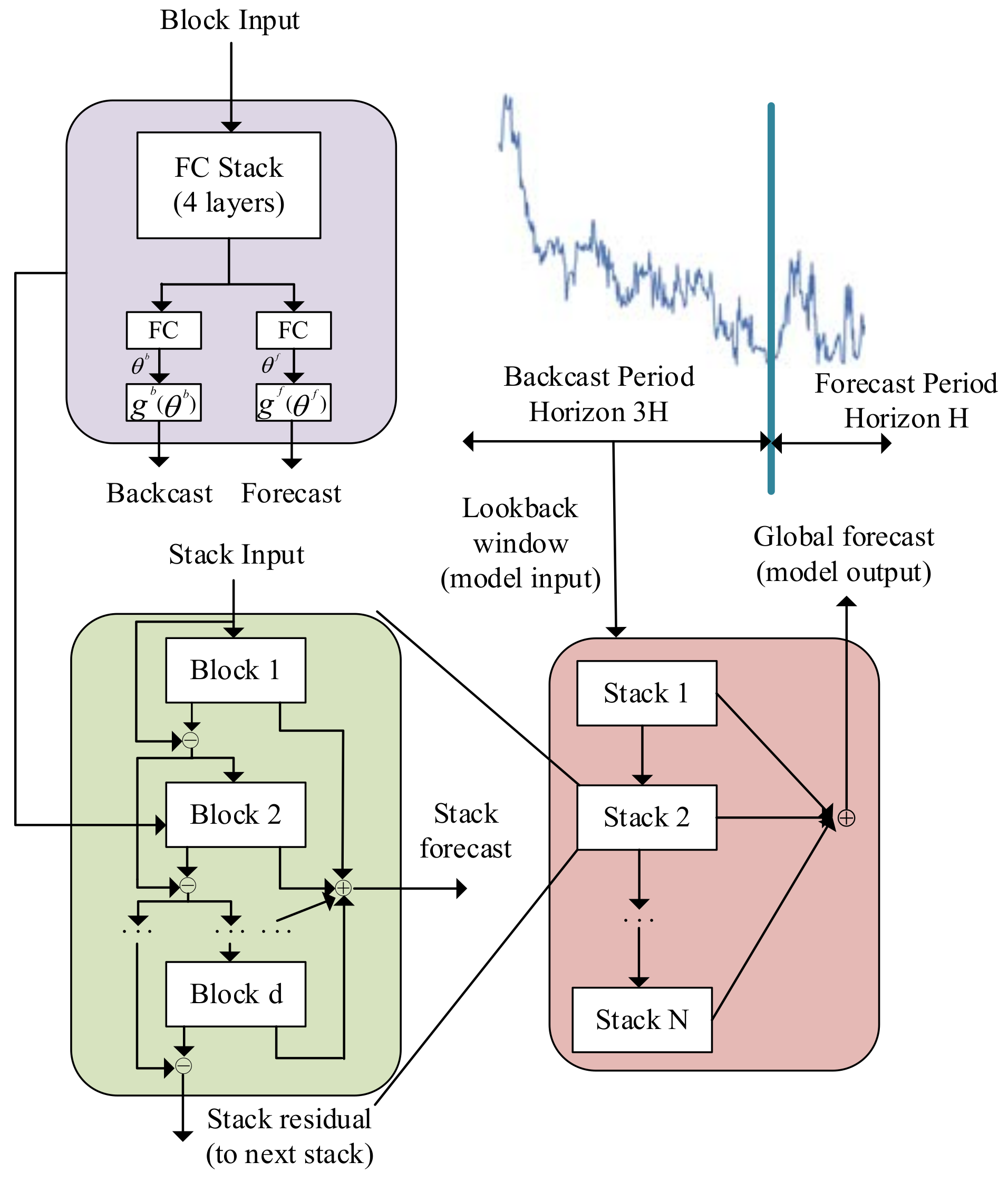
As shown in the top left part of Figure 2, the basic block is a multilayer FC network, consisting of two parts. The first part accepts the block input, then generates the forward output ${\theta }_f$ and the backward output ${\theta }_b$ for the next part. As the basis layer, the second part accepts the input from the first part, produces respective projections $g_f$ and ${\mathrm{g}}_b$, and outputs the forecast $\stackrel{\wedge }{{\mathrm{y}}_d}$ and the backcast $\stackrel{\wedge }{x_d}$ of the corresponding block d. The specific equations of the first part are as follows:

$${{\displaystyle h}}_{d,1}={{\displaystyle FC}}_{d,1}({{\displaystyle x}}_d),{{\displaystyle h}}_{d,2}={{\displaystyle FC}}_{d,2}({{\displaystyle h}}_{d,1}),{{\displaystyle h}}_{d,3}={{\displaystyle FC}}_{d,3}({{\displaystyle h}}_{d,2}),{{\displaystyle h}}_{d,4}={{\displaystyle FC}}_{d,4}({{\displaystyle h}}_{d,3})$$

(8)

$${{\displaystyle \theta }}_d^b={{\displaystyle LINEAR}}_d^b({{\displaystyle h}}_{d,4}),{{\displaystyle \theta }}_d^f={{\displaystyle LINEAR}}_d^f({{\displaystyle h}}_{d,4})$$

(9)

where $x_d$ is the block input, ${{\displaystyle FC}}_{d,i}$ represents the function of each layer of FC network, $i=1,2,3,4$, LINEAR is the linear function, ${{\displaystyle \theta }}_d^f={{\displaystyle W}}_d^f{{\displaystyle h}}_{d,4}$.

The specific equations of the second part are as follows:

$$\stackrel{\wedge }{y_d}=h_d^f\left({\theta }_d^f\right)$$

(10)

$$\stackrel{\wedge }{x_d}=h_d^b\left({\theta }_d^b\right)$$

(11)

where $h_d^f$ and $h_d^b$ are the function of ${\theta }_d^f$ and ${\theta }_d^b$, which can be set as a linear function or as a specific function. The details are shown in Equations (13) and (14).

• (2) Doubly residual stacking.

As shown in the lower left part of Figure 2, the hierarchical dual-residual topology has two residual branches. One branch accumulates the partial forecast ${\stackrel{\wedge }{y}}_d$ of each block to obtain the forecast output $\stackrel{\wedge }{y}$ of the corresponding stack. Another branch backcasts the input of each block, which makes the forecast of the next block easier. The specific equation is depicted as follows:

$$\left\{\begin{array}{l}{x}_d=x_{d-1}-{\stackrel{\wedge }{x}}_{d-1}\\ \stackrel{\wedge }{y}={\displaystyle \sum _d{\stackrel{\wedge }{y}}_d}\end{array}\right.$$

(12)

where $x_d$ and $x_{d-1}$ are the input of block d and block $d-1$, ${\stackrel{\wedge }{x}}_{d-1}$ is the backcast output of block $d-1$.

• (3) Interpretable architecture.

Oreshkin et al. [35] added the trend and seasonality model to increase the stack output’s interpretability. In the trend model, $h_d^f$ and $h_d^b$ are the linear function slowly varying:

$$\left\{\begin{array}{l}{\stackrel{\wedge }{y}}_{s,d}^{trend}=h_d^f\left({\theta }_{s,d}^f\right)={\displaystyle \sum _{\tau =0}^I{\theta }_{s,d,\tau }^f\times {\varphi }^{\tau }}\\ {\stackrel{\wedge }{x}}_{s,d}^{trend}=h_d^b\left({\theta }_{s,d}^b\right)={\displaystyle \sum _{\tau =0}^I{\theta }_{s,d,\tau }^b\times {\varphi }^{\tau }}\end{array}\right.$$

(13)

In the seasonality model, $h_d^f$ and $h_d^b$ are the periodic function of the Fourier series:

$$\left\{\begin{array}{l}{\stackrel{\wedge }{y}}_{s,d}^{seasonality}={\displaystyle \sum _{\tau =0}^{H/2-1}{\theta }_{s,d,\tau }^f\cos \left(2\pi \tau \varphi \right)}+{\theta }_{s,d,\tau +H/2}^f\sin \left(2\pi \tau \varphi \right)\\ {\stackrel{\wedge }{x}}_{s,d}^{seasonality}={\displaystyle \sum _{\tau =0}^{H/2-1}{\theta }_{s,d,\tau }^b\cos \left(2\pi \tau \varphi \right)}+{\theta }_{s,d,\tau +H/2}^b\sin \left(2\pi \tau \varphi \right)\end{array}\right.$$

(14)

where ${\theta }_{s,d,\tau }^f$ is the element $\tau$ of the output of the forecast branch of the dth block in the sth stack, ${\theta }_{s,d,\tau }^b$ is the element $\tau$ of the output of the backcast branch of the dth block in the sth stack, $I$ is usually set to a small value (e.g., 2 or 3), $\varphi ={[0,1,2,\cdots ,H-1]}^T/H$, $H$ is the frequency of the forecast or backcast.

2.3. Interval Forecasting of Coal Price Adopting Quantile Regression

Since the N-BEATS algorithm cannot achieve the interval forecasting of coal prices, this paper uses quantile regression for interval forecasting. The quantile loss is as follows:

$$\begin{array}{c}{L}_q\left(m,{\stackrel{\wedge }{m}}^q\right)=\left\{\begin{array}{ll}q(m-{\stackrel{\wedge }{m}}^q)& m-{\stackrel{\wedge }{m}}^q>0\\ 0& m-{\stackrel{\wedge }{m}}^q=0\\ (1-q)({\stackrel{\wedge }{m}}^q-m)& m-{\stackrel{\wedge }{m}}^q<0\end{array}\right.\end{array}$$

(15)

where, at the given quantile level of $q$, $m$ and ${\stackrel{\wedge }{m}}^q$ represent the actual value and the predicted value of coal price, respectively, $q\in \left(0,1\right)$, when $m-{\stackrel{\wedge }{m}}^q=0$, $L_q\left(m,{\stackrel{\wedge }{m}}^q\right)=0$ means that predicted and actual values match perfectly. Each forecasting value at one group specific quantile level $Q=\left(q_1,\dots ,q_m\right)$ is calculated by minimizing quantile loss. The function of the total quantile loss is the following:

$$\begin{array}{c}{L}_Q={\displaystyle {\displaystyle \sum }_{o=1}^m}{L}_{q_j}\left(m,{\stackrel{\wedge }{m}}^{q_0}\right)\end{array}$$

(16)

2.4. Significance Analysis of Covariates

Mean impact value (MIV) can assess the correlation of various variables in the Back Propagation Neural Network (BPNN) and is widely used to filter the variables in BPNN [36]. Its absolute magnitude reflects the extent to which the covariates have an impact on the dependent variable. Based on the trained VCNQM model, this paper selects coal prices as the dependent variable, as well as 15 covariates, and calculates the MIV of each covariate. Firstly, the training set is adaptively trained with the VCNQM model. Then, each covariate is increased by 10% and decreased by 10% to obtain two new training sets, which are simulated according to the fitting model. The mean of the difference between the two simulation results is calculated as the sample size, namely MIV. Ultimately, this paper sorts the covariates according to their absolute MIV and eliminates those with smaller effects to achieve attribute parsimony.

3. Empirical Study

3.1. Data Description

In this paper, we refer to the relevant literature on coal to establish the main indicator system of coal prices. Ultimately, we adopt the main indicator system of coal price from Wu et al. [29], which selected the drivers of coal price from energy, supply, demand, weather, international market, and macroeconomics.

The energy dimension included the New York natural gas spot price (NPNGSP), the Daqing oil spot price (DCOP), the wind power industry index (WPII), and the hydropower industry index (HII) [37,38]. The supply-and-demand dimension contained the coal mining industry index (CMII), the industrial index (II), and the A-share power industry index (ASESI). The macroeconomics dimension consisted of the coal industry index (CII), the A-share index (ASI), the USD/CNY exchange rate (U/C), the AUD/CNY exchange rate (A/C), the overnight Shanghai interbank offered rate (SHIBOR), and the six-month treasury bond yield (SMTY) [39,40]. The international market dimension was represented by the Newcastle power coal spot price (NPCSP) [41]. The weather dimension was represented by average maximum temperature (Tem) of major cities in China [29].

Concerning coal prices, we use the composite average price index of Bohai Rim Steam Coal (Q5500k). The Bohai Rim ports are the main force of coal transportation in China, and their coal prices can effectively reflect China’s coal price situation [42].

For the above variables, the data from 9 October 2013 to 9 June 2020 are selected as the training set, and the data from 10 June 2020 to 28 January 2022 are selected as the test set. After collecting all the data, this paper detects the outliers of all the variables with the help of a scatter plot and eliminates them, then finally replaces the missing data with the help of linear interpolation in the given time frame. The results of the correlation tests between the coal price and its drivers are shown in

Table 1. Results of the correlation test.

Drivers	Tem	CMII	II	ASESI	A/C
Correlation coefficients	−0.10 *	0.18 **	−0.03	−0.23 **	0.05
Drivers	U/C	SMTY	SHIBOR	CII	ASI
Correlation coefficients	0.18 **	0.05	0.14 **	0.18 **	0.04
Drivers	NPCSP	NYNGSP	DCOP	HII	WPII
Correlation coefficients	0.81 **	0.17 **	0.34 **	0.43 **	0.12 *

Note: We calculated Pearson correlation coefficients; * and ** indicate significant correlation at 5% and 1% significance levels, respectively.

: (1) Most drivers are significantly correlated with coal prices. (2) A few drivers do not have a significant linear relationship with coal prices and may have a non-linear correlation with coal prices.

3.2. Benchmark Model and Parameter Setting

In this paper, we select various benchmark models for a cross-comparison with the VCNQM model to see whether the VCNQM model has better predictive performance. First, we select N-BEATS for comparative analysis with random forest (RF); support vector machine (SVM), Convolutional Neural Network (CNN), LSTM, and RNN models, and the results verify that N-BEATS outperforms them in forecasting coal prices. Second, we compare the performance of N-BEATS with the CVNM model, confirming joint signal decomposition techniques can improve the prediction accuracy of prediction models.

Given that the configuration of the model hyperparameters will affect its forecasting outcomes of coal price, we adopt grid search to determine the optimal parameters for the hybrid model. The grid search method is essentially an exhaustive method, whose advantage is that it is a simple and intuitive way to find the best combination for a given hyperparameter space. By specifying a list of candidate values for the hyperparameters, the grid search performs an exhaustive search of all possible parameter combinations, as well as model training and evaluation for each set of parameters, and finally selects the combination of parameters with the best performance as the hyperparameters for the final model [43,44]. The results of the hybrid model’s parameter settings are obtained through the grid search as follows:

(1)

In the CSA-VMD model, the population size of CSA is 30 and T is 100; $N$ is in the range of [2, 10], and $\alpha$ is in the range of [1000, 10,000].

(2)

In N-BEATS, the maximum value of time steps for backcasting and forecasting are 10 and 7, respectively, and the learning rate is 0.002; the pieces of information processed per batch are 16, 32, 64; the numbers of stacks are 16, 32, 64, with the numbers of blocks per stack being 1, 2, 3, and 5, respectively; the numbers of neurons that make up each fully connected layer in each block of each stack are 32, 64, 128.

4. Results and Discussion

4.1. Results of Coal Price Decomposition Using the CSA-VMD

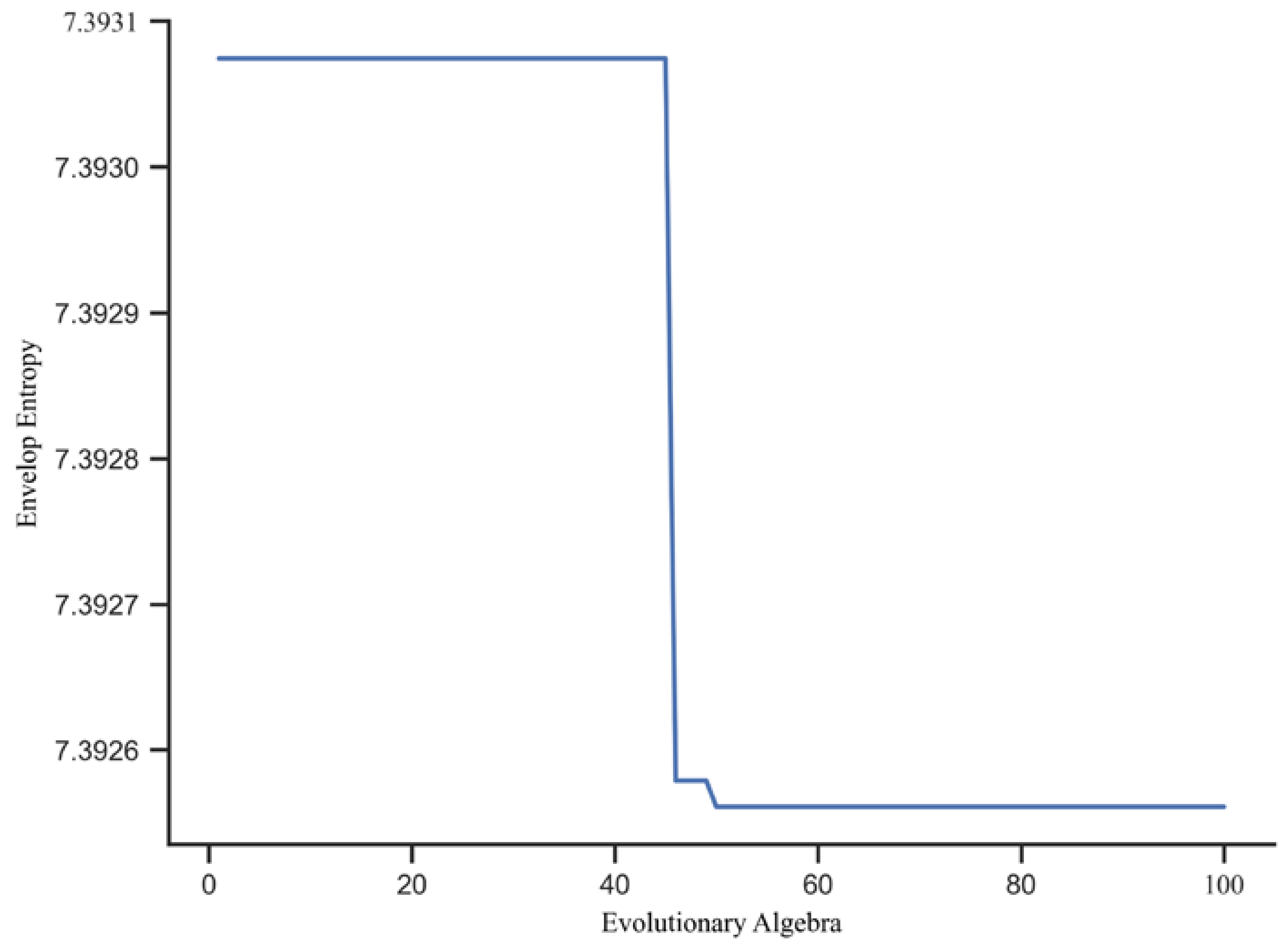
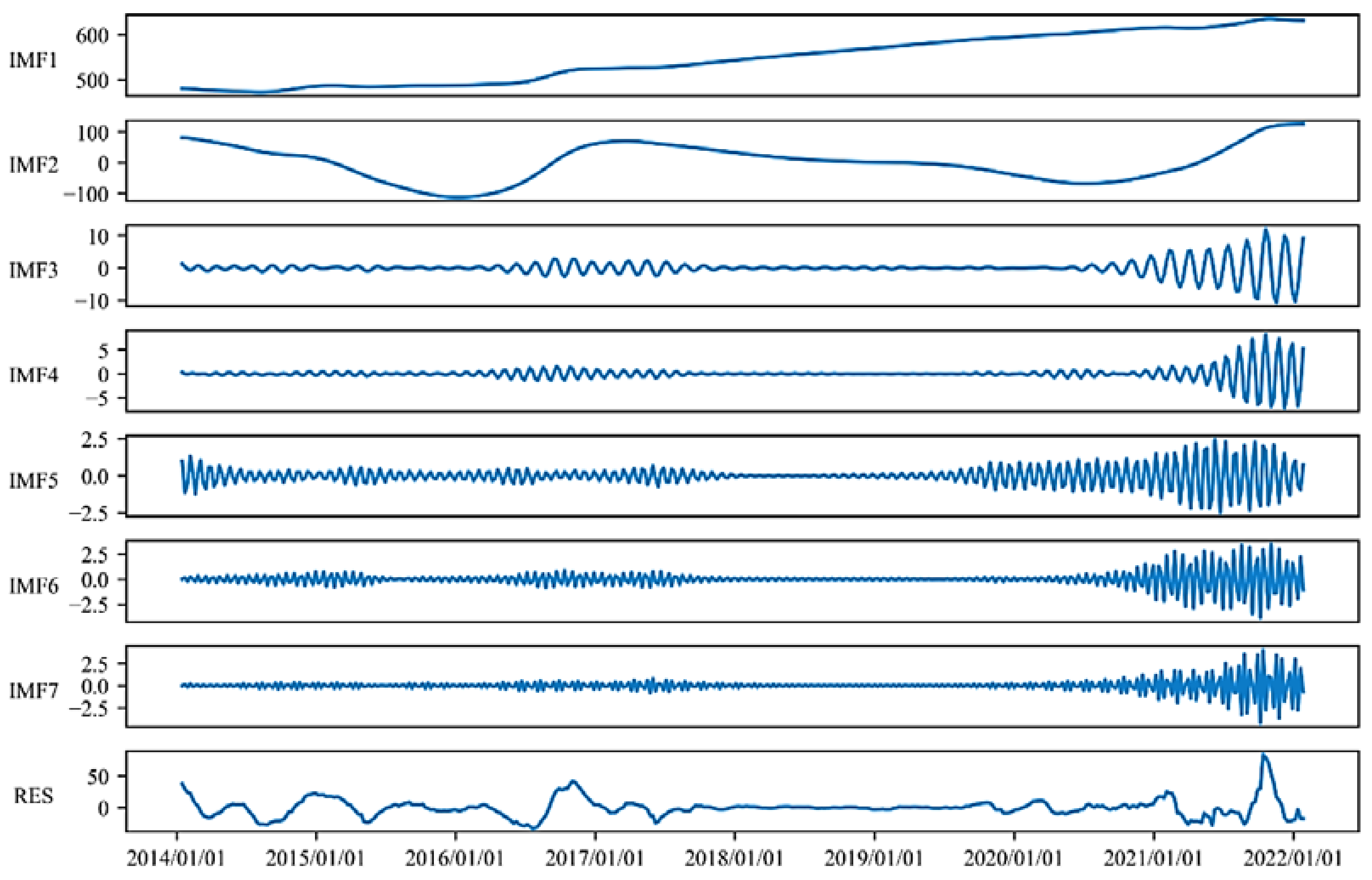
Although VMD is a workable method to decompose coal price sequences, its biggest challenge lies in finding the optimal parameters for the sequence decomposition. Therefore, we determine the optimal parameters of VMD by CSA-VMD, which avoids errors arising from the artificially selected parameters. By observing the statistical indicators in

Table 2. Statistical indicators of the weekly price of steam coal.

Steam coal weekly price	Observations	Max	Min	Average	Standard Deviation	Variance	Skewness	Kurtosis
	420	848	371	547.048	86.883	7548.580	0.076	1.110

and the trend of power coal prices in Figure 3, it can be concluded that the weekly price of steam coal displays obvious fluctuation changes, and its non-linear and non-stationary characteristics are considerable, in which the highest price is almost 1.3 times higher than the lowest, and the distribution is not near the mean most of the time, and its fluctuating tendency is neither linear nor obeys a normal distribution, making it challenging to identify its fluctuation trend pattern. As shown in Figure 4 and Figure 5, during the iteration of the CSA algorithm, the envelope entropy $E_A$ decreases to a minimum of 7.392561 at the 50th iteration, the corresponding quadratic penalty factor $\alpha$ is equal to 9864, and the corresponding decomposition modal number $N$ is equal to 7. The modal decomposition results of CSA-VMD in the above given parameter are shown in Figure 6. It shows that each modal component is relatively homogeneous with respect to the time domain. In comparison with the original weekly steam coal price series (seen in Figure 3), the decomposed subseries is less turbulent and its smoothness and linearity are more significant. Specifically, the fluctuations of the sub-signal IMF1 show a linearly increasing trend in the interval of [500, 600], and the fluctuations of the sub-signal IMF2 show a phased linear pattern in the interval [−100, 100]. Compared to the irregular fluctuations of original steam coal prices, both are more conducive to the identification and integration of subsequent N-beats models. The volatility of the sub-signals IMF3 and IMF4 also diminish, and despite a sharp increase in volatility in the last part of the time domain, the volatility interval is significantly narrower compared to the original coal price, with a low impact on the subsequent integration. Compared to IMF3 and IMF4, the fluctuations of the sub-signals IMF5, IMF6, and IMF7 are more and more obvious in the time domain, but their fluctuation intervals are further narrowed down, and the influence on the subsequent integration is negligible. Moreover, the smoothness of the sub-signals can be improved with the help of multiple decompositions, which is also the future direction for improvement in this paper.

4.2. Results of Point and Interval Forecasting Using the VCNQM Model

On the basis of the optimal parameters derived in the previous step, we achieve point forecasting of coal prices. Additionally, we construct the quantile loss function at the quantile of 0.50 of the forecasting value. The interval forecasting of coal price is also accomplished under the confidence level of 90%. For the sake of reflecting the forecasting effect of the VCNQM model visually, we make point and interval predictions of weekly coal prices with the hybrid model in the test set.

As displayed in Figure 7, the predictions of the VCNQM model are essentially near to coal price’s actual trend. Although the point forecasting result is excellent, the interval forecasting result is generally superior to the point forecasting. In the whole test set, the actual values basically fall within the prediction range of the interval forecasting, and the predicted interval coverage probability (PICP) is 0.9167, at a confidence level of 90%, certifying the validity of interval prediction results. In the decomposition stage, the subseries decomposed by CSA-VMD are more stable. In the integration phase, each stack of N-BEATS contains multiple blocks. After receiving and processing the input signal, each block produces a forecast output and a backcast output. The input of each block, minus its backcast output, is the input of the next block, which effectively improves the signal’s fitness. The forecast output of each stack is the integration of the forecast output of all blocks in that stack, and the forecast output of the whole network is the integration of the forecast output of all stacks in the network. Therefore, the VCNQM hybrid model has superior prediction performance.

4.3. Importance Analysis of Drivers

In the trained VCNQM model, different values of each driver are input in this paper to obtain their MIV corresponding to each covariate, which are taken as absolute values, leading to the following results.

Figure 8 illustrates the importance of each driver to coal prices, ordered by the absolute value of MIV from top to bottom. In particular, the A-share power industry index, with an MIV of 12.3566, has the greatest degree of influence on the price of coal in China, followed by the coal industry index, with an MIV of −7.2830. Then, there is the AUD/CNY exchange rate, the Daqing oil spot price, and the Newcastle power coal spot price in Australia, each with an MIV of −4.9466, 4.7000, and −4.6765, respectively. As a result, this paper concludes that the five factors mentioned above have a significant impact on coal prices, while the MIVs of the coal mining industry index and the overnight Shanghai interbank offered rate are 0.0710 and −0.2257, respectively, indicating the smallest degree of impact on coal prices and can therefore be ignored. Because most of China’s coal is used for thermal power generation, the A-share power industry index directly affects coal demand, which in turn affects coal prices. The coal industry index directly influences the supply of coal and thus the price of coal. Oil, as the main substitute for coal, has a direct impact on coal prices due to its price fluctuations. Since Australia was the primary supplier of China’s coal imports in the past, the AUD/CNY exchange rate and the Newcastle power coal spot price in Australia directly influenced China’s coal supply and thus domestic coal prices.

4.4. Comparison Analysis of Different Models’ Forecasting Performance

This paper excludes the decomposition part of the VCNQM model and compares the single model, namely N-BEATS, with the hybrid model to test the robustness of the hybrid model. Moreover, to verify that the VCNQM model has better prediction performance, we selected a variety of benchmark models for cross-comparison with the VCNQM model. Meanwhile, the mean absolute percentage error (MAPE), the mean absolute proportional error (MASE), the mean absolute error (MAE), and the symmetric mean absolute percentage error (SMAPE) are selected as metrics in this paper.

As shown in

Table 3. The ablation experiment of the VCNQM model.

Model	MAPE	MASE	MAE	SMAPE
N-Beats	11.49%	27.16	67.53	10.45%
VCNQM	11.33%	26.83	66.72	10.42%

, compared with N-BEATS, MAPE, MASE, MAE, and SMAPE of the VCNQM model are reduced by 0.16%, 0.33, 0.81, and 0.03%, respectively. This suggests that the hybrid model’s series decomposition procedure is capable of lowering the original signal’s volatility and enhancing its forecasting capabilities.

As shown in

Table 4. Performance metrics for different models.

Model	MAPE	MASE	MAE	SMAPE
RF	16.28%	43.04	89.73	15.97%
SVM	14.9%	42.11	86.51	14.75%
RNN	13.6%	31.45	78.19	12.47%
GRU	12.55%	29.10	72.67	11.89%
LSTM	12.37%	28.89	71.84	11.24%
N-Beats	11.49%	27.16	67.53	10.45%
VCNQM	11.33%	26.83	66.72	10.42%

, VCNQM exhibits better performance on all measures. Compared with the RF, the MAPE, MASE, MAE, and SMAPE of the VCNQM model are reduced by 4.95%, 16.21, 23.01, and 5.55%, respectively. Compared with the SVM, the MAPE, MASE, MAE, and SMAPE of the VCNQM model are reduced by 03.57%, 15.28, 19.79, and 4.33%, respectively. RF and SVM are to machine learning methods that are sensitive to noise and missing values, making it difficult for them to cope with highly volatile coal prices [45]. Compared to RNN, all the measures of VCNQM are also reduced by 2.27%, 4.62, 11.47, 2.05%. Compared to GRU, all the measures of VCNQM are also reduced by 1.22%, 2.27, 5.95, 1.47%. Compared with LSTM, the MAPE, MASE, MAE, and SMAPE of VCNQM are reduced by 1.04%, 2.06, 5.12, and 0.83%, respectively. GRU, LSTM and RNN mainly perform sequential processing over time, and training them requires a lot of information [46,47]. The decomposition part of the hybrid model, CSA-VMD, decomposes the coal price series into a number of smoother sub-sequences, which facilitates subsequent integration forecasting. The integration part of the hybrid model, N-BEATS, integrates all the sub-series forecasts to output a final coal price point forecast. N-BEATS enables parameter sharing to regularize the neural network and improve the generalization ability by learning multiple tasks at the same time. Therefore, compared to GRU, LSTM, and RNN, VCNQM is more weakly affected by the deficiency of information and outperforms them in forecasting coal prices.

5. Conclusions

To implement accurate forecasting of coal prices in China, we developed a unique decomposition integration forecasting model and applied a hybrid frequency data set containing multiple drivers for empirical analysis. The results verify that the VCNQM hybrid model possesses more excellent forecasting capability and a wider application scope compared to a single model. Based on the above research, we come to the following conclusions:

(1)

CSA-VMD as the decomposition method can effectively improve the stationarity and linearity of the coal price series. Specifically, the CSA-VMD model enhances not only the rationality of parameter determination but also the decomposition accuracy, but also decomposes the coal price signal into multiple sub-signals with weaker volatility.

(2)

Quantile regression can perform the interval forecasting for coal prices and extends the breadth of application of the VCNQM hybrid model.

(3)

The A-share power industry index and the coal industry index are the most important drivers of China’s steam coal price. They all directly or indirectly have an impact on coal supply and thus coal prices.

(4)

In comparison with previous deep neural networks, the VCNQM hybrid model exhibits superior prediction performance, with remarkably lower errors. Excluding the decomposition part of the hybrid model, the predictive performance of the single model N-BEATS is worse than that of the hybrid model.

5.1. Literature Contributions

The decomposition integration hybrid model is a popular method for coal price prediction in academic areas. During the decomposition stage, Wei [18], Wu, and Huang [19], as well as Torres et al. [20], found that the signal decomposition results of EMD and its variants suffer from modal confusion and pseudo-modes. In addition, a new decomposition method called ICEEMDAN, proposed by Niu et al. [21], is only conducive to long-term forecasting. Although Rayi et al. [23] and Li et al. [24] demonstrated that VMD makes up for the deficiencies of EMD and its variants, the decomposition parameters of VMD need to be chosen artificially, which affects the decomposition accuracy and causes boundary effects. Therefore, for the sake of raising the accuracy and rationality of signal decomposition, we adopted envelope entropy as the fitness function and used CSA to iteratively update the parameters until the optimal parameters were generated.

During the integration stage, Zhang et al. [25] and Niu et al. [21] used LSTM and GRU to integrate subseries, respectively. Their final outputs lacked interpretability, which is not conducive for decision-makers to make sense of the model’s prediction results or identify potential pitfalls. In addition, to raise the extensibility of the application of the forecasting model, Ding et al. [30] used kernel density estimation for coal price interval forecasting, which is influenced by the width of the subintervals. Therefore, in this paper, we applied N-BEATS and quantile regression to realize interval forecasting, which effectively avoided the aforementioned problems.

5.2. Management Insights

Based on the above findings, we produce the following management insights:

(1)

To control coal prices, the government can realize this goal by controlling coal mining, adjusting coal imports, and developing relevant power industry policies.

(2)

To timely respond to the drastic volatility of the coal market, relevant enterprises should always pay attention to the information related to the power industry, coal mining and domestic coal imports, and make corresponding assessments and adjustments of future coal prices according to their changes.

5.3. Future Prospects

In response to this paper, we can also consider the following enhancements in our future research:

(1)

Adding multiple decompositions to the hybrid model may be more effective in weakening the fluctuation of the coal price series and increasing its predictive effectiveness.

(2)

Incorporating more factors into the coal price driver system, such as relevant policies, environmental quality, etc.

(3)

Investigating other interval prediction methods to accomplish better prediction results.

References

1. Wang, C.; Xu, G.; Sun, C.; Xu, J.; Xu, K.; Jiang, L.; Wang, Y.; Su, S.; Hu, S.; Xiang, J. Modeling and forecasting of coal price based on influencing factors and time series. J. Clean. Prod. 2024, 467, 143030. [Google Scholar] [CrossRef]
2. Pan, W.; Guo, Z.; Zhang, J.S.Y.; Luo, L. Forecasting of coal and electricity prices in China: Evidence from the quantum bee colony-support vector regression neural network. Energy Econ. 2024, 134, 107565. [Google Scholar] [CrossRef]
3. Kostecka-Jurczyk, D.; Struś, M.; Marak, K. The Role of Energy Cooperatives in Ensuring the Energy and Economic Security of Polish Municipalities. Energies 2024, 17, 3082. [Google Scholar] [CrossRef]
4. Gajdzik, B.; Wolniak, R.; Nagaj, R.; Zuromskaite-Nagaj, B.; Grebski, W.W. The influence of the global energy crisis on energy efficiency: A comprehensive analysis. Energies 2024, 17, 947. [Google Scholar] [CrossRef]
5. Ferrari, D.; Ravazzolo, F.; Vespignani, J. Forecasting energy commodity prices: A large global dataset sparse approach. Energy Econ. 2021, 98, 105268. [Google Scholar] [CrossRef]
6. Guo, X.; Shi, J.; Ren, D. Coal price forecasting and structural analysis in China. Discret. Dyn. Nat. Soc. 2016, 7, 1236168. [Google Scholar] [CrossRef]
7. Jiang, S.; Yang, C.; Guo, J.; Ding, Z. ARIMA forecasting of China’s coal consumption, price and investment by 2030. Energy Sources Part B Econ. Plan. Policy 2018, 13, 190–195. [Google Scholar] [CrossRef]
8. Zhao, Z.Y.; Zhu, J.; Xia, B. Multi-fractal fluctuation features of thermal power coal price in China. Energy 2016, 117, 10–18. [Google Scholar] [CrossRef]
9. Herrera, G.P.; Constantino, M.; Tabak, B.M.; Pistori, H.; Su, J.J.; Naranpanawa, A. Long-term forecast of energy commodities price using machine learning. Energy 2019, 179, 214–221. [Google Scholar] [CrossRef]
10. Bonita, O.; Muflikhah, L. Comparison of Gaussian and ANOVA Kernel in Support Vector Regression for Predicting Coal Price. In Proceedings of the 2018 International Conference on Sustainable Information Engineering and Technology (SIET), Malang, Indonesia, 10–12 November 2018; pp. 147–150. [Google Scholar] [CrossRef]
11. Fan, X.; Wang, L.; Li, S. Predicting chaotic coal prices using a multi-layer perceptron network model. Resour. Policy 2016, 50, 86–92. [Google Scholar] [CrossRef]
12. Matyjaszek, M.; Fernández, P.R.; Krzemień, A.; Wodarski, K.; Valverde, G.F. Forecasting coking coal prices by means of ARIMA models and neural networks, considering the transgenic time series theory. Resour. Policy 2019, 61, 283–292. [Google Scholar] [CrossRef]
13. Chen, X.; Yu, R.; Ullah, S.; Wu, D.; Li, Z.; Li, Q.; Qi, H.; Liu, J.; Liu, M.; Zhang, Y. A novel loss function of deep learning in wind speed forecasting. Energy 2022, 238, 121808. [Google Scholar] [CrossRef]
14. Yeh, H.H.; Sun, M.T. Coal price prediction using financial indices. In Proceedings of the 2019 International Conference on Technologies and Applications of Artificial Intelligence (TAAI), Kaohsiung, Taiwan, 21–23 November 2019; pp. 1–6. [Google Scholar] [CrossRef]
15. Wang, H.; Ye, J.; Huang, L.; Wang, Q.; Zhang, H. A multivariable hybrid prediction model of offshore wind power based on multi-stage optimization and reconstruction prediction. Energy 2023, 262, 125428. [Google Scholar] [CrossRef]
16. Alameer, Z.; Fathalla, A.; Li, K.; Ye, H.; Jianhua, Z. Multistep-ahead forecasting of coal prices using a hybrid deep learning model. Resour. Policy 2020, 65, 101588. [Google Scholar] [CrossRef]
17. Wang, B.; Wang, J. Energy futures prices forecasting by novel DPFWR neural network and DS-CID evaluation. Neurocomputing 2019, 338, 1–15. [Google Scholar] [CrossRef]
18. Wei, L.Y. A hybrid ANFIS model based on empirical mode decomposition for stock time series forecasting. Appl. Soft Comput. 2016, 42, 368–376. [Google Scholar] [CrossRef]
19. Wu, Z.; Huang, N.E. Ensemble empirical mode decomposition: A noise-assisted data analysis method. Adv. Adapt. Data Anal. 2009, 1, 1–41. [Google Scholar] [CrossRef]
20. Torres, M.E.; Colominas, M.A.; Schlotthauer, G.; Flandrin, P. A complete ensemble empirical mode decomposition with adaptive noise. In Proceedings of the 2011 IEEE International Conference on Acoustics, Speech and Signal Processing (ICASSP), Prague, Czech Republic, 22–27 May 2011; pp. 4144–4147. [Google Scholar] [CrossRef]
21. Niu, H.; Xu, K.; Liu, C. A decomposition-ensemble model with regrouping method and attention-based gated recurrent unit network for energy price prediction. Energy 2021, 231, 120941. [Google Scholar] [CrossRef]
22. Wang, P.; Tao, Z.; Liu, J.; Chen, H. Improving the forecasting accuracy of interval-valued carbon price from a novel multi-scale framework with outliers detection: An improved interval-valued time series analysis mode. Energy Econ. 2023, 118, 106502. [Google Scholar] [CrossRef]
23. Rayi, V.K.; Mishra, S.P.; Naik, J.; Dash, P.K. Adaptive VMD based optimized deep learning mixed kernel ELM autoencoder for single and multistep wind power forecasting. Energy 2022, 244, 122585. [Google Scholar] [CrossRef]
24. Li, H.; Chang, J.; Xu, F.; Liu, Z.; Yang, Z.; Zhang, L.; Zhang, S.; Mao, R.; Du, X.; Liu, B. Efficient lidar signal denoising algorithm using variational mode decomposition combined with a whale optimization algorithm. Remote Sens. 2019, 11, 126. [Google Scholar] [CrossRef]
25. Zhang, K.; Cao, H.; Thé, J.; Yu, H. A hybrid model for multi-step coal price forecasting using decomposition technique and deep learning algorithms. Appl. Energy 2022, 306, 118011. [Google Scholar] [CrossRef]
26. Zhang, S.; Luo, J.; Wang, S.; Liu, F. Oil price forecasting: A hybrid GRU neural network based on decomposition–reconstruction methods. Expert Syst. Appl. 2023, 218, 119617. [Google Scholar] [CrossRef]
27. Fang, Y.; Wang, W.; Wu, P.; Zhao, Y. A sentiment-enhanced hybrid model for crude oil price forecasting. Expert Syst. Appl. 2023, 215, 119329. [Google Scholar] [CrossRef]
28. Li, R.; Song, X. A multi-scale model with feature recognition for the use of energy futures price forecasting. Expert Syst. Appl. 2023, 211, 118622. [Google Scholar] [CrossRef]
29. Wu, S.; Xia, G.; Liu, L. A novel decomposition integration model for power coal price forecasting. Resour. Policy 2023, 80, 103259. [Google Scholar] [CrossRef]
30. Ding, L.; Zhao, Z.; Han, M. Probability density forecasts for steam coal prices in China: The role of high-frequency factors. Energy 2021, 220, 119758. [Google Scholar] [CrossRef]
31. Mirjalili, S.; Gandomi, A.H.; Mirjalili, S.Z.; Saremi, S.; Faris, H.; Mirjalili, S.M. Salp swarm algorithm: A bio-inspired optimizer for engineering design problems. Adv. Eng. Softw. 2017, 114, 163–191. [Google Scholar] [CrossRef]
32. Braik, M.S. Chameleon swarm algorithm: A bioinspired optimizer for solving engineering design problems. Expert Syst. Appl. 2021, 174, 114685. [Google Scholar] [CrossRef]
33. Kin, G.O.; Challu, C.; Marcjasz, G.; Weron, R.; Dubrawski, A. Neural basis expansion analysis with exogenous variables: Forecasting electricity prices with NBEATSx. Int. J. Forecast. 2023, 39, 884–900. [Google Scholar] [CrossRef]
34. Dragomiretskiy, K.; Zosso, D. Variational mode decomposition. IEEE Trans. Signal Process 2014, 62, 531–544. [Google Scholar] [CrossRef]
35. Oreshkin, B.N.; Carpov, D.; Chapados, N.; Carpov, D. N-BEATS: Neural basis expansion analysis for interpretable time series forecasting. arXiv 2019, 1905, 10437. [Google Scholar] [CrossRef]
36. Zheng, G.; Li, K.; Yue, X.; Zhang, Y. A multifactor hybrid model for carbon price interval prediction based on decomposition-integration framework. J. Environ. Manag. 2024, 363, 121273. [Google Scholar] [CrossRef]
37. Filimonova, I.V.; Nemov, V.Y.; Komarova, A.V.; Mishenin, M.V.; Kozhevin, V.D. Relationship of renewable energy consumption to economic, environmental and institutional factors in Europe. Energy Rep. 2021, 7, 358–365. [Google Scholar] [CrossRef]
38. Li, R.; Leung, G.C. The relationship between energy prices, economic growth and renewable energy consumption: Evidence from Europe. Energy Rep. 2021, 7, 1712–1719. [Google Scholar] [CrossRef]
39. Batten, J.A.; Brzeszczynski, J.; Ciner, C.; Lau, M.C.; Lucey, B.; Yarovaya, L. Price and volatility spillovers across the international steam coal market. Energy Econ. 2019, 77, 119–138. [Google Scholar] [CrossRef]
40. Chandrarin, G.; Sohag, K.; Cahyaningsih, D.S.; Yuniawan, D.; Herdhayinta, H. The response of exchange rate to coal price, palm oil price, and inflation in Indonesia: Tail dependence analysis. Resour. Policy 2022, 77, 102750. [Google Scholar] [CrossRef]
41. Lin, B.; Chen, Y. Dynamic linkages and spillover effects between CET market, coal market and stock market of new energy companies: A case of Beijing CET market in China. Energy 2019, 172, 1198–1210. [Google Scholar] [CrossRef]
42. Gu, F.; Wang, J.; Guo, J.; Fan, Y. How the supply and demand of steam coal affect the investment in clean energy industry? Evidence from China. Resour. Policy 2020, 69, 101788. [Google Scholar] [CrossRef]
43. Nevendra, M.; Singh, P. Empirical investigation of hyperparameter optimization for software defect count prediction. Expert Syst. Appl. 2022, 191, 116217. [Google Scholar] [CrossRef]
44. Gao, R.; Liu, J.; Zhou, Q.; Duru, O.; Yuen, K.F. Newbuilding ship price forecasting by parsimonious intelligent model search engine. Expert Syst. Appl. 2022, 201, 117119. [Google Scholar] [CrossRef]
45. Sundaram, A.; Alkhaldi, N.S. Multi-Objective Stochastic Paint Optimizer for Solving Dynamic Economic Emission Dispatch with Transmission Loss Prediction Using Random Forest Machine Learning Model. Energies 2024, 17, 860. [Google Scholar] [CrossRef]
46. Acharya, S.K.; Yu, H.; Wi, Y.M.; Lee, J. Multihousehold Load Forecasting Based on a Convolutional Neural Network Using Moment Information and Data Augmentation. Energies 2024, 17, 902. [Google Scholar] [CrossRef]
47. Wang, F.; Lin, H.; Ma, Z. Transmission Line Icing Prediction Based on Dynamic Time Warping and Conductor Operating Parameters. Energies 2024, 17, 945. [Google Scholar] [CrossRef]
Figure 1. General structure of the hybrid model.
Energies 17 04166 g001
Figure 2. Framework of N-BEATS.
Energies 17 04166 g002
Figure 3. Weekly steam coal prices.
Energies 17 04166 g003
Figure 4. Envelope entropy.
Energies 17 04166 g004
Figure 5. As the number of iterations proceeds, the parameter optimization process of the VMD becomes more refined. (a) Quadratic penalty factor; (b) Number of decomposition modes.
Energies 17 04166 g005
Figure 6. Modal decomposition results of CSA-VMD.
Energies 17 04166 g006
Figure 7. Point and interval forecasting based on VCNQM. Note: the blue shaded area depicts the interval forecasting of coal price at a confidence level of 90%.
Energies 17 04166 g007
Figure 8. Absolute value of MIV for each driver. Note: see Section 3.1 for symbol descriptions.
Energies 17 04166 g008