Article

The Impact Time Series Selected Characteristics on the Fuel Demand Forecasting Effectiveness Based on Autoregressive Models and Markov Chains

Faculty of Civil Engineering, Cracow University of Technology, 31-155 Krakow, Poland
*
Author to whom correspondence should be addressed.
Energies 2024, 17(16), 4163; https://doi.org/10.3390/en17164163
Submission received: 17 June 2024 / Revised: 14 August 2024 / Accepted: 16 August 2024 / Published: 21 August 2024
(This article belongs to the Section G: Energy and Buildings)

Abstract

:
This article examines the influence of specific time series attributes on the efficacy of fuel demand forecasting. By utilising autoregressive models and Markov chains, the research aims to determine the impact of these attributes on the effectiveness of specific models. The study also proposes modifications to these models to enhance their performance in the context of the fuel industry’s unique fuel distribution. The research involves a comprehensive analysis, including identifying the impact of volatility, seasonality, trends, and sudden shocks within time series data on the suitability and accuracy of forecasting methods. The paper utilises ARIMA, SARIMA, and Markov chain models to assess their ability to integrate diverse time series features, improve forecast precision, and facilitate strategic logistical planning. The findings suggest that recognising and leveraging these time series characteristics can significantly enhance the management of fuel supplies, leading to reduced operational costs and environmental impacts.

1. Introduction

Predicting future customer demand has always been a challenge for supply chain systems. Accurately predicting future needs allows supply chain experts to plan and execute operational strategies more effectively. Such forecasting helps determine the quantity of products for each retailer, ideal stock levels, production and shipping amounts from manufacturing plants, and projected raw material purchases for upcoming months. In an environment characterised by globalisation, swift technological advancements, and heightened consumer expectations, firms within the same supply chain must collaborate to outperform rivals [1]. Demand prediction is foundational for planning and sourcing strategies, enhancing the supply chain’s agility and efficiency [2]. Thus, refining demand prediction techniques has grown increasingly vital for producers, suppliers, and sellers [3,4]. It is no different for the fuel sector, where effective forecasting of fuel demand can be crucial to achieving a company’s competitive advantage in the market. Forecasting this demand is not merely essential for ensuring operational fluidity but also stands as paramount for a broad spectrum of decision-making processes that influence the entire supply chain in the fuel industry. Accurate demand forecasting at fuel stations is not just a vital component for inventory level optimisation but also an indispensable tool in the planning and management of fuel transportation. Efficient delivery planning, based on precise forecasts, can yield significant cost savings and enhance operational efficiency. Anticipating higher demand at specific times allows companies to organise transport more cost-effectively. Accurate forecasts allow rapid response to unforeseen changes in demand, enabling transport plans to be adjusted to current needs. It helps prevent costly supply interruptions, which can result in customer loss and impact brand image and ensures the fleet’s effective utilisation, reducing transportation costs and CO2 emissions. The publication [5] presents how demand forecasting influences decisions regarding warehouse locations and delivery route planning. The document highlights that dynamic demand forecasting can affect logistical decisions and allow for rapid adaptation to changing market conditions. The forecasts that were obtained enabled the updating of transport routes using MILP models and dynamic programming, resulting in a significant reduction in the total distance travelled by vehicles and, consequently, the energy consumed and CO2 emissions. In the works [6,7], a detailed literature review concerning the green vehicle routing problem (GVRP) was conducted. These studies emphasise the importance of integrating environmental aspects, including energy efficiency, into logistical planning processes. The authors point out various methods and techniques that can be used to solve the GVRP, suggesting that precise demand forecasting is fundamental for the effective implementation of green routes. The research underscores that effective demand forecasting allows for better adaptation of routes and delivery methods to changing conditions. This enables companies to adjust their logistical infrastructure to actual demand, minimising inefficient resource utilisation and maximising energy savings. These effects are even more pronounced when fuel distribution to stations is implemented under the VMI (Vendor Management Inventory) concept, which is when the supplier controls the amount of fuel delivered and can shape inventory levels throughout the fuel network it serves. However, forecasting fuel demand at stations is exceptionally intricate due to the dynamics and irregularities of demand, making it difficult to predict through conventional methods. In this context, time series characteristics play a pivotal role. Volatility, seasonality, trends, or sudden shocks—all these features can influence the choice of an appropriate forecasting method. As not every method is suitable for every type of data, understanding and identifying these time series’ properties is critical to selecting the most apt forecasting model that ensures maximum forecast accuracy. In this article, we scrutinise forecasting methods based on ARIMA, SARIMA, and Markov chain models, considering their ability to account for specific time series characteristics.
This study aims to initially test the assumption that an adequate forecasting method can be identified based on the characteristics of a time series. To achieve this goal, the study examined the impact of selected time series characteristics on predictive accuracy for various forecasting models that model fuel demand. This research focuses on determining the impact of specific time series features on the effectiveness of specific models and how these models can be adjusted or improved to better utilise these features in the context of the fuel industry’s specific fuel distribution. In addition, the study considers the implications of these results for supply chain management in the fuel industry. In a practical context, the optimal use of forecasting methods can significantly contribute to improving planning processes at gas stations, enabling companies to plan the purchase and distribution of fuel accurately. Consequently, this can increase operational efficiency, translating into cost reductions and reduced CO2 emissions. Our aim is not only to identify the most effective forecasting techniques in the fuel industry context but also to understand how different time series features impact the efficiency of these methods. Hence, the intermediate goal of the study is to verify which model—ARIMA, SARIMA, or Markov chain—does the best job of integrating these specific time series characteristics into demand forecasts.
The rest of the paper is organised as follows: in Section 2, a brief literature review on demand forecasting methods was carried out, and Section 3 presents the basics of forecasting with ARIMA/SARIMA models and Markov chains. Section 4 presents the assumptions for the study and describes a numerical example based on actual fuel demand data at selected petrol stations in Poland. Section 5 presents the study’s results, the forecasting error values, and the correlation analysis of the considered time series characteristics with the performance measures for the different forecasting methods. The last section contains conclusions, recommendations, and a summary of the survey.

2. Brief Literature Review on Demand Forecasting Methods

The increasing ease of data collection, access to ever-growing amounts of data, and changing consumer trends mean that demand forecasting becomes an even more complex task despite the availability of many tools and literature sources. Over the past decades, the literature has seen numerous studies on various demand forecasting methods in different engineering and economics fields. Current methods can be divided into two groups: traditional techniques founded on mathematical models and those rooted in artificial intelligence [8]. The former encompasses methods like linear regression, moving average, weighted average, exponential smoothing, and other statistical approaches. Methods of causal analysis, like regression and econometrics, are employed to identify the determinants of demand and assess their influence on future demand patterns. Such a methodology is beneficial in comprehending the root causes of demand fluctuations and forecasting how alterations in these determinants might impact future demand [9]. Time series analysis methods like Autoregressive Moving Average (ARIMA) and its seasonal counterpart (SARIMA) are frequently employed for sales and demand forecasting [8]. As the research findings presented in publications show, these methods achieve suitable results in forecasting demand in various areas, including the retail industry and the fuel and energy sectors [10,11]. Few studies propose the use of Markov chains for modelling and demand forecasting. In [12], the author proposed Markov chain models for forecasting return flows in the supply chain. Meanwhile, Ref. [13] presents the use of Markov chains in forecasting demand in urban bike-sharing systems. Markov chains can also be successfully used in forecasting financial markets [14]. In contrast, Ref. [15] presents a literature review of hidden Markov chains’ applications in various engineering areas. Meanwhile, researchers’ interest in artificial intelligence-based sales and demand forecasting methods has risen. This category involves expert systems, fuzzy logic, neural networks, and hybrid systems integrating multiple AI approaches. Among these, the neural network model is particularly popular, with many studies highlighting its advantages over traditional models, mainly due to its adaptability. In the domain of supervised and deep learning, scientific work focuses on different methods. The most prevalent techniques include Multi-Layer Perceptron (MLP), Long Short-Term Memory (LSTM), and Artificial Neural Network (ANN). When it comes to conventional ML techniques, there’s a marked preference for supervised learning approaches [16,17]. There is also no shortage of studies in which the authors focus on examining the effectiveness of both statistical forecasting and AI methods to match the proper method for a given type of product. Falatouri [18] explored demand prediction in the retail supply chain using time series methodologies. They then created SARIMA and LSTM models. Their findings indicated that the LSTM model was superior for stable demand, while SARIMA was more effective for seasonally influenced products. Additionally, when they factored in the influence of advertising using the SARIMAX model, they found that SARIMAX was best suited for products influenced by advertising campaigns. In [19], a thorough literature review can be found on applying machine learning and artificial intelligence methods in demand forecasting. The authors point to a growing number of studies combining several methods to increase forecasting accuracy. Increasingly, there are studies in which forecasting methods based on artificial intelligence are combined with optimisation methods to enhance the efficiency of forecasting models. In [20], the authors tested LSTM models with hidden neurons in different LSTM layers, and particle swarm metaheuristics optimised the number of epochs in the learning process. Despite numerous studies on demand forecasting, the issue of forecasting fuel demand is still not sufficiently explored [21]. In [10], the authors conducted a literature review, which indicates that, so far, few studies have addressed the forecasting of fuel demand at gas stations.
Few works still address the problem of investigating how selected time series characteristics, such as variance, seasonality, type of probability distribution, autocorrelation, etc., can affect forecasting performance and the appropriate choice of methods. In [22], the authors introduce the concept of similarity between series. They used various clustering techniques to identify similar series groups and then created a forecasting model based on the LSTM. In [23], a visualisation method for time series collections was proposed, which allows for representing a time series as a point in a two-dimensional instance space based on selected characteristics (spectral entropy, strength of trend, strength of seasonality, seasonal period, first-order autocorrelation, optimal Box–Cox transformation parameter). The study evaluated the effectiveness of selected forecasting methods for the group of examined time series. Authors demonstrated that certain forecasting techniques performed better in specific areas of the time series feature space than others. In [24], a subjective and algorithmic method for selecting a forecasting model based on time series features was examined. As a result, they proposed a combination of these methods, achieving suitable results. Qin [25] studied the effect of time series length on the quality of ARIMA forecasting models.

3. Fuel Demand Prediction Based on ARIMA and Markov Chains Models

3.1. Basics of Forecasting with Markov Chains

Markov chains are relatively simple and powerful tools that allow for the modelling of processes where future states depend solely on the current state, not on how that state was achieved. In the case of a gas station, this means that the demand on a given day or hour primarily depends on the demand from the previous day or hour, not on the sales history from weeks or months ago. One can account for cyclical changes in demand through the appropriate state structure in a Markov chain, such as spikes during weekends, holidays, or other periods. Unlike more complex forecasting methods, like neural networks, Markov chains are relatively easy to understand and interpret, which can be a key to gaining acceptance and trust from gas station employees. The key to modelling with Markov chains is defining “states” and the transition probabilities between these states. If hidden patterns in the data can be represented as states and transitions between them, Markov chains can effectively detect and model them.
Markov’s process is a sequence of random variables in which the probability of what will happen depends only on the present state. In the considered issue, only Markov processes defined on a discrete space of states (Markov chains) will be used.
Let us denote by X = X 0 ,   X 1 ,   , X t , , X t m a x a sequence of discrete random variables. The value of the variable   X t will be called the state of the chain s k at the moment t. The finite set of states can be defined as state space S as follows:
s S , S = s 1 , s 2 , , s k 1 , s k , k <
It is assumed that the set of states S is calculable. The discrete timestamps used in the considered problem can be defined as follows:
t T , T = 1,2 , , t m a x , t m a x
Definition 1.
A sequence of random variables X is a Markov chain if the Markov condition is fulfilled:
P X t + 1 = s t + 1     X t = s t , X t 1 = s t 1 , , X 0 = s 0 =                   = P X t + 1 = s     X t = s t      t T   s 0 ,   , s t , s t + 1 S
Thus, for the Markov chain, the distribution of the conditional probability of position in the time step t depends only on the conditional probability of position in the previous step and not on previous trajectory points (history).
Definition 2.
Let  P  be a matrix of dimensions (k × k) and elements p i j : i , j = 1 , k . A sequence of random variables X 0 ,   X 1 ,    with values from a finite set of states, S = s 1 ,   s 2 , , s k 1 ,     s k  is called the Markov process with the transition matrix P , if for each t , and any i , j { 1 , k } and all states:
P = p i j = P X t + 1 = s j     X t = s i
The probability p i j is the conditional probability that represents the chance that state s i at step t will change to state s j at the next time step t + 1 . The elements of the transition matrix p i j fulfil the following conditions:
t T : p i j = P X t + 1 = s j     X t = s i
p i j 0 i , j { 1 , k }
i : j { 1 , k } p i j = 1
Definition 3.
The Markov chain is homogeneous when, for each time stamp, it is described by the same transition matrix script  P . The transition matrix is fixed and does not depend on time.
In the use of Markov chains, the initial state plays a crucial role. Formally, the initial state is a random variable X 0 . Therefore, the Markov chain often starts with a certain probability distribution across the state’s space.
Definition 4.
The initial distribution  π 0 ( s i )  is a vector defined as follows:
π 0 ( s i ) = π 0 s 1 , π 0 s 2 ,   , π 0 s k = P { X 0 = s i : s i S }  
To determine the distribution of the forecasted state of the modelled object for one time step ahead, the following equation can be used:
π t + 1 = π t + 1 · P
Note that the π t + 1 or π t are the row vectors; thus, we have the following:
π 1 = π 0 · P π 2 = π 1 · P = π 0 · P 2 π 3 = π 2 · P = π 0 · P 3
π t + 1 = π 0 · P t + 1
For simplicity, the probability transitions do not change over time in most Markov chain applications. These models are called homogeneous Markov chains (HMCs). However, the assumption of stationarity is not justified in the case of human-created demand, where the demand for fuels exhibits significantly different behaviour at different times (e.g., different seasons) and in different phases of cycles [26]. For this reason, heterogeneous Markov chains, where the transition matrix is time-varying, were used in the subsequent analysis. Despite lacking a classical stationary distribution, heterogeneous Markov chains (similarly known as non-homogeneous Markov chains) are effectively used in forecasting, especially in contexts where conditions change dynamically over time. Several methods and applications have been described in the scientific literature that may be useful in practice [26,27].

3.2. Basics of Forecasting with SARIMA/ARIMA Models

ARIMA models are based on the autocorrelation phenomenon, which means the correlation of variable values forecasted with the values of the same variable is delayed in time. The main characteristic feature of ARIMA models is that the value of the predicted variable at time t is a linear combination of values of the same variable from previous periods t 1 ,   t 2 ,   . . . ,   t p increased by a certain value of the random component. Among such models, we can distinguish three basic types:
  • Autoregressive models (AR);
  • Moving average models (MA);
  • Mixed autoregressive and moving average models (ARMA).
In a general way, the autoregressive model of order p can be represented as follows:
Y t = φ 0 + φ 1 Y t 1 + φ 2 Y t 2 + + φ p Y t p + e t
where
  • Y t ,   Y t 1 ,   Y t 2 ,   Y t p —the value of the variable, respectively, at the time t ,   t 1 ,   t 2 ,   t p ;
  • φ 0 ,   φ 1 ,   φ 2 ,   φ p —model parameters;
  • e t —value of random component at the period t ;
  • p —order lag.
Delay parameter p determines how far back in time we should reach to determine the value of the forecasted variable at time t . If the random components of the past are correlated, we have to deal with the process of moving average (MA), which is expressed by the following formula:
Y t = ϑ 0 ϑ 1 e t 1 ϑ 2 e t 2 ϑ q e t q + e t
where
  • e t , e t 1 , e t 2 , e t q —residuals of the model, respectively, at the period t ,   t 1 ,   t 2 ,   t q ;
  • ϑ 0 , ϑ 1 , ϑ 2 , ϑ q —model parameters;
  • q —order lag.
The connection of (AR) and (MA) parts of the model is often made to better adapt the model to the historical data. It is known as the ARMA model, which has both p and q parameters. This combination may be represented as follows:
Y t = φ 0 + φ 1 Y t 1 + φ 2 Y t 2 + + φ p Y t p + e t ϑ 0 ϑ 1 e t 1 ϑ 2 e t 2 ϑ q e t q
SARIMA (Seasonal Autoregressive Integrated Moving Average) is an extension of the ARIMA (Autoregressive Integrated Moving Average) model that incorporates seasonality in addition to the non-seasonal components. The SARIMA model is defined as SARIMA ( p ,   d ,   q ) ( P ,   D ,   Q ,   s ) , where p is the number of seasonal AR terms, D is the number of seasonal differences, Q is the number of seasonal MA terms, and s is the seasonal period.
The SARIMA model can be formulated as follows:
X t * = c + φ 1 X t 1 * + φ 2 X t 2 * + + φ p X t p * + ϑ 1 e t 1 + ϑ 2 e t 2 + ϑ q e t q + Φ 1 X t s * + + + Φ P X t P s * + Θ 1 e t s + + Θ Q e t Q s
where
  • X t * is the differentiated value of the time series at time t , obtained after taking d differences for the general and D differences for the seasonal component;
  • φ 1 , φ 2 ,… are the parameters of the autoregressive model;
  • ϑ 1 , ϑ 2 ,… are the parameters of the moving average model;
  • Φ 1 , Φ 1 ,… are the parameters of the seasonal autoregressive model;
  • Θ 1 , Θ 2 ,… are the parameters of the seasonal moving average model.
SARIMA models perform well with time series and seasonal patterns, which is a frequently observed characteristic when forecasting fuel demand at gas stations.

4. Assumptions and Research Methodology Description

4.1. Methodology Framework

The models used in the study, such as ARIMA, SARIMA, and Markov chain, are widely used because they can model and predict complex patterns in time series data. Each method has specific assumptions that can affect its effectiveness in different contexts.
The ARIMA method assumes that the time series is stationary or has been transformed to stationary form, meaning that its statistics, such as mean and variance, do not change over time. A limitation of this method is its inability to model series with distinct seasonal patterns without additional modifications, such as seasonal differentiation in SARIMA models. The SARIMA model, an extension of ARIMA, adds the ability to model seasonality in the data, which is crucial in the case of fuel demand, which exhibits distinct seasonal patterns. However, both ARIMA and SARIMA can be limited when dealing with data with irregular peaks or sudden changes, which are not well modelled by the linear approach of these methods.
Classical Markov chains are characterised by a transparent structure, making understanding the mechanisms governing demand variability easier. With the ability to model in the form of states and transitions between them, Markov chains can effectively capture the dynamics of demand that change over time in response to external factors like price changes, seasonality, or special events. In fuel demand modelling, where consumer behaviour can exhibit strong temporal dependencies (e.g., demand spikes on certain days of the week or hours), Markov chains effectively account for these dependencies through probabilistic mechanisms. As a probabilistic method, Markov chains are particularly useful in scenarios with high uncertainty and variability in the data. Markov chains offer a framework for modelling this uncertainty in the context of fuel demand, where external factors can significantly affect demand.
As was mentioned in Section 3.1, our approach uses a time-updated transition matrix between states to enable the construction of more precise forecasts. In this way, the model is “taught” with the latest data and trends. As a result, forecasts can better reflect real changes in demand, which is especially important in rapidly changing market conditions. There is no homogeneity requirement in the literature on time series forecasting using Markov chains, and the use of heterogeneous models is often more justified due to changing conditions [13]. For example, publications [14,27] examine Markov chains with a time-varying transition matrix, i.e., heterogeneous. The authors reason that a time-varying transition matrix better reflects reality, where conditions change dynamically. This allows greater flexibility than static, homogeneous models assuming unchanging transition probabilities.
The methodology adopted for the research includes four phases: input data phase, models construction phase, forecasting phase, and correlation analysis phase. The methodology used is shown in Figure 1. The first phase involved selecting a representative time series representing daily fuel demand based on data from a telemetric measurement system. The system monitors the filling level of the fuel tank at the station. The selected data were analysed for consistency and validity. The following individual characteristics were determined for each series in the set under consideration: standard deviation, power spectral density, dominant periodic component, Hurst exponent, and first lag value of the autocorrelation function. Each parameter characterises different aspects of the data, allowing a better understanding of its structure and potential relationships. The standard deviation and power spectral density help to understand the variability of the data and their energy distribution at different frequencies, which helps select methods capable of handling series with clear cycles and trends. The dominant periodic component indicates significant cycles in the data, suggesting the effectiveness of methods that account for seasonality, such as SARIMA or seasonal decomposition methods. The Hurst exponent was chosen because of its ability to examine long-term relationships in the data. Meanwhile, the value of the first lag of the autocorrelation function may indicate the effectiveness of simple autoregressive (AR) models.
The ARIMA, SARIMA, and Markov chain forecasting models were developed individually for each time series in the model-construction phase. Details on the implementation of the individual models are contained in Section 4.2. The predicted fuel demand values for one day ahead were determined in the forecasting phase. To adapt the models to the time-varying dynamics of a given time series, a rolling data window was used in the analysis, allowing the parameters of the autoregressive models ARIMA, SARIMA, and the transition matrix for Markov chains to be updated with each latest demand observation. A 30-day empirical forecast verification period was used to verify the accuracy of the forecasts. Based on this, the average values of MAPE and RMSE errors were determined for each series. In the final phase of the study, which was a correlation analysis, it was examined which of the considered individual characteristics and features of a particular time series might influence the magnitude of the MAPE error achieved for each of the methods under consideration. The analysis aims to verify two issues: first, whether the selected series characteristics are suitable indicators describing the series, and second, whether an adequate forecasting method can be selected based on the series characteristics. The analysis that is conducted, to some extent, can help solve the problem of choosing the appropriate forecasting method for a specific time series with certain features. This issue is becoming increasingly important from the perspective of enterprises collecting ever-larger data sets, aiming to use them in decision-making processes.
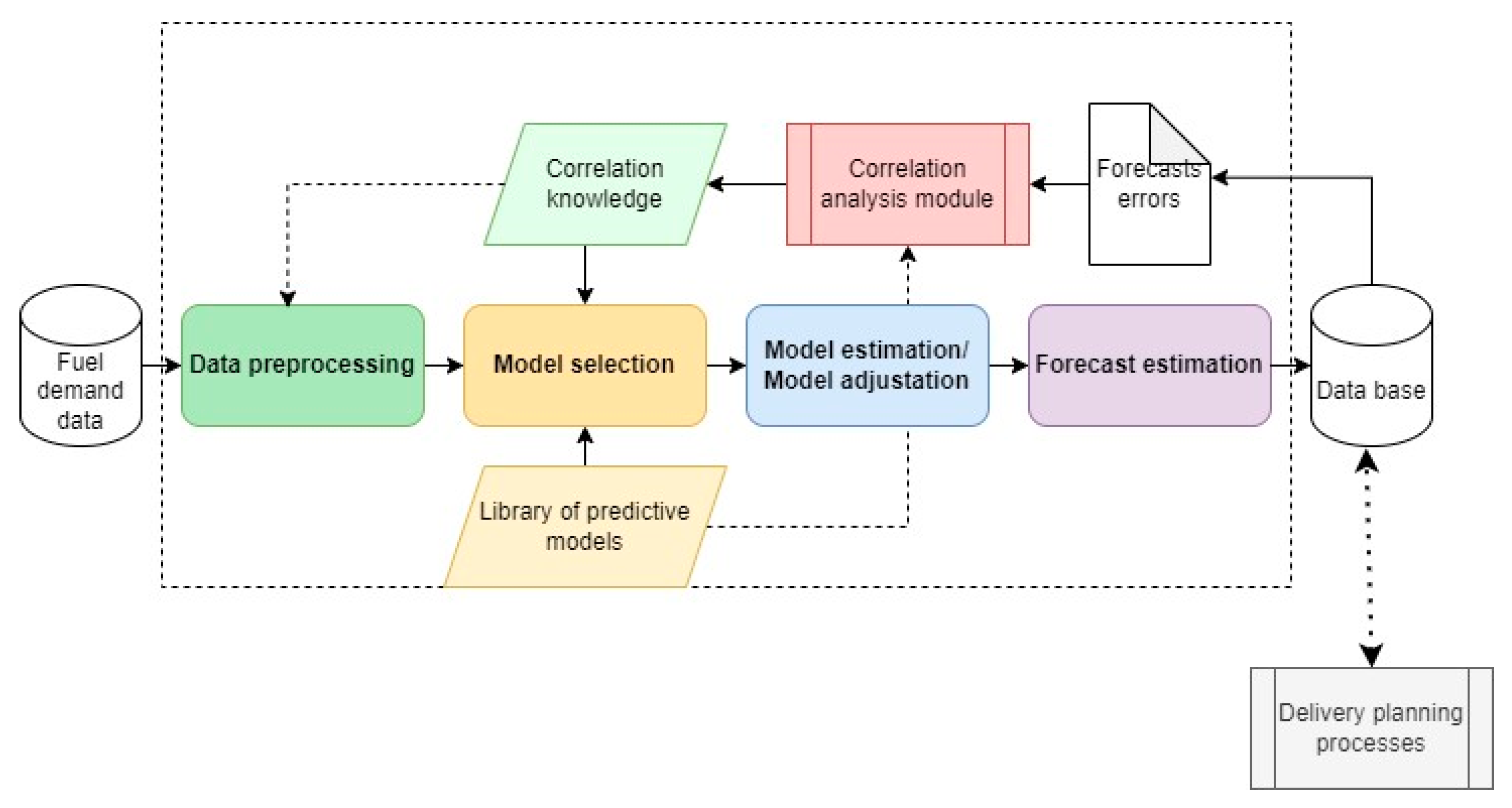
In the case of implementing the knowledge resulting from such an analysis in the actual information systems of an enterprise, a forecasting module can be created, which will adaptively select the appropriate model. An example conceptual model of such a module is presented in Figure 2.
In the discussed framework, we commence with the data concerning fuel consumption at various outlets. By utilising distinct characteristics of a particular time series, which are delineated in the “Correlation Knowledge” base, one can perform estimations through “Data preprocessing.” This “Correlation Knowledge” base comprises a compilation of guidelines and rules delineated and refined via the methodology expounded in this study. Possessing a repertoire of forecasting techniques (“Library of predictive models”) alongside a suite of indicators and time series traits, one can discern the interconnections among these framework components within the “Correlation analysis module.” Leveraging this insight enables the identification of an optimal predictive model (“Model selection”) that promises minimal forecast error. Under the presumption that this conceptual schema operates as a perpetual cycle, subsequent phases involve either calibrating the parameters of the chosen forecast model or refining an existing model (Model estimation/Model adjustment). If shifts in demand dynamics are substantial, there may be a need to overhaul the model’s structural parameters and the entire forecast model type. Following such an adjustment, the forecast for a predetermined planning interval can be computed using the rejuvenated model. These projections are instrumental in orchestrating fuel supply logistics to service stations. The cycle then proceeds to gather actual demand data, evaluate the precision of forecasts, and continuously refine the understanding of how time series attributes correlate with forecast accuracy. This model ensures adaptability and accounts for the fluctuating nature of demand patterns, facilitating the derivation of highly accurate forecasts while conserving computational resources. While the proposed schematic is designed with LPG demand forecasting in mind, its application is not limited to this domain alone. The paper preliminarily validates this framework by integrating ARIMA and SARIMA models, as well as Markov chains within the “Library of Predictive Models” and specific indicators within the “Correlation Knowledge.” Meanwhile, the “Correlation analysis module” is confined to traditional correlation coefficient assessments, though alternative methodologies, including machine learning tools, could be employed provided a sufficiently large dataset is available.

4.2. Data

Data were collected regarding the daily sales volume for 85 gas stations from 1 May 2018 to 3 July 2022 to conduct research. A characteristic feature of the demand for gaseous fuels is the variability and randomness of the occurrence of values. Figure 3 presents a histogram for the coefficient of variation for the entire data survey sample (the coefficient of variation was calculated as the quotient of the standard deviation and the mean value). As can be seen, only 35 of the 85 series have a variability of up to 27%; the other 50 have a much higher variability, of which 18 have a high variability of more than 50%.
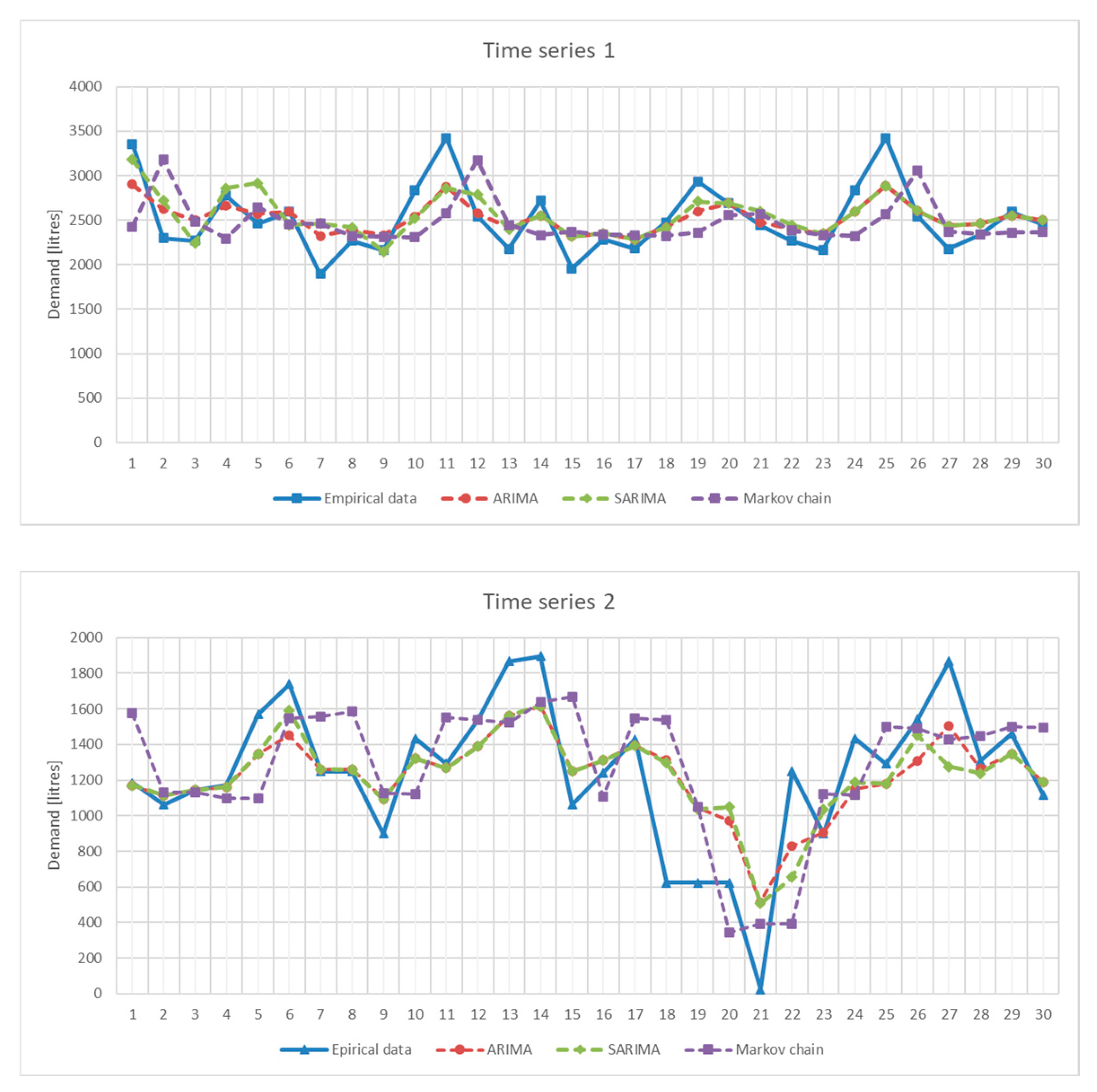
Figure 4 presents two time series demonstrating the variability of fuel demand at two selected stations for the last 180 time series values.
The dataset was divided into two parts: a learning and verification set. The verification set comprised the last 30 values of each time series, while the learning set comprised the remaining values. The data from the verification set were used to assess the quality of the forecast. In contrast, the methodology adopted assumes a rolling window of analysis and the realisation of the forecast one step ahead. This means that successive time series values from the verification set were iteratively added to the learning set, and in each iteration, new forecasting models were developed after a new value was added, as described below.

4.3. Assumptions for Forecasting Models Development

4.3.1. ARIMA/SARIMA Models

Main assumptions for developing ARIMA and SARIMA models: The model was trained on the last 180 historical values from the learning set (a more extended series does not provide significant information for forecasting, and a shorter period was characterised by more significant forecast inaccuracy). Each time series was analysed using a rolling window approach, meaning that the training data were used to develop a forecasting model for the first day of the verification period. Forecasts for subsequent days in the verification period were made iteratively with new ARIMA and SARIMA models (in terms of updating parameter values and estimating structural parameters) by adding a new value from the verification period to the training set while maintaining a constant number of observations equal to 180. For each time series, 30 models from the ARIMA and SARIMA groups were developed for each forecasted value in the verification period.
Each series was tested with the KPSS test (Kwiatkowski–Phillips–Schmidt–Shin unit root test) to determine the stationarity of the series. Based on this test, the parameter’s value related to the degree of series integration in the ARIMA model was selected. Assuming the rolling window approach for developing forecasting models, the KPSS test was also re-evaluated each time. As a result, in some cases, the time series alternated between stationary and non-stationary, even though the data described demand at a specific station. This phenomenon specifically affected 24 stations, where shifting the window and replacing the oldest values with new, current ones caused the KPSS test to yield different results. For 30 stations, despite the window shifting, the series exhibited non-stationarity, while for 21 stations, the series remained stationary.
For SARIMA models, the seasonality period was determined using power spectral density analysis. The cyclical component with the highest degree of explanation of the series variance was selected for the models. The model’s other non-seasonal components (p, d, q) were selected based on tests of different model configurations. The upper limit of the model parameters ( p m a x , d m a x , q m a x ) was determined separately for each series based on the analysis of the autocorrelation ACF and partial autocorrelation PACF function. In the next step, various model configurations were iteratively checked, from the simplest types (1, 1, 1) to more complex ones, whose non-seasonal parameter values were determined in the previous step. An appropriate model was selected by minimising the AIC (Akaike Information Criterion), i.e., the model was chosen for which the AIC value was the smallest.

4.3.2. Markov Chain Models

In a real system, the data describing a stochastic process such as demand are discrete but continuous observations, i.e., there is the possibility of sudden changes. This evolutionary nature of the data may not correctly correspond to the assumptions of homogeneous Markov chains. When the variation has an insignificant stochastic contribution, it is usual to extract from the set of measurements the distribution described by the formula (10). By observing the process again at a future time t + τ and counting the number of observed transitions between states, a transition matrix P τ can be defined that satisfies the following conditions:
π t + τ = π t · P τ
The matrix
P τ = p τ ,    i , j i , j S
is called the transition matrix at time τ :   τ [ 1 , , n ] , where n is number of a forecast horizon. In the case under consideration, referring to the verification set, the planning horizon is 30, hence τ [ 1 , , 30 ] .
In the case of non-homogeneous Markov chains, the Markov property is preserved, but the transition probability may depend on time [14]. Heterogeneous Markov chains are particularly useful in short-term forecasting, where we know the transition matrix for subsequent time steps in advance. In this case, we can track the evolution of the probability distribution for subsequent states by taking into account the change in the transition matrix P τ at each time step. Short-term forecasting does not require the existence of a stationary distribution, as it focuses on predicting states in the next few time steps. More theoretical considerations on the assumptions of non-homogeneous Markov chains can be found in [28,29], among others.
Analogous to the ARIMA and SARIMA models, in the case under consideration, the variable transition matrix was estimated each time for a new data window (rolling analysis window for data from the verification set) individually for each time series set. Transition matrices were estimated when a new demand value from the verification set was added to the set T , after which a new state forecast value was calculated, which was converted into a point forecast according to the approach described below.
To implement Markov chains for forecasting purposes, it is necessary to appropriately define the state space for each series. The number of states for the analysed time series was determined analogously to the method of determining the number of classes in histogram construction. Thus, each state represents a specific range of demand values with a width of X w (for the sake of readability, we have omitted the index linked to the consecutive number of the time series, the formula being applied for each time series separately):
X w = max X m i n ( X ) N
where
  • max X , m i n ( X ) —respectively, the maximum and minimum value of the time series X ;
  • N —the number of observations in the time series X .
The formula is based on the idea that the width of the interval should be proportional to the range of the data divided by the square root of the number of observations, leading to smaller interval widths for larger data sets, which can be useful in certain contexts. However, this is a less standard approach compared to the aforementioned rules. The rationale behind this assumption is that fuel demand can be highly variable, resulting in many potential states with zero or very low probability of occurrence.
The method of assigning specific demand value ranges to specific state numbers from the state space S = s 1 , s 2 , , s k 1 ,   s k   is illustrated in Figure 5.
Conventionally, from Equation (9), the forecasted state distribution π t + 1 is obtained. To obtain the point forecasted demand value, it was determined as follows:
If π t + 1 = π t + 1 s 1 , π t + 1 s 2 , , π t + 1 s k describes the probability of a given state occurring in the forecast horizon t + 1, then the point value of the forecasted demand Y t + 1 P   was determined as follows:
Y t + 1 P = j = 1 k π t + 1 s j · X ^ j
where
  • π t + 1 s j —probability value for the forecasted state s j of the time series;
  • X ^ j —the midpoint of the demand interval assigned to the j -th state in the time series.
The above formula assumes that the forecasted point demand value is determined as the sum of the products of the forecasted state probabilities and the corresponding value representing the midpoint of the demand interval assigned to the state s j . In this way, for all time series, all forecasts were obtained for each period.

5. Numerical Experiment Results

5.1. Forecast Accuracy Analysis

Forecast accuracy was analysed for all 85 time series considered. The mean absolute percentage error (MAPE) and the root mean square error (RMSE) were used to assess the effectiveness of the developed models. Accuracy measures were calculated for each observation in the 30-day verification period. Then, the average value of the indicators was determined for each series. Example forecast results for the selected two time series for the verification period are presented in Figure 6. The Markov chain method yielded better results for these selected two series than the ARIMA or SARIMA models. For example, for time series 1, the MAPE error was 8.7% for the Markov chain forecasting method, for the ARIMA models, it was 12.7%, and for the SARIMA model, the error was 14.8%. However, throughout the sample, there were time series for which the Markov chains yielded worse results than the ARIMA or SARIMA models.
The obtained values were used to analyse the distribution of error values in the entire examined time series set. Figure 7 presents the distribution of the average percentage errors (MAPEs) across the entire set of analysed data. The range of the “box” from Q1 (first quartile) to Q3 (third quartile) is called the interquartile range and represents the middle 50% of the data. In the considered case, the “whiskers” extend from the box to values that are 1.5 times the interquartile range due to the presence of outliers, which are marked on the chart with red markers.
The results show that the Markov chain models were characterised by the smallest range of the MAPE percentage error in the entire series set compared to the other considered methods. ARIMA models, although achieving a minimum error value significantly lower than Markov chains, for one of the series, the average error level exceeded 70%, which was about ten percentage points worse than the maximum obtained by Markov chains. SARIMA models performed the worst in the presented set, achieving very high outlier values, reaching even 120%. The medians, minimum, and maximum error values for the entire dataset are presented in Table 1.

5.2. Influence of Time Series Characteristics on Forecast Accuracy

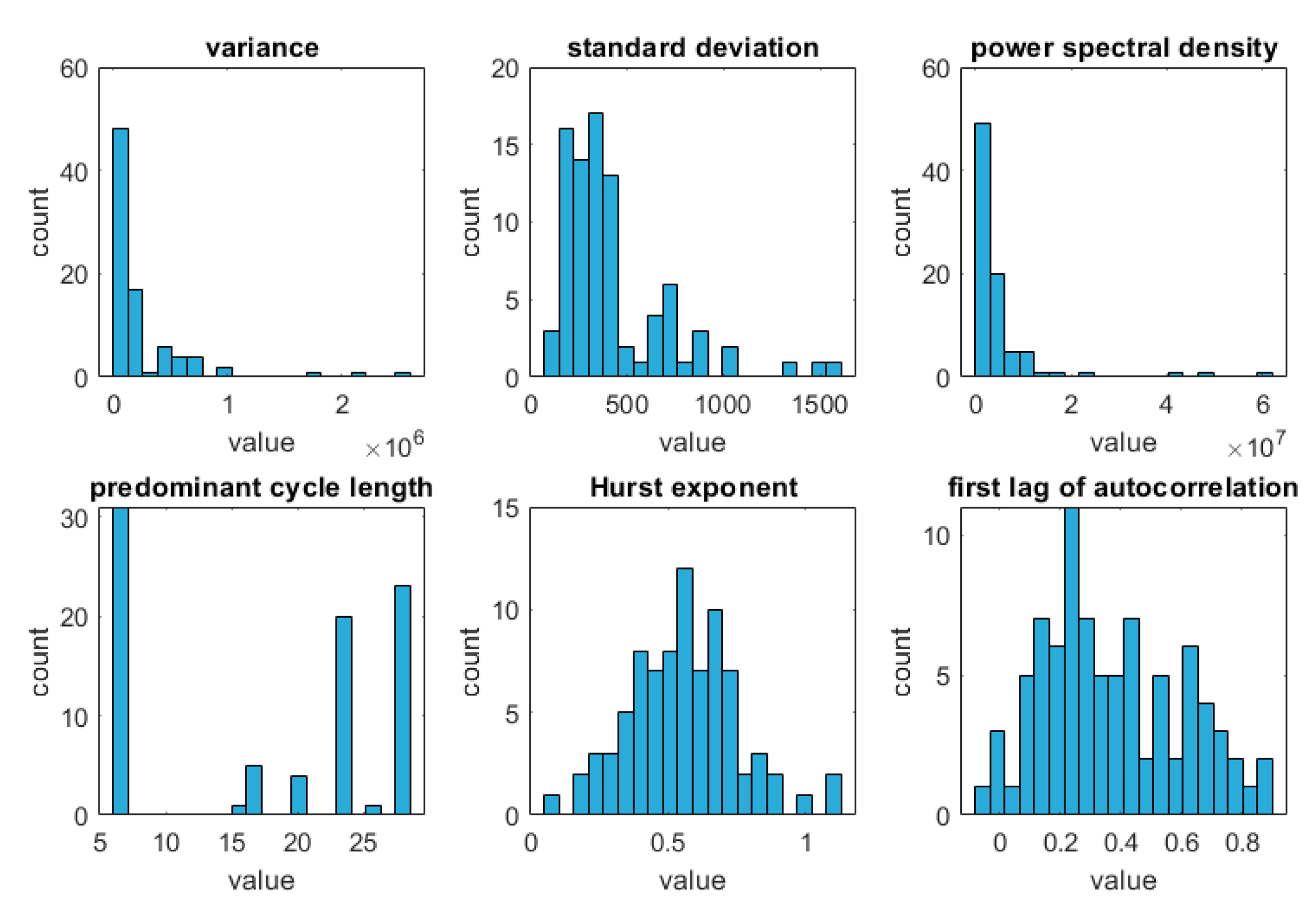
The results obtained in Section 5.1 naturally lead to the question of which characteristics of time series and to what extent can affect the size of the forecasting error achieved by a given forecasting method. Providing a partial answer to this question would enable the rational selection of a forecasting method for a specific time series with specific features. This would significantly limit the computational effort and the number of tests performed in practical applications to choose the appropriate forecasting approach. In the study, the values of six selected features that may affect the size of the forecasting error were determined for each time series. For this purpose, the following were calculated: variance, standard deviation, spectral power density, dominant length of the cyclical component, Hurst exponent, and the value of the first delay for the autocorrelation function ACF. Selected characteristics, besides providing information about the variability of the time series, also provide insight into how the variance of the time series is distributed to frequency, allowing for the identification of cyclical data patterns and the determination of dominant frequency components. The value of the first delay for the autocorrelation function can provide information about temporal dependencies in the series, which helps choose autocorrelation-based methods. Meanwhile, the Hurst exponent measures the long-term memory of the series; values close to one indicate greater predictability of the series. The distribution of examined feature values in the set of analysed series is presented in Figure 8.
In the analysed set of time series, the dominant cases have a standard deviation of 430 litres, which gives an average variation coefficient of 38%. Considering the length of the dominant periodic component, series with cycles of lengths 7, 18, 24, and 28 days prevail. For the Hurst exponent, 50% of cases have values between 0.4 and 0.6. Values around 0.5 indicate a time series close to a random series, making it difficult to predict. A total of 50% of the time series have first lag autocorrelation function values in the range between 0.2 and 0.5, indicating a moderate, positive temporal dependence between the observations of the time series. This means that the values of the time series are only to some extent predictable based on their previous values.
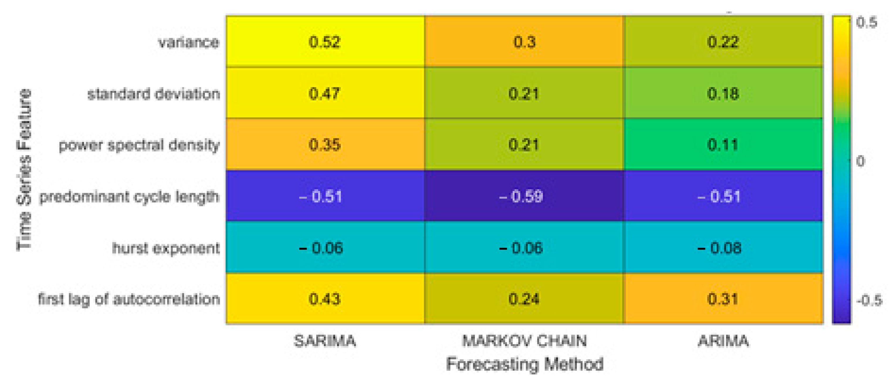
To determine the impact of individual characteristics on the MAPE forecasting error level, correlation coefficient values were calculated for each series characteristic in the entire dataset being considered. The obtained values are presented in Figure 9.
A Student’s t-test was used to assess the significance of this correlation coefficient. The null hypothesis is that there is no correlation in the sample. The critical value of t was read from the Student’s t-distribution table for a significance level of α = 0.05 and the corresponding number of degrees of freedom. If the calculated t-value is greater than the critical value of t α / 2 t (for a two-sided test), we reject the null hypothesis, meaning that the correlation coefficient is statistically significant. In the case analysed, all correlation coefficients for the Hurst exponent and the correlation coefficients between the MAPE errors for ARIMA and Markov chains, as well as the standard deviation and power spectral density, were found to be insignificant. The remaining correlation coefficients were statistically significant at the α = 0.05 .
Based on the obtained results, it can be pointed out that SARIMA models proved to be the most sensitive to error for series with high variance and standard deviation. Markov chains models and ARIMA models achieved decidedly lower correlation values (but values are not statistically significant). Markov chain models proved to be the most effective in recognising longer periodic cycles present in the series, where data variability is spread over a larger time range, facilitating the identification and forecasting of patterns. In this case, the correlation coefficient value was −0.59, indicating a moderate negative dependency strength. A weak positive dependency occurs in the case of correlation with the first delay value for the ACF function. Intuitively, it might seem that an increase in the first delay value of the autocorrelation function should result in a reduction in the forecasting error, as it suggests that observations are strongly correlated with each other over time, which theoretically should facilitate forecasting. However, several explanations for the situation were observed. If significant dependencies occur at greater delays and are omitted, this can lead to more significant forecasting errors. Additionally, suppose other factors and variables not included in the model influence the time series. In that case, this can also lead to more significant errors despite higher values of the first delay of the ACF function. No dependency was observed for the Hurst exponent values.

6. Conclusions

This article presents a study regarding the analysis of the impact of selected characteristics of time series on the effectiveness of forecasting fuel demand at petrol stations. The paper thoroughly considers three forecasting methods: ARIMA, SARIMA, and Markov chain models. As the realised analyses have shown, different forecasting methods produce different quality forecasts, which is a rather obvious result. However, in the practical implementation of forecasting models, the important knowledge is to know the model’s effectiveness depending on the characteristics of a given time series with demand. The study’s results revealed a significant relationship between the size of the forecasting error and selected individual features of the analysed time series. It was found that the appropriate selection of the forecasting method, tailored to the specific features of time series representing demand, is a key to the effectiveness of forecasts. In practice, the optimal use of forecasting methods can significantly improve planning processes at petrol stations, allowing companies to plan fuel purchase and distribution precisely. The analysis of the research results showed that proper adjustment of forecasting methods to time series characteristics can significantly reduce forecast errors, which directly translates into improved accuracy in fuel supply planning. The results indicate that SARIMA models were the most error-sensitive for series with high variance and standard deviation. In contrast, Markov chain and ARIMA models achieved significantly lower correlation values and were more resistant to forecasting errors in complex time series with overlapping cycles of various lengths. Markov chain models were particularly effective in recognising longer periodic cycles, facilitating pattern identification and forecasting. The correlation coefficient for these models was −0.59, indicating a moderate negative dependency. A weak positive dependency was observed for the correlation with the first delay value of the ACF function. Significant dependencies at greater delays can lead to larger forecasting errors if omitted. Additionally, other factors and variables not included in the model may influence the time series, resulting in greater errors despite higher values of the first delay of the ACF function. No dependency was observed for the Hurst exponent values.
In practice, with more accurate forecasts, gas stations have the flexibility to adjust their delivery strategies to meet current demand. Depending on anticipated demand, it can be decided whether it would be more efficient to make deliveries in full quantities to fill the tanks completely or whether smaller but more frequent deliveries would be preferred. This approach maximises available tank capacity and minimises the risk of fuel shortages at the gas station. In addition, a supply strategy based on accurate forecasts enables more efficient management of resources, which is crucial in the context of a rapidly changing fuel market. The results could provide practical knowledge to support the creation of advanced decision-support tools. Such tools would allow automating the process of selecting the most appropriate forecasting method based on selected features of data collected from different stations, considering both local variability in demand and broad market and economic factors. This article is not a review of the literature on forecasting methods. Instead, it focuses on examining the impact of selected time series characteristics on the effectiveness of fuel demand forecasting. While much of the research in forecasting focuses on comparing and evaluating different methods, our study stands out because it examines how specific time series characteristics can affect the effectiveness of different forecasting techniques in the very specific context of the fuel industry. This is important because understanding which series characteristics are critical to the effectiveness of forecasts can contribute to a more purposeful selection of methods in business practice. Consequently, this can enable cost reduction and increase operational efficiency. Nevertheless, despite significant achievements, further research is required to expand the set of analysed series and examine other characteristics that could affect the quality of forecasts. Additionally, an important direction for further scientific work may be research on integrating the considered methods to create a hybrid model that could increase forecast accuracy. Moreover, the impact of other external variables, such as fuel price volatility or macroeconomic factors, on the effectiveness of demand forecasting should be considered.
Such a study could provide valuable information about additional aspects affecting the quality of fuel demand forecasting at petrol stations. It is also worth noting that with the continuous increase in the quantity and diversity of data, the application of advanced data analysis technologies, such as machine learning or artificial intelligence, in fuel demand forecasting becomes significant. Their use could significantly contribute to the further improvement of forecasting methods, providing companies with the necessary tools for effective fuel resource management. Considering the above results and observations, this study constitutes a significant contribution to the literature on demand forecasting at petrol stations, highlighting the importance of individual characteristics of time series and the need for further research to perfect forecasting methods in the context of fuel demand specificity.

Author Contributions

Conceptualisation, P.W. and D.K.; methodology, P.W. and D.K.; software, D.K.; formal analysis, P.W. and D.K.; investigation, P.W.; data curation, D.K.; writing—original draft preparation, P.W. and D.K.; writing—review and editing, P.W. and D.K.; visualisation, P.W. and D.K. All authors have read and agreed to the published version of the manuscript.

Funding

This research received no external funding.

Data Availability Statement

Data are contained within the article.

Conflicts of Interest

The authors declare no conflict of interest.

References

  1. Marchi, B.; Zanoni, S. Supply chain management for improved energy efficiency: Review and opportunities. Energies 2017, 10, 1618. [Google Scholar] [CrossRef]
  2. Alsanad, A. Hoeffding Tree Method with Feature Selection for Forecasting Daily Demand Orders. In Proceedings of the 2020 International Conference on Technologies and Applications of Artificial Intelligence, Taipei, Taiwan, 3–5 December 2020; IEEE: Piscataway, NJ, USA, 2020; Volume 23, pp. 223–227. [Google Scholar]
  3. Bottani, E.; Mordonini, M.; Franchi, B.; Pellegrino, M. Demand Forecasting for an Automotive Company with Neural Network and Ensemble Classifiers Approaches; Springer International Publishing: Berlin/Heidelberg, Germany, 2021; pp. 134–142. [Google Scholar]
  4. Punia, S.; Nikolopoulos, K.; Singh, S.P.; Madaan, J.K.; Litsiou, K. Deep learning with long short-term memory networks and random forests for demand forecasting in multi-channel retail. Int. J. Prod. Res. 2020, 58, 4964–4979. [Google Scholar] [CrossRef]
  5. Balaji, K.S.; Ramasubramanian, B.; Sai Satya, V.M.; Tejesh, R.D.; Dheeraj, C.; Teja, S.K.; Anbuudayasankar, S.P. A demand-based relocation of warehouses and green routing. Mater. Today Proc. 2021, 46, 8438–8443. [Google Scholar] [CrossRef]
  6. Moghdani, R.; Salimifard, K.; Demir, E.; Benyettou, A. The green vehicle routing problem: A systematic literature review. J. Clean. Prod. 2021, 279, 123691. [Google Scholar] [CrossRef]
  7. Sar, K.; Ghadimi, P. A systematic literature review of the vehicle routing problem in reverse logistics operations. Comput. Ind. Eng. 2023, 177, 109011. [Google Scholar] [CrossRef]
  8. Guo, Z.X.; Wong, W.K.; Li, M. A multivariate intelligent decision-making model for retail sales forecasting. Decis. Support Syst. 2013, 55, 247–255. [Google Scholar] [CrossRef]
  9. Merkuryeva, G.; Valberga, A.; Smirnov, A. Demand forecasting in pharmaceutical supply chains: A case study. Procedia Comput. Sci. 2019, 149, 3–10. [Google Scholar] [CrossRef]
  10. Nia, A.R.; Awasthi, A.; Bhuiyan, N. Industry 4.0 and demand forecasting of the energy supply chain: A literature review. Comput. Ind. Eng. 2021, 154, 107–128. [Google Scholar]
  11. Van Calster, T.; Baesens, B.; Lemahieu, W. ProfARIMA: A profit-driven order identification algorithm for ARIMA models in sales forecasting. Appl. Soft Comput. 2017, 60, 775–785. [Google Scholar] [CrossRef]
  12. Tsiliyannis, C.A. Markov chain modeling and forecasting of product returns in remanufacturing based on stock mean-age. Eur. J. Oper. Res. 2018, 271, 474–489. [Google Scholar] [CrossRef]
  13. Wang, Y.Z.; Zhong, L.; Tan, Y. A Markov Chain Based Demand Prediction Model for Stations in Bike Sharing Systems. Math. Probl. Eng. 2018, 2018, 8028714. [Google Scholar]
  14. Wilinski, A. Time series modelling and forecasting based on a Markov chain with changing transition matrices. Expert Syst. Appl. 2019, 133, 163–172. [Google Scholar] [CrossRef]
  15. Mor, B.; Garhwal, S.; Kumar, A. A Systematic Review of Hidden Markov Models and Their Applications. Arch. Comput. Methods Eng. 2021, 28, 1429–1448. [Google Scholar] [CrossRef]
  16. Amirkolaii, K.N.; Baboli, A.; Shahzad, M.K.; Tonadre, R. Demand Forecasting for Irregular Demands in Business Aircraft Spare Parts Supply Chains by using Artificial Intelligence (AI). IFAC-Pap. Line 2017, 50, 15221–15226. [Google Scholar] [CrossRef]
  17. Gonçalves, J.N.; Cortez, P.; Carvalho, M.S.; Frazăo, N.M. A multivariate approach for multi-step demand forecasting in assembly industries: Empirical evidence from an automotive supply chain. Decis. Support Syst. 2021, 142, 113452. [Google Scholar] [CrossRef]
  18. Falatouri, T.F.; Darbanian, P.; Brandtner, C.; Udokwu, C. Predictive analytics for demand forecasting—a comparison of sarima and LSTM in retail SCM. Procedia Comput. Sci. 2022, 200, 993–1003. [Google Scholar] [CrossRef]
  19. Mediavilla, M.A.; Dietrich, F.; Palm, D. Review and analysis of artificial intelligence methods for demand forecasting in supply chain management. Procedia CIRP 2022, 107, 1126–1131. [Google Scholar] [CrossRef]
  20. He, Q.Q.; Wu, C.; Si, Y.W. LSTM with particle Swam optimization for sales forecasting. Electron. Commer. Res. Appl. 2022, 51, 101–118. [Google Scholar] [CrossRef]
  21. Sun, L.; Xing, X.; Zhou, Y.; Hu, X. Demand Forecasting for Petrol Products in Gas Stations Using Clustering and Decision Tree. J. Adv. Comput. Intell. Intell. Inform. 2018, 22, 387–393. [Google Scholar] [CrossRef]
  22. Bandara, K.; Bergmeir, C.; Smyl, S. Forecasting across time series databases using recurrent neural networks on groups of similar series: A clustering approach. Expert Syst. Appl. 2020, 140, 112896. [Google Scholar] [CrossRef]
  23. Kang, Y.; Hyndmanb, R.; Smith-Miles, K. Visualising forecasting algorithm performance using time series instance spaces. Int. J. Forecast. 2017, 33, 345–358. [Google Scholar] [CrossRef]
  24. Petropoulos, F.; Kourentzes, N.; Nikolopoulos, K.; Siemsen, E. Judgmental selection of forecasting models. J. Oper. Manag. 2018, 60, 34–46. [Google Scholar] [CrossRef]
  25. Qin, L.; Shanks, K.; Philips, G.; Bernard, D. The Impact of Lengths of Time Series on the Accuracy of the ARIMA Forecasting. Int. Res. High. Educ. 2019, 4, 58–68. [Google Scholar] [CrossRef]
  26. Pope, E.C.D.; Stephenson, D.B.; Jackson, D.R. An Adaptive Markov Chain Approach for Probabilistic Forecasting of Categorical Events. Mon. Weather Rev. 2020, 148, 3681–3691. [Google Scholar] [CrossRef]
  27. Chan, K.C. Market share modelling and forecasting using Markov Chains and alternative models. Int. J. Innov. Comput. Inf. Control 2015, 11, 1205–1218. [Google Scholar]
  28. Gagliardi, F.; Alvisi, S.; Kapelan, Z.; Franchini, M. A Probabilistic Short-TermWater Demand Forecasting Model Based on the Markov Chain. Water 2017, 9, 507. [Google Scholar] [CrossRef]
  29. Brémaud, P. Non-homogeneous Markov Chains. In Markov Chains; Texts in Applied Mathematics; Springer: Berlin/Heidelberg, Germany, 2020; Volume 31, pp. 399–422. [Google Scholar]
Figure 1. Applied methodology for analysing the correlation of time series parameters with forecast quality.
Energies 17 04163 g001
Figure 2. A conceptual model for using the results of correlation analysis between time series indicators and forecast errors.
Energies 17 04163 g002
Figure 3. Histogram of demand variability for the time series analysed.
Energies 17 04163 g003
Figure 4. Example of demand variety for selected time series.
Energies 17 04163 g004
Figure 5. The concept of allocating demand intervals to the state space.
Energies 17 04163 g005
Figure 6. Example forecast results for the selected two time series for the verification set.
Energies 17 04163 g006
Figure 7. MAPE error distribution.
Energies 17 04163 g007
Figure 8. The distribution of the values of the analysed features in the set of time series.
Energies 17 04163 g008
Figure 9. Correlation coefficient values between the selected series feature and the magnitude of the MAPE forecasting error.
Energies 17 04163 g009
Table 1. Forecast accuracy comparison for an entire data set.
Forecasting MethodMin MAPE [%]Median of MAPE [%]Max MAPE [%]
ARIMA2.0616.7572.12
SARIMA10.0622.35120.36
Markov Chain5.8815.1462.99
Forecasting MethodMin RMSE [l.]Median of RMSE [l.]Max RMSE [l.]
ARIMA42.22207.94902.02
SARIMA45.85208.33890.51
Markov Chain53.89184.15863.68
Disclaimer/Publisher’s Note: The statements, opinions and data contained in all publications are solely those of the individual author(s) and contributor(s) and not of MDPI and/or the editor(s). MDPI and/or the editor(s) disclaim responsibility for any injury to people or property resulting from any ideas, methods, instructions or products referred to in the content.