Article

Research on Data-Driven Methods for Solving High-Dimensional Neutron Transport Equations

1
School of Nuclear Science and Technology, University of South China, Hengyang 421001, China
2
School of Safe and Management Engineering, Hunan Institute of Technology, Hengyang 421002, China
3
Key Lab of Advanced Nuclear Energy Design and Safety, Ministry of Education, Hengyang 421001, China
*
Authors to whom correspondence should be addressed.
Energies 2024, 17(16), 4153; https://doi.org/10.3390/en17164153
Submission received: 28 July 2024 / Revised: 13 August 2024 / Accepted: 16 August 2024 / Published: 21 August 2024
(This article belongs to the Special Issue Advances in Simulation and Numerical Model of Nuclear Fuel Safety)

Abstract

:
With the continuous development of computer technology, artificial intelligence has been widely applied across various industries. To address the issues of high computational cost and inefficiency in traditional numerical methods, this paper proposes a data-driven artificial intelligence approach for solving high-dimensional neutron transport equations. Based on the AFA-3G assembly model, a neutron transport equation solving model is established using deep neural networks, considering factors that influence the neutron transport process in real engineering scenarios, such as varying temperature, power, and boron concentration. Comparing the model’s predicted values with reference values, the average error in the infinite multiplication factor kinf of the assembly is found to be 145.71 pcm (10−5), with a maximum error of 267.10 pcm. The maximum relative error is less than 3.5%, all within the engineering error standards of 500 pcm and 5%. This preliminary validation demonstrates the feasibility of using data-driven artificial intelligence methods to solve high-dimensional neutron transport equations, offering a new option for engineering design and practical engineering computations.

1. Introduction

The main task of reactor physics analysis is to simulate various nuclear reactions within the reactor core and analyze key parameters related to “nuclear” processes [1,2,3]. The essence of various nuclear reactions is the interaction process between neutrons and the atomic nuclei of various materials within the core. By establishing a theoretical model of neutron transport within the reactor (neutron transport theory), these nuclear reaction processes can be accurately described. The neutron transport equation is a type of Boltzmann transport equation, a seven-dimensional differential-integral equation related to spatial, energy, directional, and temporal variables. It currently cannot be solved exactly but can be approximated to a certain extent.
In early reactor physics analysis, the “four-factor model” and the “six-factor model” played significant roles. These models qualitatively analyzed the breeding performance of a nuclear reactor by approximating the entire process of neutron fission production, moderation, resonance capture, absorption, and leakage, resulting in the next generation of neutrons interacting with fissile nuclides. Despite their simplicity and directness, these models could not account for the neutron flux density distribution and its temporal changes across different spatial positions within the core, thus only serving qualitative and very rough quantitative analyses. Solving the differential-integral form of the neutron transport equation requires decoupling and discretizing the variables. Current angular discretization methods include the spherical harmonics method (PN) [4] and the discrete ordinates method (SN) [5]. The spherical harmonics method uses a series of orthogonal spherical harmonics to approximate the directional variable in the transport equation, transforming the neutron transport equation into a set of differential equations to determine the coefficients of the series. The discrete ordinates method replaces the entire angular space with several discrete angular directions, obtaining neutron balance equations in specified directions. With the rapid development of computation and technology, the method of characteristics (MOC) [6] and Monte Carlo methods [7] have also advanced significantly. The method of characteristics solves the neutron transport equation by converting it into a one-dimensional neutron transport equation using a series of parallel characteristic lines covering the entire solution region, while the Monte Carlo method models and estimates the probability or expected value of certain events or random variables through statistical experiments.
The uncertainty analysis of key core parameters (such as power distribution) requires sampling statistical methods, necessitating extensive repetitive calculations and resulting in massive computational and time demands [8]. Machine learning, a core assembly of artificial intelligence, has rapidly developed in recent years, with many achievements applied to reactor engineering calculations [9,10]. The most widespread applications involve using machine learning prediction models to replace numerical solution processes and empirical model predictions. The advantage lies in training machine learning models by analyzing the relationship between input data and output parameters. Once trained, the models can quickly provide target output parameters given input parameters. When the actual calculation process is computationally expensive, using well-trained machine learning prediction models to replace traditional calculations can achieve both accuracy and efficiency. High-fidelity reactor neutron transport calculations, which involve finer energy groups and computational grid divisions, require extended computation times. Therefore, using machine learning prediction models to replace detailed neutron transport calculations for rapid neutronic assessments is a feasible solution to the problem of extensive computational time in uncertainty analysis based on sampling statistical methods.
This paper explores and analyzes the method of replacing detailed neutron transport calculations with trained deep neural network models to achieve rapid neutron transport calculations. By constructing the AFA-3G assembly model benchmark case prediction model, the infinite multiplication factor kinf can be predicted using high-dimensional state parameters as inputs. This includes predicting kinf with parameters such as the enrichment, burnup temperature, power, boron concentration, and burnable poison rods of the AFA-3G single assembly model.

2. DNN Neural Network

Deep neural networks (DNNs) [11,12,13,14,15] are a framework within deep learning, consisting of a neural network with at least one hidden layer. Similar to shallow neural networks, DNNs can model complex nonlinear systems, but the additional layers provide higher levels of abstraction, thereby enhancing the model’s capability. Compared to multi-layer perceptrons, DNNs typically have more than three hidden layers, as illustrated in the schematic diagram in Figure 1. DNNs are a type of discriminative model that can be trained using the backpropagation algorithm.
The weights can be updated using the stochastic gradient descent method, as shown in Equation (1):
Δ w i j t + 1 = Δ w i j t + η C Δ w i j
η is the learning rate, and C is the cost function. The choice of this function is related to the type of learning (e.g., supervised learning, unsupervised learning, reinforcement learning) and the activation function. The advantage of multiple layers is that they can represent complex functions with fewer parameters.
In supervised learning, the previous problem with multi-layer neural networks was the tendency to get stuck in local minima. If the training samples sufficiently cover future samples, the learned multi-layer weights can be effectively used to predict new test samples. However, for many tasks, it is difficult to obtain enough labeled samples. In such cases, simple models like linear regression or decision trees often achieve better results (better generalization and worse training error) than multi-layer neural networks.
In unsupervised learning, there was previously no effective method to construct multi-layer networks. The top layer of a multi-layer neural network is a high-level representation of the lower-level features. For example, the lower level may be pixel points, the next layer’s nodes may represent lines and triangles, and the top layer may have a node representing a face. A successful algorithm should allow the generated top-layer features to maximally represent the lower-layer samples. Training all layers simultaneously would be too computationally expensive, and training one layer at a time would result in bias propagation, leading to severe underfitting.
DNNs are currently the foundation of many artificial intelligence applications. Due to the breakthrough applications of DNNs in speech recognition and image recognition, the use of DNNs has exploded [16,17,18]. These DNNs have been deployed in various applications, from self-driving cars and cancer detection to complex games. In many fields, DNNs can surpass human accuracy. The outstanding performance of DNNs stems from their ability to use statistical learning methods to extract high-level features from raw sensory data, obtaining an effective representation of the input space from large datasets. This is different from the previous methods that relied on manually extracted features or expert-designed rules.
However, the cost of DNNs achieving outstanding accuracy is high computational complexity. Although general-purpose computing engines (especially GPUs) have become the backbone of DNN processing, providing dedicated acceleration methods for DNN computations is also becoming increasingly popular.

3. Sample Construction

3.1. Code Introduction

DRAGON 4.1 [19] is a deterministic particle transport solver code developed using the CLE-2000 scripting language. It includes multiple solvers and can use various algorithms to calculate the neutron physical state of cells or assemblies in a reactor. When solving the integral transport equation, DRAGON can choose among the collision probability method, interface current method, and long characteristics method. The DRAGON code comprises several modules: the LIB module (for generating or modifying the microscopic neutron cross-section database used by DRAGON), the SYBILT module (for generating characteristic tracking files and analyzing different assembly geometries based on the interface current method), the EXCELT module (for generating characteristic tracking files and collision probability matrices), the SHI module (for resonance self-shielding calculations using the Stamm’ler method to compute SHI homogenization correction factors), the ASM module (for generating multi-group collision probability matrices), the FLU module (for solving the transport equation to obtain neutron flux), the EVO module (for calculating isotope density changes in the cross-section library), and the EDI module (for the predefined output of related information such as reaction rate calculations and homogenized cross-sections).

3.2. Project Design

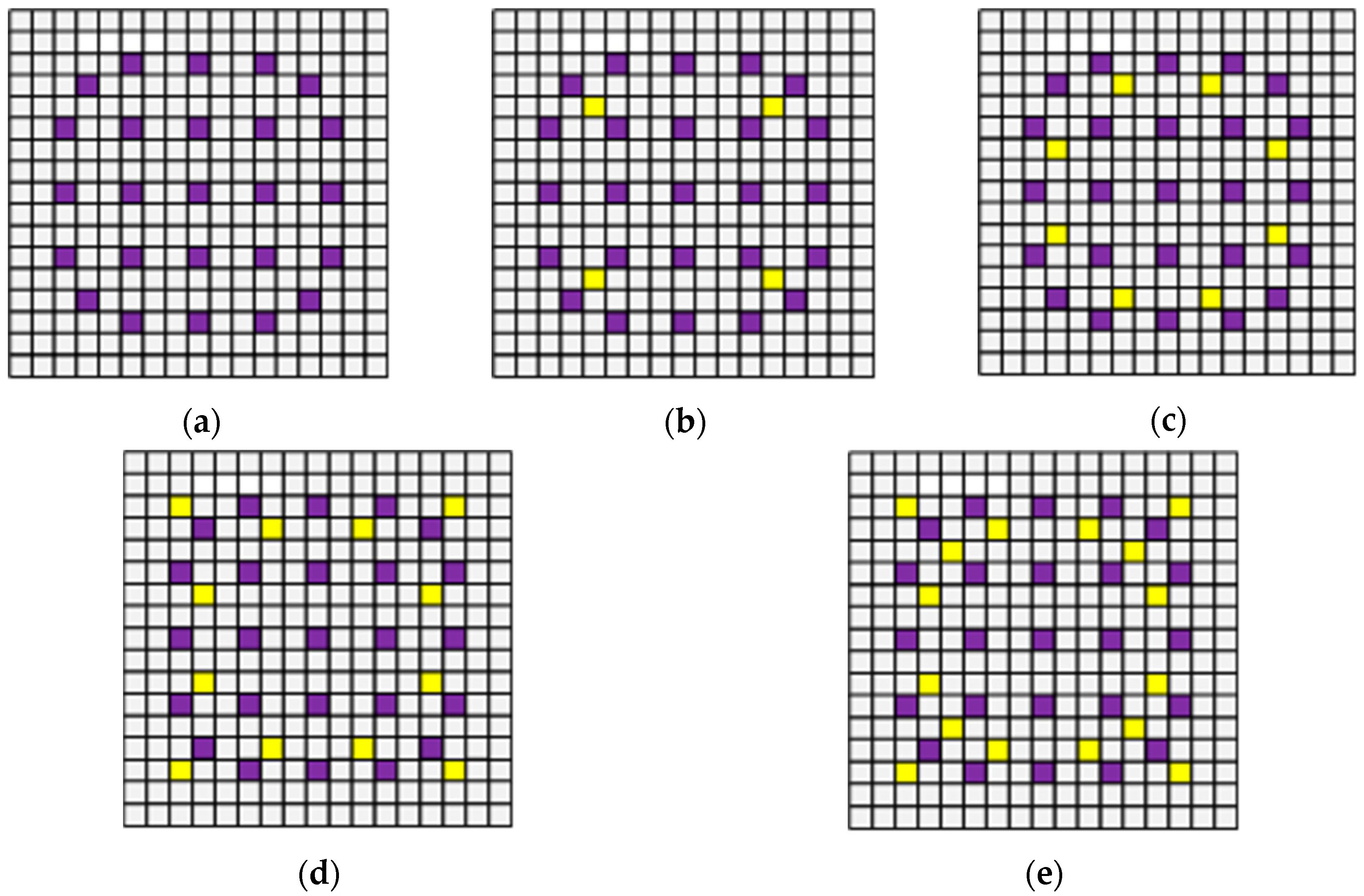
Considering that the enrichment of PWR fuel ranges between 1.8% and 4.95% and that the fuel is not axially zoned, the commonly used burnable poison in PWRs is Gd2O3, with a content ranging from 6% to 12%, uniformly dispersed within the UO2 fuel pellets. Due to the lower melting point of the Gd2O3+UO2 sintered material, the fuel enrichment in burnable poison rods is usually lower than that in pure fuel rods. Therefore, when the fuel rod enrichment is between 1.8% and 4.0%, the fuel enrichment in gadolinium rods is 0.711%; when the fuel enrichment exceeds 4.0%, to prevent a significant temperature difference between gadolinium rods and fuel rods that could lead to a higher power peaking factor in the assembly and reduced economic efficiency, the fuel enrichment in gadolinium rods is adjusted to 2.0%. The burnable poison arrangement is characterized by 0, 4, 8, 12, and 16 burnable poison rods, with the dimensions of the gadolinium rods matching those of the UO2 fuel rods. The specific model of the assembly is shown in Figure 2. The main design variables of the assembly are fuel enrichment, burnable poison content, and arrangement. The specific arrangements and corresponding feature spaces are listed in Table 1. Other design parameters, such as cladding material, uranium–water lattice geometry, assembly pitch, and the number of guide tubes, adopt the design parameters of the AFA-3G assembly [20]. The specific geometric parameters of the assembly are listed in Table 2 [21].
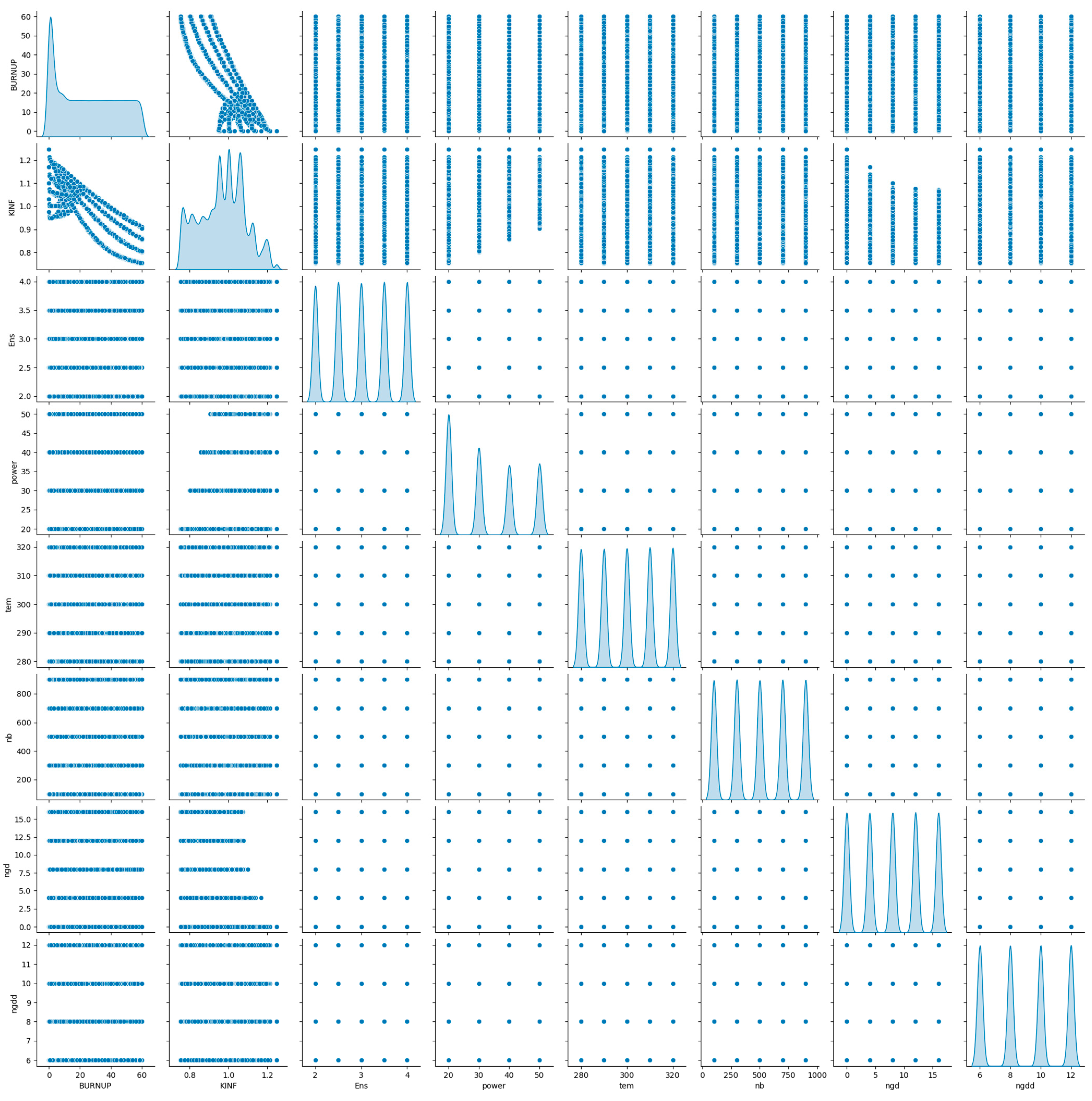
Based on the different high-dimensional initial conditions selected in Table 1, all assembly schemes are calculated using the DRAGON 4.1 code. The infinite multiplication factor kinf of the assemblies is chosen as the parameter to be predicted. The feature distributions of the high-dimensional data and the infinite multiplication factor kinf of the assemblies are plotted, with the feature distribution diagram shown in Figure 3.
By selecting different high-dimensional initial conditions, all assembly schemes are calculated using the DRAGON 4.1 program to obtain the dataset needed for neural network training. This dataset contains seven features (Burnup, Enrichment, Power, Temperature, Boron concentration, Burnable poison arrangement form, Burnable poison enrichment) and one target variable (kinf). Scatter plots or kernel density estimation (KDE) plots are created for these eight features. Through Figure 3, the relationships between each feature and the distribution differences among different categories can be intuitively observed.
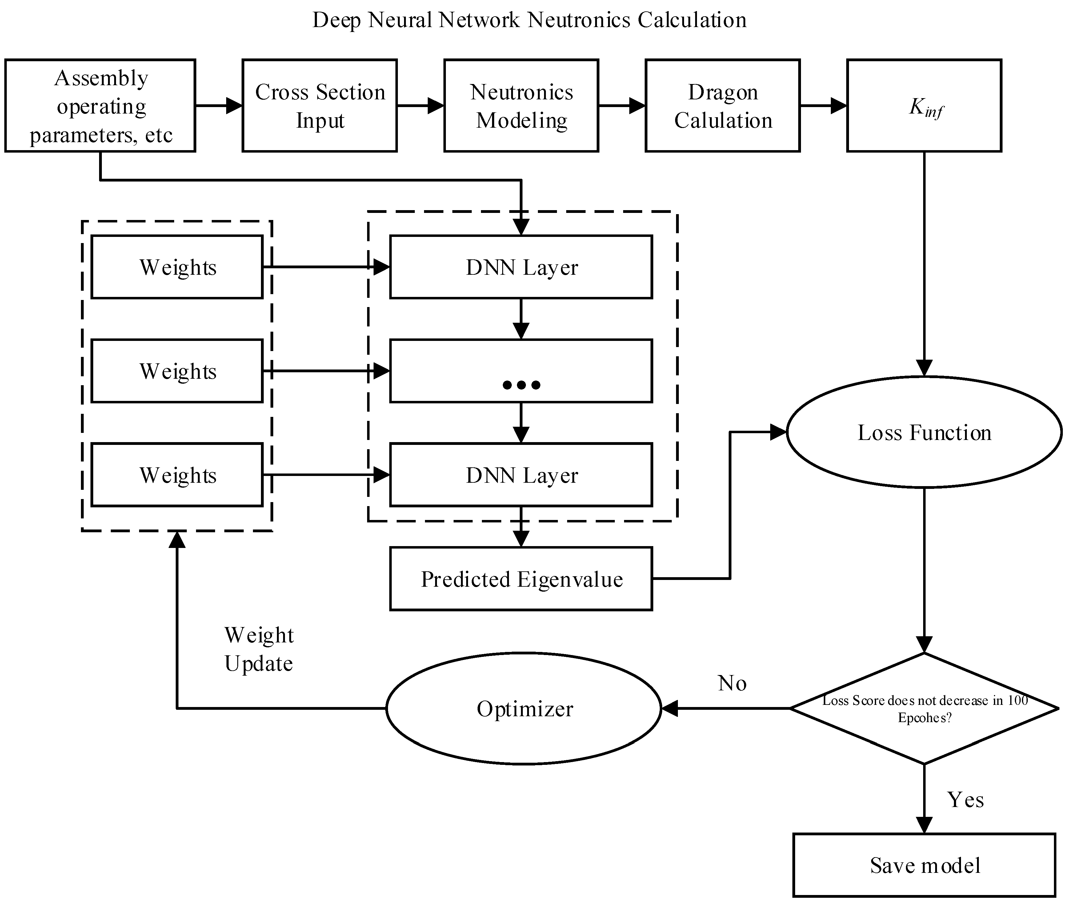
The entire framework process of this study is visualized as shown in Figure 4. First, high-fidelity calculations are performed on the sample set using the DRAGON 4.1 code. Next, the dataset is classified and divided into training, validation, and test sets. Subsequently, the training set is used to establish a high-dimensional neutron transport neural network model, and hyperparameters are continually adjusted to obtain the optimal weight parameters based on evaluation metrics. Finally, the test set is used to test the trained model and verify its generalization ability.
The software environment for the experiments in this study includes the following: Windows 10 operating system, Anaconda3 platform, Python 3.7, CUDA version 11.2, and TensorFlow 2.9.0 as the deep learning framework. The hardware environment comprises an Intel(R) Core(TM) i7-14700KF CPU with a clock speed of 3.40 GHz and a single NVIDIA GeForce RTX 3090 GPU with 24 GB of memory. The optimization algorithm used is Adam, with an initial learning rate set to 5.0 × 10⁻³, a batch size of 1024, and 5000 epochs. In the EarlyStopping function, the patience parameter is set to 100, meaning the model’s training will stop and save the model parameters if there is no improvement in the prediction performance over 100 epochs.
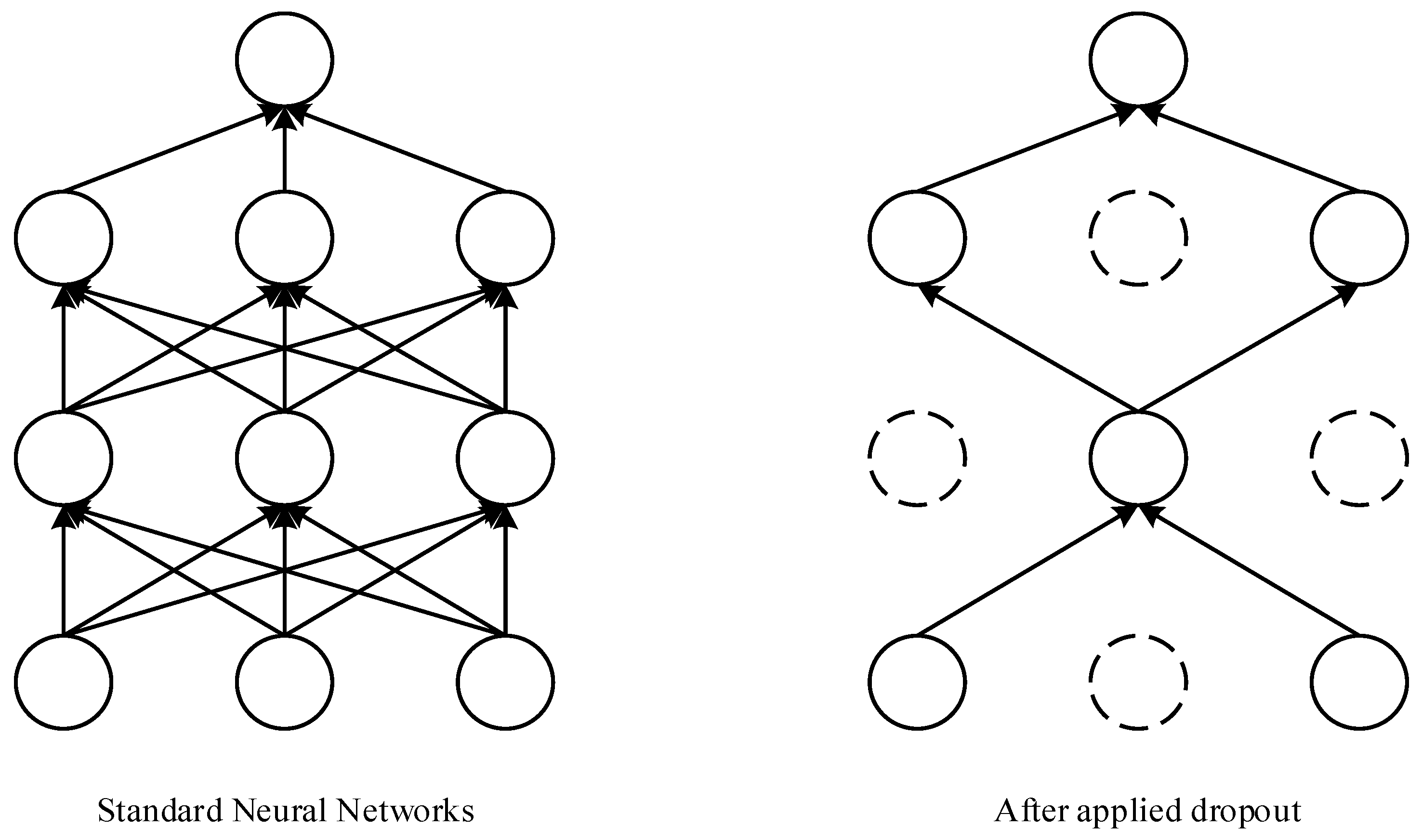
The trained model is validated using the validation set, and dropout layers are utilized to prevent overfitting. Based on Occam’s Razor principle [22], if there are two explanations for an occurrence, the simpler one is usually better, meaning the one with fewer assumptions. Given some training data and a network architecture, many sets of weight values (i.e., many models) can explain the data, and simpler models are less likely to overfit compared to complex models. Dropout [22] refers to randomly removing certain units from the neural network during training, which means that each mini-batch effectively trains a different network. The mechanism is shown in Figure 5, where random neuron dropout helps prevent the model from overfitting.
A random selection of 60% of the feature set is used as the training set, 20% as the validation set, and the remaining 20% as the test set. A high-dimensional neutron transport assembly infinite multiplication factor kinf model is established using the open-source TensorFlow framework, and regression training is conducted using the training set. By continuously adjusting the hyperparameters of the neural network to minimize the loss function, an experimental model that meets engineering requirements is finally obtained.

4. Results Analysis

In this study, the Mean Squared Error (MSE) function and the Mean Absolute Error (MAE) function are used as the loss functions to construct the prediction model for the high-dimensional neutron transport assembly infinite multiplication factor kinf. The calculation formulas are shown in Equations (2)–(5), where N is the set size, y i is the actual value, and y ^ i is the predicted value, A B S is the absolute error, R E L is the relative error [23,24]. From these formulas, it can be concluded that the closer the loss function is to 0, the better the prediction effect. By setting the model hyperparameters and conducting numerous experiments, an optimal set of hyperparameters for the model is obtained, as shown in Table 3.
M S E = 1 N 1 N y i y ^ i 2
M A E = 1 N 1 N y i y ^ i
A B S = y i y ^ i
R E L = y i y ^ i y ^ i 100 %
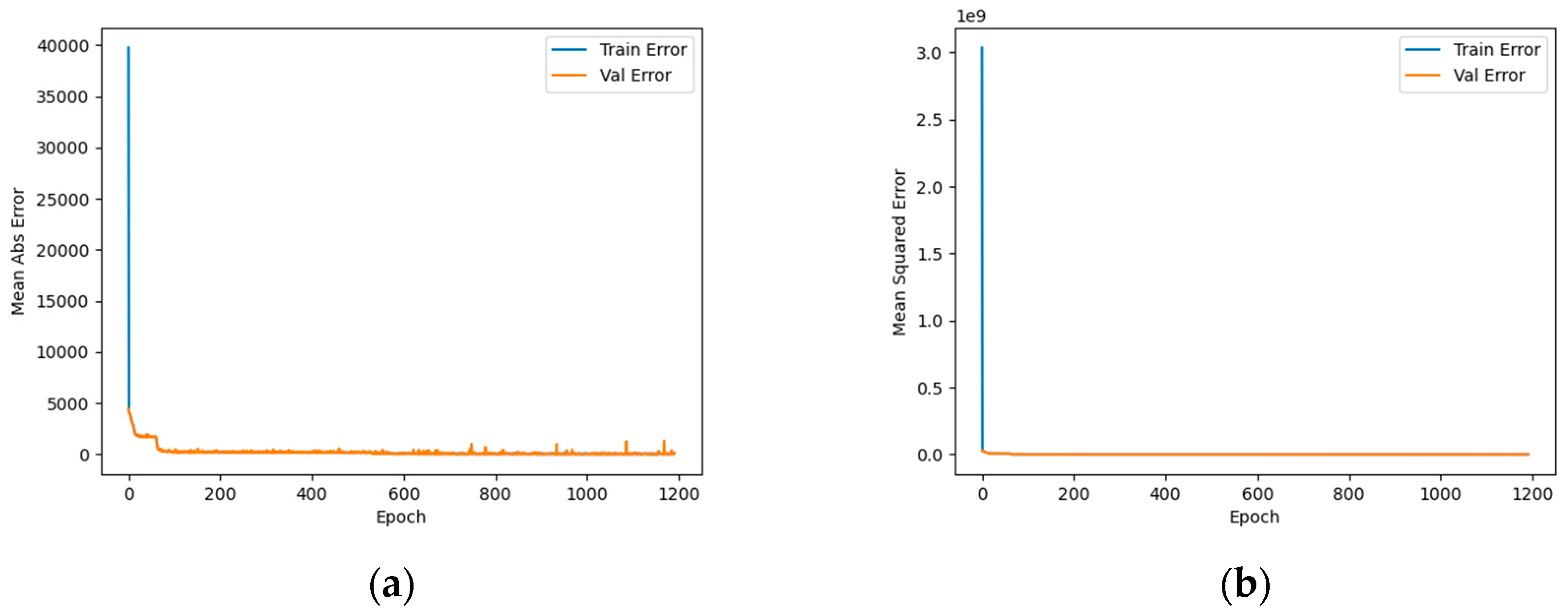
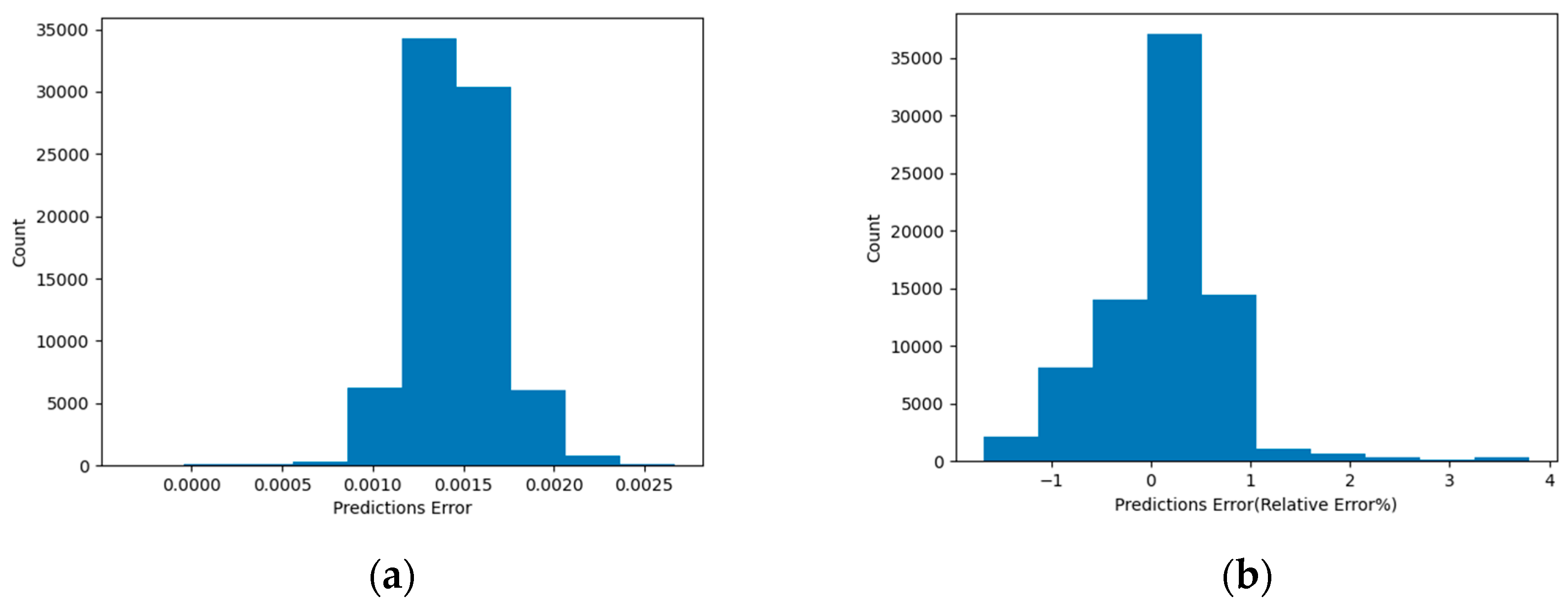
Based on the hyperparameters shown in Table 3, a high-dimensional neutron transport neural network model is established to monitor the training process. The results are shown in Figure 6 (orange curve represents the training process; blue curve represents the validation process). From the training process, it can be seen that the loss function tends to stabilize. The model is tested on the test set to verify its generalization ability, and the results are shown in Figure 7. The results indicate that for the high-dimensional neutron transport problem, the constructed model has an average test error of 145.71 pcm, a maximum error of 267.10 pcm, and a maximum relative error of less than 3.5%, all of which are within the engineering error standards of 500 pcm and 5%. This verifies the feasibility of establishing a prediction model for the infinite multiplication factor kinf of high-dimensional neutron transport assemblies using a deep neural network.
This study aims to establish a data-driven model for solving high-dimensional neutron transport equations. Using the AFA-3G assembly dataset obtained from DRAGON4.1 for deep learning neural network modeling, several key findings were obtained. Firstly, this study demonstrates that the high-dimensional neutron transport equation-solving model can significantly improve the efficiency of solving neutronic parameters in assemblies. Specifically, for the high-dimensional neutron transport problem of the AFA-3G assembly, the constructed model yielded an average test error of 145.71 pcm, a maximum error of 267.10 pcm, and a maximum relative error of less than 3.5%, all of which are below the engineering error standards of 500 pcm and 5%. These results can be attributed to the high accuracy of the neural network in parameter prediction, mainly due to its powerful nonlinear modeling capability. By using different activation functions, the neural network can capture and process complex nonlinear relationships within the data. Additionally, neural networks typically rely on large amounts of training data, from which they learn and generalize the patterns and rules within the data. In a multi-layer structure, each layer gradually extracts higher-level features from the data, enhancing the model’s expressive power. The backpropagation algorithm allows the neural network to adaptively adjust parameters and continuously optimize the model, thereby improving prediction accuracy. This combination of nonlinear modeling, feature extraction, and adaptive learning enables neural networks to excel in handling complex prediction tasks. Compared to the existing literature, this study further explores the feasibility of neural networks in solving high-dimensional neutron transport equations. Although this study reaches positive conclusions, some limitations remain. Firstly, the research currently focuses only on the AFA-3G assembly, and the results are not yet generalizable. Secondly, the data used in this study are derived solely from simulation software; although the physical parameters in the simulation software are not significantly different from real values, there are still some discrepancies in the specific values. Therefore, future research should consider model transfer and the use of real datasets to validate the conclusions of this study.

5. Conclusions

To explore the feasibility of artificial intelligence in nuclear engineering design and computation, this study calculates 60,000 samples with high-dimensional parameters using the DRAGON4.1 code, using the infinite multiplication factor kinf as the prediction parameter. Randomly, 36,000 samples are set aside as the test set, 12,000 samples as the validation set, and the remaining 12,000 samples as the training set. Subsequently, a deep neural network model is constructed, and parameters such as MAE and MSE are used to evaluate the model’s fitting performance. The trained model is then used to predict the infinite multiplication factor kinf for the test set samples, and the accuracy is assessed. Experimental results show that the average error between the predicted infinite multiplication factor kinf of the deep neural network model for high-dimensional data and the reference value is 145.71 pcm, the maximum error is 267.10 pcm, and the maximum relative error is less than 3.5%, all within the engineering error standards of 500 pcm and 5%. This preliminarily verifies the feasibility of solving high-dimensional neutron transport equations using a data-driven artificial intelligence approach, providing a new option for engineering design and practical engineering calculations.

Author Contributions

Conceptualization, J.L. and Z.P.; Methodology, J.L. and Z.P.; Software, Z.N.; Validation, J.H. and H.H.; Formal analysis, J.L. Investigation, Z.P. and J.H.; Resources, H.H. and J.X.; Data curation, J.L.; Writing—original draft, J.L. and Z.P.; Writing—review & editing, J.L. and Z.P.; Visualization, Z.N. and Z.P.; Supervision, J.X. and T.Y.; Project administration, J.X. and T.Y.; Funding acquisition, Z.P. and T.Y. All authors have read and agreed to the published version of the manuscript.

Funding

This research was funded by National Natural Science Foundation of China (no. U2267207), and Hunan Provincial Department of Education Key Teaching Reform Project (202401001561).

Data Availability Statement

The datasets generated during and/or analyzed during the current study are available from the corresponding author on reasonable request.

Conflicts of Interest

The authors declare that they have no conflicts of interest.

References

  1. Bethe, H.A. Nuclear physics B. Nuclear dynamics, theoretical. Rev. Mod. Phys. 1937, 9, 69. [Google Scholar] [CrossRef]
  2. Ren, C.; He, L.; Lei, J.; Liu, J.; Huang, G.; Gao, K.; Qu, H.; Zhang, Y.; Li, W.; Yang, X.; et al. Neutron transport calculation for the BEAVRS core based on the LSTM neural network. Sci. Rep. 2023, 13, 14670. [Google Scholar] [CrossRef]
  3. Lei, J.; Xie, J.; Chen, Z.; Yu, T.; Yang, C.; Zhang, B.; Zhao, C.; Li, X.; Wu, J.; Zhuang, H.; et al. Validation of Doppler Temperature Coefficients and Assembly Power Distribution for the Lattice Code KYLIN V2.0. Front. Energy Res. 2021, 9, 801481. [Google Scholar] [CrossRef]
  4. Capilla, M.; Talavera, C.; Ginestar, D.; Verdú, G. Validation of the SHNC time-dependent transport code based on the spherical harmonics method for complex nuclear fuel assemblies. J. Comput. Appl. Math. 2020, 375, 112814. [Google Scholar] [CrossRef]
  5. Zhang, G.; Li, Z. Marvin: A parallel three-dimensional transport code based on the discrete ordinates method for reactor shielding calculations. Prog. Nucl. Energy 2021, 137, 103786. [Google Scholar] [CrossRef]
  6. Rahman, A.; Lee, D. Incorporation of anisotropic scattering into the method of characteristics. Nucl. Eng. Technol. 2022, 54, 3478–3487. [Google Scholar] [CrossRef]
  7. Dunn, W.L.; Shultis, J.K. Exploring Monte Carlo Methods; Elsevier: Amsterdam, The Netherlands, 2022. [Google Scholar] [CrossRef]
  8. Chu, T.-N.; Phan, G.T.; Tran, L.Q.L.; Bui, T.H.; Do, Q.B.; Dau, D.-T.; Nguyen, K.-C.; Nguyen, N.-D.; Nguyen, H.-T.; Hoang, V.-K.; et al. Sensitivity and uncertainty analysis of the first core of the DNRR using MCNP6 and new nuclear data libraries. Nucl. Eng. Des. 2024, 419, 112986. [Google Scholar] [CrossRef]
  9. Sandhu, H.K.; Bodda, S.S.; Gupta, A. A future with machine learning: Review of condition assessment of structures and mechanical systems in nuclear facilities. Energies 2023, 16, 2628. [Google Scholar] [CrossRef]
  10. Lei, J.; Zhou, J.; Zhao, Y.; Chen, Z.; Zhao, P.; Xie, C.; Ni, Z.; Yu, T.; Xie, J. Prediction of burn-up nucleus density based on machine learning. Int. J. Energy Res. 2021, 45, 14052–14061. [Google Scholar] [CrossRef]
  11. Qi, B.; Liang, J.; Tong, J. Fault diagnosis techniques for nuclear power plants: A review from the artificial intelligence perspective. Energies 2023, 16, 1850. [Google Scholar] [CrossRef]
  12. Lei, J.; Yang, C.; Ren, C.; Li, W.; Liu, C.; Sun, A.; Li, Y.; Chen, Z.; Yu, T. Development and validation of a deep learning-based model for predicting burnup nuclide density. Int. J. Energy Res. 2022, 46, 21257–21265. [Google Scholar] [CrossRef]
  13. Pikus, M.; Wąs, J. Using Deep Neural Network Methods for Forecasting Energy Productivity Based on Comparison of Simulation and DNN Results for Central Poland—Swietokrzyskie Voivodeship. Energies 2023, 16, 6632. [Google Scholar] [CrossRef]
  14. Xie, Y.; Wang, Y.; Ma, Y. Boundary dependent physics-informed neural network for solving neutron transport equation. Ann. Nucl. Energy 2024, 195, 110181. [Google Scholar] [CrossRef]
  15. Wang, Y.; Chi, H.; Ma, Y. Nodal expansion method based reduced-order model for control rod movement. Ann. Nucl. Energy 2024, 198, 110279. [Google Scholar] [CrossRef]
  16. Liu, B.; Lei, J.; Xie, J.; Zhou, J. Development and Validation of a Nuclear Power Plant Fault Diagnosis System Based on Deep Learning. Energies 2022, 15, 8629. [Google Scholar] [CrossRef]
  17. Tran, V.D.; Lam, D.K.; Tran, T.H. Hardware-based architecture for DNN wireless communication models. Sensors 2023, 23, 1302. [Google Scholar] [CrossRef]
  18. Wu, L.; Zhang, Z.; Yang, X.; Xu, L.; Chen, S.; Zhang, Y.; Zhang, J. Centroid Optimization of DNN Classification in DOA Estimation for UAV. Sensors 2023, 23, 2513. [Google Scholar] [CrossRef]
  19. Marleau, G.; Hébert, A.; Roy, R. A User Guide for DRAGON Version 4; Institute of Genius Nuclear, Department of Genius Mechanical, School Polytechnic of Montreal: Montreal, QC, Canada, 2011. [Google Scholar]
  20. Xiaohui, W. Analysis and Research on Diagnosis Methods of AFA 3G Fuel Assembly Leakage. In Proceedings of the 2017 25th International Conference on Nuclear Engineering, Shanghai, China, 2–6 July 2017; American Society of Mechanical Engineers: New York, NY, USA, 2017; Volume 57793, p. V001T01A001. [Google Scholar]
  21. Li, J.; Qiao, S.; Ren, J.; Yu, X.; Tian, R.; Tan, S. Detailed comparison of the characteristics of mixing and subchannel vortex induced by different spacer grids. Prog. Nucl. Energy 2023, 166, 104962. [Google Scholar] [CrossRef]
  22. Lei, J.; Ren, C.; Li, W.; Fu, L.; Li, Z.; Ni, Z.; Li, Y.; Liu, C.; Zhang, H.; Chen, Z.; et al. Prediction of crucial nuclear power plant parameters using long short-term memory neural networks. Int. J. Energy Res. 2022, 46, 21467–21479. [Google Scholar] [CrossRef]
  23. Lei, J.; Chen, Z.; Zhou, J.; Yang, C.; Ren, C.; Li, W.; Xie, C.; Ni, Z.; Huang, G.; Li, L.; et al. Research on the preliminary prediction of nuclear core design based on machine learning. Nucl. Technol. 2022, 208, 1223–1232. [Google Scholar] [CrossRef]
  24. Ren, C.; Li, H.; Lei, J.; Liu, J.; Li, W.; Gao, K.; Huang, G.; Yang, X.; Yu, T. CNN-lstm-based model to fault diagnosis for CPR1000. Nucl. Technol. 2023, 209, 1365–1372. [Google Scholar] [CrossRef]
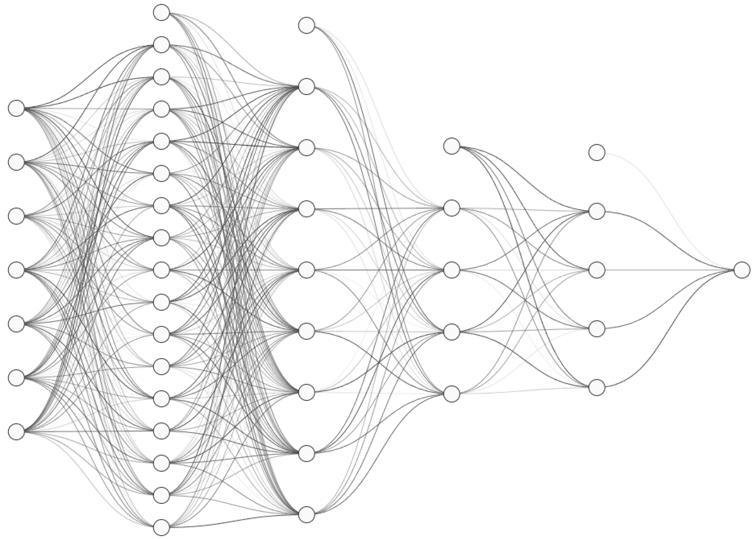
Figure 1. Fuel assembly geometric distribution.
Energies 17 04153 g001
Figure 2. The arrangement plan of burnable poison: (a) 0 burnable poison rods; (b) 4 burnable poison rods; (c) 8 burnable poison rods; (d) 12 burnable poison rods; (e) 16 burnable poison rods.
Energies 17 04153 g002
Figure 3. Feature distribution diagram.
Energies 17 04153 g003
Figure 4. The general framework of the deep learning model applied to solving high-dimensional neutron transport equations.
Energies 17 04153 g004
Figure 5. Dropout mechanism diagram.
Energies 17 04153 g005
Figure 6. Model training loss function value diagram: (a) MAE; (b) MSE.
Energies 17 04153 g006
Figure 7. Model prediction error distribution diagram: (a) Prediction absolute error; (b) Prediction relative error.
Energies 17 04153 g007
Table 1. Specific parameters of assembly independent variables.
Assembly Independent VariablesValueFeature Name
Burnup (Gw·d/tU)0–60/Step 0.5BURNUP
Enrichment (%)2–4/Step 0.5ENS
Power (W/cm)20–50/Step 10power
Temperature (°C)280–320/Step 10tem
Boron concentration (ppm)100–900/Step 200nb
Burnable poison arrangement form (rod)0–16/Step 4ngd
Burnable poison enrichment (%)6–12/Step 2ngdd
Table 2. Fuel assembly geometry parameters.
Assembly Geometry ParameterValue
Outer surface diameter of cladding/cm0.95
Cladding materialM5
UO2 pellet diameter/cm0.8192
Gap gasHelium
Core active section height/cm365.8
Burnable poison arrangement form (rod)0–16/Step 4
Fuel rod center distance/cm1.26
Number of assembly grids17 × 17
Fuel assembly center distance/cm21.504
Number of tubes per assembly25
Number of UO2 fuel pins per assembly264
UO2 pellet density/g/cm310.412
Water density/g/cm30.9983
M5 density/g/cm36.5
Table 3. Optimum DNN hyperparameters.
ItemValueItemValue
Hidden Layers6Input ScalingMax-Min
Nodes per layer512, 256, 128, 64, 4, 1ActivationReLU
Dropout (after 1st layer)0.3OptimizerAdam
Loss FunctionMSEEpochs5000
Batch Size1024Training/Validation/Testing Samples6:2:2
Disclaimer/Publisher’s Note: The statements, opinions and data contained in all publications are solely those of the individual author(s) and contributor(s) and not of MDPI and/or the editor(s). MDPI and/or the editor(s) disclaim responsibility for any injury to people or property resulting from any ideas, methods, instructions or products referred to in the content.