Review

Advanced Deep Learning Techniques for Battery Thermal Management in New Energy Vehicles

1
National Key Laboratory of Automotive Chassis Integration and Biomimetics, Jilin University, Changchun 130025, China
2
College of Automotive Engineering, Jilin University, Changchun 130025, China
*
Author to whom correspondence should be addressed.
Energies 2024, 17(16), 4132; https://doi.org/10.3390/en17164132
Submission received: 25 July 2024 / Revised: 12 August 2024 / Accepted: 16 August 2024 / Published: 19 August 2024
(This article belongs to the Special Issue New Energy Vehicles: Battery Management and System Control)

Abstract

:
In the current era of energy conservation and emission reduction, the development of electric and other new energy vehicles is booming. With their various attributes, lithium batteries have become the ideal power source for new energy vehicles. However, lithium-ion batteries are highly sensitive to temperature changes. Excessive temperatures, either high or low, can lead to abnormal operation of the batteries, posing a threat to the safety of the entire vehicle. Therefore, developing a reliable and efficient Battery Thermal Management System (BTMS) that can monitor battery status and prevent thermal runaway is becoming increasingly important. In recent years, deep learning has gradually become widely applied in various fields as an efficient method, and it has also been applied to some extent in the development of BTMS. In this work, we discuss the basic principles of deep learning and related optimization principles and elaborate on the algorithmic principles, frameworks, and applications of various advanced deep learning methods in BTMS. We also discuss several emerging deep learning algorithms proposed in recent years, their principles, and their feasibility in BTMS applications. Finally, we discuss the obstacles faced by various deep learning algorithms in the development of BTMS and potential directions for development, proposing some ideas for progress. This paper aims to analyze the advanced deep learning technologies commonly used in BTMS and some emerging deep learning technologies and provide new insights into the current combination of deep learning technology in new energy trams to assist the development of BTMS.

1. Introduction

The substantial increase in the number of traditionally fueled vehicles has led to a sharp rise in the proportion of carbon dioxide emissions from the transportation sector, exacerbating global warming [1,2]. With the growing awareness of environmental protection and the increasing international concern for environmental issues, controlling carbon dioxide emissions has become a critical agenda. Against this backdrop, the development of electric and other new energy vehicles is flourishing [3], and some countries have included the development of new energy vehicles in their national strategies [4,5]. New energy vehicle technology consists of technologies such as hybrid electric vehicles (HEV), battery electric vehicles (BEV), and fuel cell electric vehicles (FCEV), which are considered alternative technologies to traditional internal combustion engine vehicles (ICEV) [6].
Lithium batteries, with their high efficiency, high energy density, long lifespan, low self-discharge rate, and minimal memory effect, have become the ideal power source for new energy vehicle powertrains [7,8,9,10]. As illustrated in Figure 1, the working principle involves electrons moving from the anode to the cathode during discharge, with lithium atoms deposited between carbon layers at the anode losing electrons and diffusing towards the cathode’s electrolyte. During the charging process, this process occurs in the opposite direction [10,11,12]. However, lithium-ion batteries are highly sensitive to temperature changes throughout their service life [13,14]. Heat is generated within lithium batteries due to the chemical reactions during charging and discharging. If not properly managed, uneven heat distribution can lead to localized high temperatures, which can result in reduced battery performance, shortened lifespan, and even safety hazards [9,13,15]. Additionally, low temperatures in extreme environments can severely decrease the battery’s power and energy output [8]. Therefore, a Battery Thermal Management System (BTMS) is crucial for maintaining the temperature of batteries in new energy vehicles. It maximizes the performance of the lithium battery by maintaining the ideal temperature range of the battery and improving its temperature stability, and it effectively prevents the internal temperature rise caused by operation and the low temperatures caused by external environments, thus preventing damage to the batteries from these adverse factors [8,9,14,16,17,18].
In the research and design of an efficient BTMS, numerical simulation methods such as Computational Fluid Dynamics (CFDs) are commonly employed to obtain parameters like internal temperature fields and medium flow fields, which are then used to evaluate and improve the design, optimizing flow channel structures [20,21]. However, numerical simulation methods require substantial time and computational costs [21,22], hindering the efficient progress of BTMS design. Although the equivalent circuit model and lumped model are efficient and simplified models, they cannot provide detailed temperature distribution and heat flow path inside the battery, so they may not be accurate enough to design an accurate thermal management system. At the same time, these models often make it difficult to judge the future trend of battery parameters according to historical data [23,24]. Additionally, in the actual operation of new energy vehicles, the thermal runaway safety issues of batteries remain a key focus for BTMS [25]. Quickly and accurately estimating the battery’s thermal properties, such as temperature and heat generation rate, along with its electrical properties, including current, voltage, and state of charge, is essential for assessing its operational state. This capability is crucial for the BTMS to provide timely early warnings and control adjustments. Addressing this challenge is a major focus in ensuring the thermal safety of batteries in new energy vehicles. With the rapid development of artificial intelligence (AI) technology in recent years, deep learning (DL), as one of the hottest research trends in the field of AI, has developed swiftly [26], and its application in the field of thermal management for new energy vehicle batteries is increasing. Deep learning models, which are multi-layer Artificial Neural Network (ANN) models, have demonstrated efficient predictive performance in dealing with nonlinear problems such as battery heat generation and transient temperature fields [27,28,29]. After full learning, deep learning models can often output calculation results instantaneously while ensuring considerable accuracy. They often have obvious advantages over CFDs in calculation speed and computing power requirements. Using deep learning techniques to optimize BTMS design can save considerable computing resources [30]. The rapid predictive nature of deep learning models makes them a key technology for real-time monitoring and state judgment of battery parameters. Furthermore, with the introduction of advanced deep learning optimization algorithms such as Convolutional Neural Network (CNN) [31], Long Short-Term Memory network (LSTM) [32], Gated Recurrent Unit (GRU) [33], and Generative Adversarial Network (GAN) [34], deep learning’s role in assisting BTMS design research and applications is continuously deepening. These algorithms show excellent performance in handling spatial temperature distribution and long-time series of current and voltage features and make it possible for BTMS to predict the future state of the battery according to the spatial history information. The introduction of these algorithms provides strong support for the design of BTMS. Through deep learning technology, the working state of batteries during the operation of new energy vehicles can be more accurately predicted and judged, accelerating the design optimization of BTMS and thereby enhancing the safety of new energy vehicles and the performance of BTMS.
The contributions of this review and the structure of the article are as follows: Section 2 provides a detailed introduction to the basic algorithms in deep learning and the principles of related optimization algorithms. Section 3 reviews the principles of various advanced deep learning algorithms and their applications in recent years to address issues in battery thermal management and thermal safety, as well as in assisting the design of thermal management systems. This includes applications in estimating aspects such as temperature, heat generation, system performance, State of Charge (SOC), and voltage and elucidates the characteristics of these deep learning methods. Section 4 briefly introduces a recently proposed novel deep learning algorithm (KAN) [35], as well as some advanced deep learning algorithms not mentioned in previous reviews [8,16,22], such as Diffusion Model and Transformer [36,37]. It analyzes the advantages of these methods and their potential applications in battery thermal management. Section 5 summarizes some of the current deep learning techniques used in BTMS. Section 6 discusses the current obstacles in the application of deep learning algorithms in battery thermal management and provides some feasible solutions and development directions for future research.

2. A Basic Introduction to Deep Learning

2.1. Concepts of Deep Learning

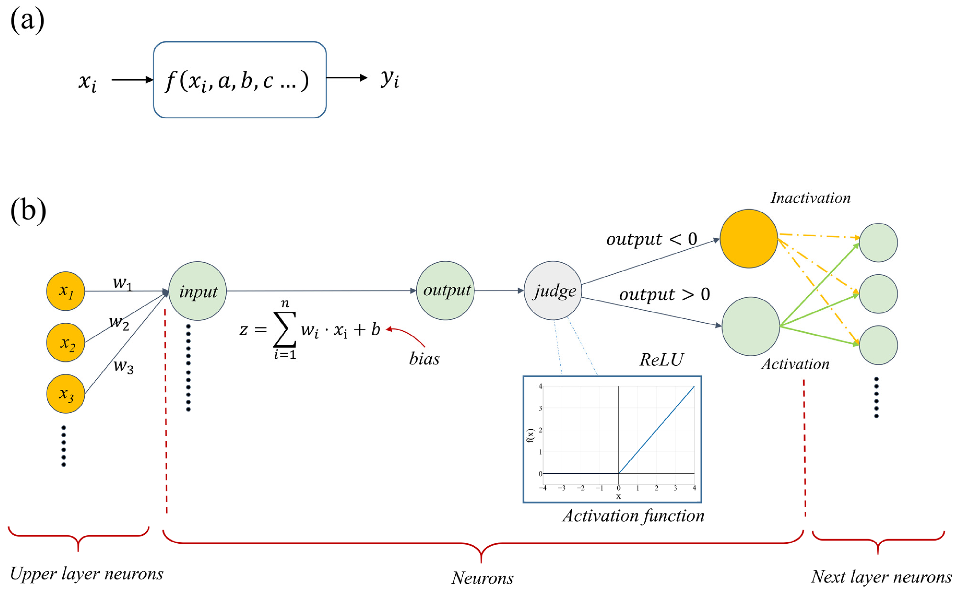
Deep learning’s complexity, often likened to a ‘black box’, arises from its extensive parameter set [38]. Figure 2a illustrates this as an intricate function, f ( x i , a , b , c ) , where x i denotes the input variables and a , b , c symbolizes the model’s parameters. The model processes these inputs x i to produce outputs y i . The ‘deep’ in deep learning signifies the presence of multiple layers within the network’s architecture, with each neuron functioning as a feature-processing unit. Figure 2b shows that each neuron receives input features, applies weights to them, and sums the results [39]. A bias is commonly added to this sum, and the ReLU activation function determines the neuron’s activation state: if the sum is less than zero, the neuron remains inactive; if greater, it activates and propagates the features to the next layer.

2.2. Loss Function

To describe the discrepancy between the output of a deep learning model and the target values, we employ loss functions to evaluate the performance of the generated model [40]. In the context of regression problems in deep learning, several commonly used loss functions include Mean Absolute Error (MAE), Mean Square Error (MSE), Root Mean Square Error (RMSE), Huber Loss, and LogCosh Loss. Their formulas are shown in Equations (1)–(5), as follows:
M A E = 1 n i = 1 n | y i y i |
M S E = 1 n i = 1 n ( y i y i ) 2
R M S E = 1 n · i = 1 n ( y i y i ) 2
H u b e r = { 1 2 n i = 1 n ( y i y i ) 2 , | y i y i | δ 1 2 n i = 1 n ( 2 δ | y i y i | δ 2 ) , | y i y i | > δ
L o g C o s h = 1 n i = 1 n log ( cosh ( y i y i ) ) , cosh ( x ) = e x + e x 2
where i is the index of the variable, y i is the predicted value, yi is the actual value, n is the total number of variables, δ is the parameter of the function, and x is the independent variable of the function.

2.3. Gradient Descent

Gradient descent is a fundamental optimization method used in training deep learning models. The core concept involves computing the gradient of the loss function with respect to a parameter in the deep learning model. This gradient information is then used to update the model’s parameters, steering them in the direction where the loss function decreases, thereby minimizing the model’s overall loss. This process can be described in Equations (6)–(8) [41], as follows:
g a = a L ( x i , y i , a , b , c )
δ a = l r · g a
a = a δ a
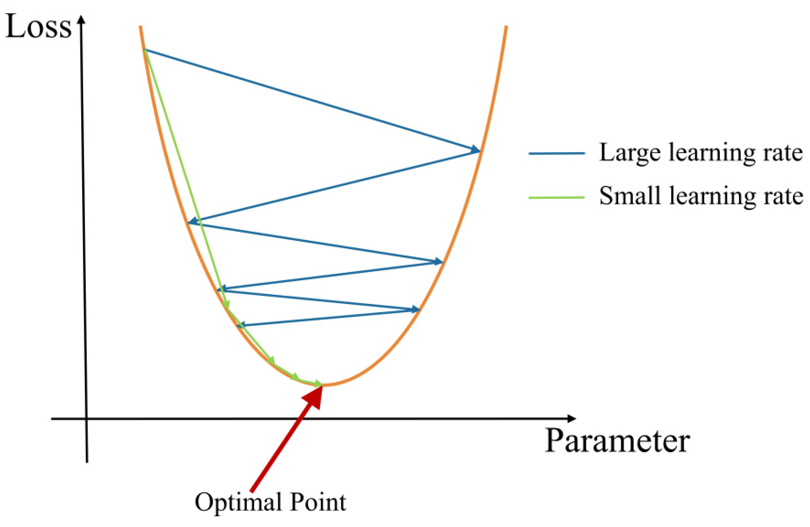
In gradient descent optimization, the loss function L ( x i , y i , a , b , c ) is minimized by updating the model parameter a based on the gradient g a of the loss with respect to the parameter. The update amount δ a is determined by the learning rate l r , which scales the gradient to adjust the step size. The updated parameters are denoted by a . As the model parameters evolve, the loss and its gradient decrease. As per Equation (7), a higher learning rate leads to larger parameter updates, potentially accelerating convergence but risking overshooting the optimal solution, as depicted in Figure 3. This can result in oscillations around the optimum, hindering stable convergence. On the other hand, a lower learning rate ensures more gradual updates, reducing the risk of oscillations but at the cost of slower convergence.

2.4. Stochastic Gradient Descent (SGD)

In deep learning, models often process multiple batches of data concurrently. Performing full dataset computations to determine the gradient mean for a single parameter update can be computationally intensive and may slow down the learning process [41]. To mitigate this, Stochastic Gradient Descent (SGD) [42] selects a random subset of the data for each update, calculating the gradient mean over this subset to update the model parameters. This method conserves computational resources and speeds up the training process [16].

2.5. Backpropagation

Furthermore, deep learning models leverage the backpropagation algorithm to uncover intricate patterns within extensive datasets, fine-tuning their internal parameters accordingly [43]. Backpropagation is an efficient technique for gradient computation. It initiates at the output layer, employs the chain rule to determine the error gradients for each layer, and stores these gradients. Utilizing these stored values, the algorithm calculates the error gradients for the parameters of the preceding layers. Finally, it updates the parameters of each layer through gradient descent, facilitating the model’s learning and adaptation [44].

2.6. Improved Optimization Method

In deep learning, SGD can guide the model in optimizing the direction of minimizing loss, but it has some drawbacks. For instance, as the model trains, the learning rate often needs to be manually adjusted to accommodate the varying demands for model parameter updates under different loss gradients, preventing the model from overfitting. Additionally, in deep learning, SGD tends to become stuck in local minima, making it difficult for the model to optimize.

2.6.1. Gradient Descent with Momentum

In deep learning, SGD is prone to become stuck at saddle points, where the gradient is zero but not at a global optimum of the parameters, causing the network parameters to oscillate near local optima and making it difficult to update towards the global optimum [41]. To adjust the learning speed and accelerate the convergence of deep learning, momentum-based stochastic gradient algorithms have been proposed [45,46]. As shown in Figure 4a, these methods retain the influence of the previous update direction on the next iteration. When facing a local optimum, the introduction of momentum can prevent parameter updates from being too small due to a shallow gradient, thus avoiding becoming stuck at local optima. At the same time, when dealing with high-curvature issues, as shown in Figure 4b, the update direction from the last parameters will restrict the current update direction, reducing the update amount and alleviating parameter oscillation. Momentum methods can speed up convergence and help parameters escape local optima when dealing with high-curvature and noisy gradients [46,47]. These principles can be referred to in Equations (6), (9) and (10) [41]:
m = γ · m + l r · g a
a = a m
where g a represents the partial derivative of the loss function with respect to the model parameter; a , m is the momentum term in the momentum gradient descent, which helps in accelerating the learning process; m is the updated momentum term after considering the influence of the previous update; l r is the learning rate, a hyperparameter that scales the update step; a denotes the updated model parameters after the application of the momentum method; and γ is a hyperparameter related to the momentum term, indicating the influence weight of the previous update direction on the current update direction.

2.6.2. Adaptive Gradient Algorithm (AdaGrad)

As parameters are continuously updated, they gradually converge on the optimal values. However, if the learning rate is kept constant, the magnitude of parameter updates may remain large even in the later stages of training, which can lead to overshoot and make it difficult for the model to converge [48]. The AdaGrad algorithm [49] addresses this issue by making the learning rate adaptive rather than fixed. As the model optimizes, the accumulated loss gradients cause the learning rate to decay progressively. These principles can be referenced in Equations (6) and (11)–(13) [50]:
S t = S t 1 + g a 2
l r = l r 0 · 1 S t + ε
a t = a t 1 l r · g a
where g a represents the partial derivative of the loss function with respect to the model parameter a. S t 1 is the sum of squared gradients accumulated after t 1 iterations of the model, and S t is the sum of squared gradients accumulated by the t-th iteration. lr is the current learning rate, l r 0 is the initial learning rate, and ε is a small constant added to prevent division by zero in Equation (12). According to the principle of the AdaGrad algorithm, the learning rate is determined by the accumulated squared loss gradients. As the model iterates, the sum of squared loss gradients continues to increase, causing the learning rate to decay over time. This aligns with the need for a lower learning rate in the later stages of deep learning iterations as the parameters approach the optimal point. Moreover, in AdaGrad, the adjustment of the learning rate is related to the accumulated squared gradients of the loss function corresponding to each parameter. As a result, different parameters may experience different rates of learning rate decay during training, allowing each parameter to adjust its learning rate independently according to its optimization needs. However, AdaGrad also has an undeniable issue: If the learning rate decays too rapidly during the iteration process, it may lead to a reduction in parameter updates in the later stages of model training, making it difficult for the model to converge.

2.6.3. Root Mean Square Propagation (RMSProp)

To a certain extent, the introduction of RMSProp has addressed the issue of premature learning rate decay in AdaGrad. Unlike AdaGrad, which accumulates the square of gradients over all past iterations, RMSProp focuses more on the gradient information from the recent iterations. It calculates the moving average of squared gradients using exponential decay, thus avoiding the monotonic decrease in learning rate that occurs with AdaGrad. These formulas can be referenced in Equations (6) and (12)–(14) [41,51]:
S t = β · S t 1 + ( 1 - β ) · g a 2
where β is the decay factor, which ranges from 0 to 1, and g a represents the partial derivative of the loss function with respect to the model parameter a. S t 1 is the exponentially weighted average of squared gradients at the iteration t 1 , while S t is the exponentially weighted average of squared gradients at the t-th iteration. RMSProp effectively mitigates the issue of premature learning rate decay caused by a single high loss gradient, as well as the problem of excessively low learning rates in later iterations due to monotonic decay, which can lead to insufficient optimization momentum. This adaptive learning rate adjustment method helps to maintain the algorithm’s dynamism and robustness during the training process.

2.6.4. Adaptive Moment Estimation (Adam)

Kingma et al. [52] proposed the Adaptive Moment Estimation (Adam) algorithm, which combines the advantages of RMSProp and AdaGrad. By updating the first and second moment estimates of the gradients, it achieves an adaptive learning rate that can effectively address the optimization issues associated with sparse gradients and non-stationary target functions [50]. The principles of this method can be referenced in Equations (6) and (15)–(19) [16,51]:
m t = β 1 · m t 1 + ( 1 β 1 ) · g a
S t = β 2 · S t 1 + ( 1 β 2 ) · g a 2
where β 1 , β 2 is the decay factor, which defaults to 0.9 and 0.999, g a is the partial derivative of the loss function with respect to the model parameters, and t is the number of current iterations. S t 1 , m t 1 is the exponential decay average of the squared gradient and the exponential decay average of the gradient at the number of t 1 iteration of the model.
m t = m t 1 β 1 t
S t = S t 1 β 2 t
a t = a t 1 l r S t + ε · m t
where m t , S t are the modified m t , S t . lr is the learning rate. ε is a small quantity in order to avoid the denominator being 0 in Equation (19).

2.7. Mixed-Precision Training

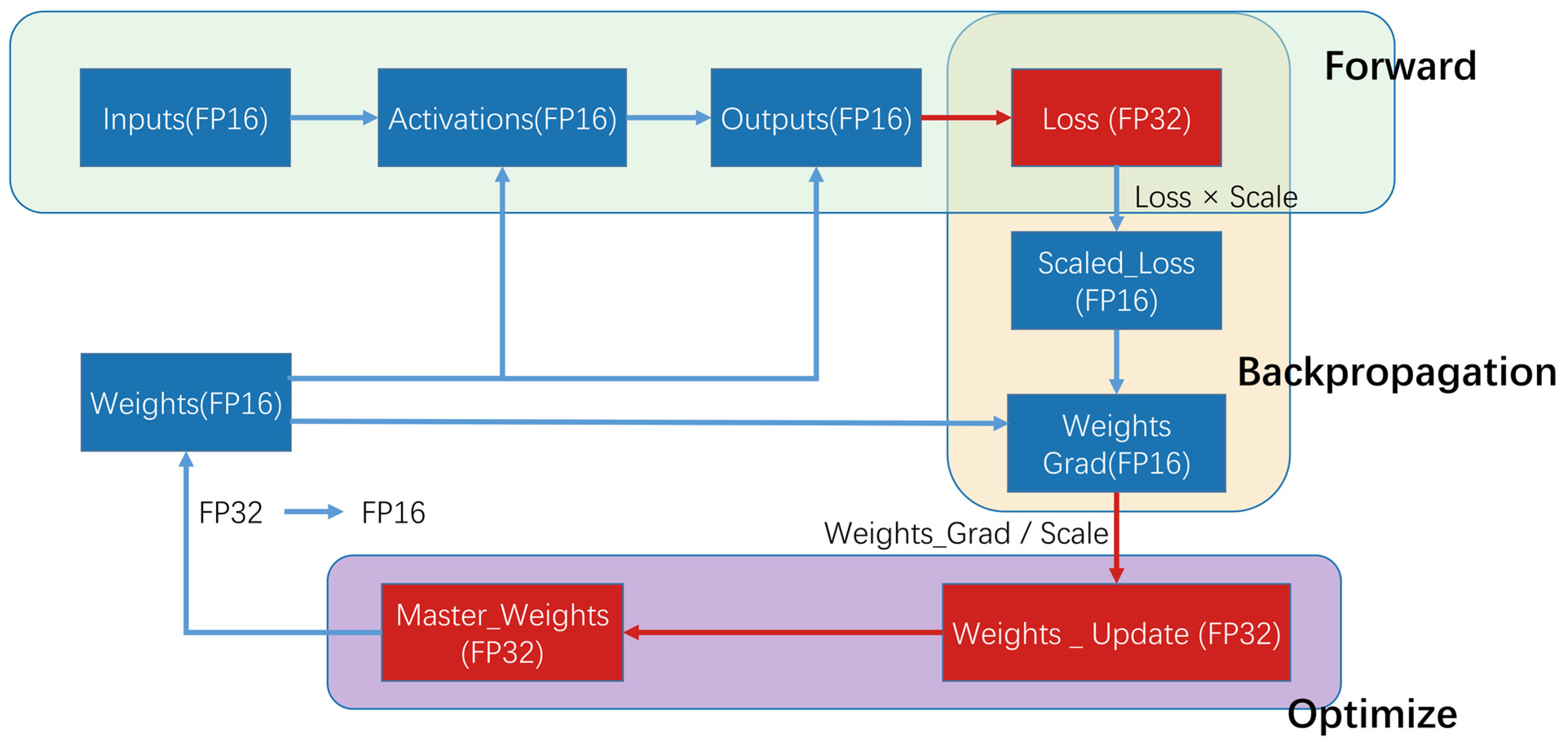
In most cases, deep learning models are trained using single-precision floating-point (FP32) arithmetic. During gradient computation, the large number of parameters in deep learning models increases computational workload and memory pressure due to the use of FP32. In 2017, mixed-precision training [53] was proposed, effectively alleviating the computational pressure and storage volume issues associated with FP32 operations. When training deep learning models with mixed precision, the combination of single-precision and half-precision floating-point (FP16) numbers leverages their respective advantages to accelerate training speed and reduce memory usage while ensuring accuracy [54]. The key techniques of mixed-precision training are threefold, as follows: weight backup, loss scaling, and precision accumulation.
As illustrated in Figure 5, during mixed-precision training, the model’s parameters are stored in FP16 format, while a copy of the weight parameters is kept in FP32 (referred to as Master_Weights) for updates during training. To prevent issues such as underflow caused by the use of FP16 in parameter updates, where gradients may become too small, and to reduce the impact of rounding errors on model performance, an appropriate scaling of the loss function can address these concerns. Specifically, the loss in FP32 format is multiplied by a scale factor to shift potentially overflowing fractional data, thus avoiding overflow issues when converting the loss to FP16 format. In mixed-precision training, matrix multiplication operations are performed using FP16, and the results are accumulated using FP32 data format before being converted back to FP16 for storage in memory. Currently, many deep learning frameworks [55,56] have integrated mixed-precision training. Utilizing mixed-precision training when training models on GPUs can effectively reduce GPU memory occupation and computational load, saving training time. With the same hardware, mixed-precision training can accommodate larger batch sizes, thereby accelerating model training and enhancing training performance [57,58].

3. Application of Advanced Deep Learning Algorithms in Battery Thermal Management

Deep learning, as a breakthrough technology in the field of artificial intelligence, has demonstrated its formidable capabilities in various domains such as image recognition, data analysis, and time series data processing, surpassing traditional Deep Neural Network (DNN). Applying these advanced deep learning techniques to battery thermal management can effectively address the limitations of conventional methods in battery state prediction, fault diagnosis, and thermal behavior simulation. Deep learning models, such as CNN and LSTM, can process vast amounts of data, capture complex nonlinear relationships, and learn the underlying parameter associations of battery states, achieving precise estimation of battery thermal properties and conditions. Additionally, GAN, through adversarial training, can learn the characteristics of real samples and produce diverse generated samples that are indistinguishable from the real ones. They have shown significant potential in expanding limited battery datasets, enhancing the robustness of deep learning models and predicting battery states based on reconstruction methods.

3.1. Convolutional Neural Network (CNN)

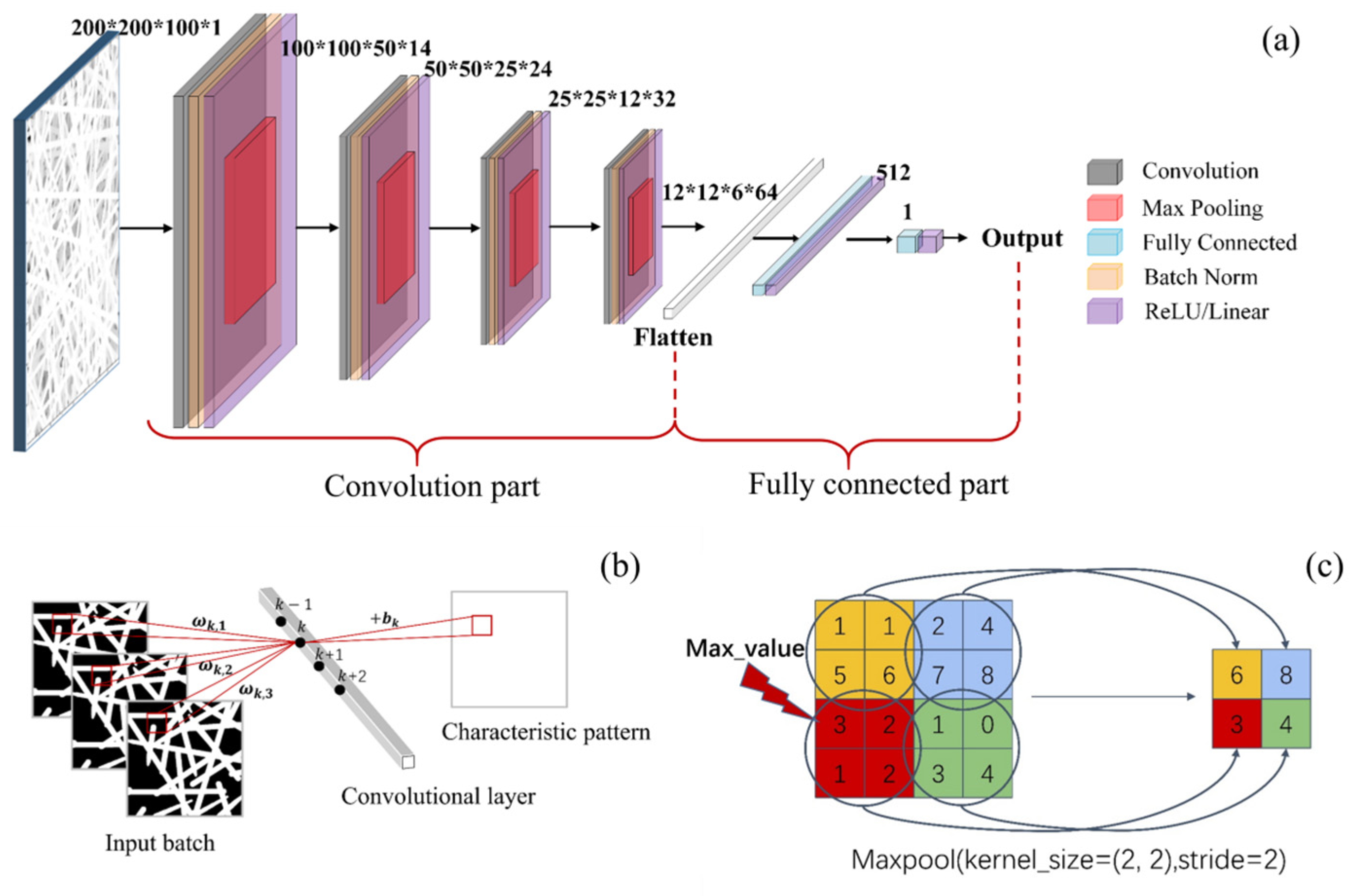
CNN [31] is a widely used deep learning algorithm for tasks such as image recognition, image classification, and image regression [43,59]. A CNN consists of convolutional layers, pooling layers, and fully connected layers. As shown in Figure 6a, a CNN can be viewed as comprising convolutional components and fully connected layers, where the fully connected layers function similarly to a simple ANN, accepting the data output from the convolutional layers and employing multiple layers of neurons for learning. As depicted in Figure 6b, within a CNN, the convolutional layers perform convolution operations on the input images, with the formula referenced in Equation (20) [59]:
z i , j , k l = w k l T · x i , j l + b k l
where z i , j , k l is the value at (i, j) in the k-th feature map of the l-th layer, w k l and b k l are the weight vector and bias term of the k-th convolution kernel of the l-th layer, respectively, and x i , j l is the input group located in the l-th layer with the center position at (i, j). After processing the results through an activation function, pooling operations are performed on the output to reduce the number of parameters and computational load in the subsequent layers of the model [60,61,62]. Typical pooling operations include max pooling and average pooling, with the formulas referenced in Equation (21) [43,59].
y i , j , k l = p o o l ( a m , n , k l ) , ( m , n ) n i , j
where y i , j l is the value at (i, j) on layer l, feature map k after pooling operation. a m , n , k l is the pooling region containing the set of locations ( m , n ) on layer l, feature map k, and n i , j is the region near (i, j) before the pooling operation.
In CNN, max pooling is frequently used. As shown in Figure 6c, the pooling kernel scans the pooling region and assigns the maximum value within that region to the pixel at the corresponding position in the new feature map. The strengths of CNN in processing images and multidimensional data have led to its application and research in estimating the spatial thermal properties of batteries and battery states.
Mengyi Wang et al. [63] combined a CNN model with Virtual Thermal Sensor (VTS) technology to obtain internal battery temperatures without the need for any thermal characteristics, heat generation, or thermal boundary conditions of the battery solely by measuring external battery temperatures. The measured external temperatures were presented as an 8 * 8 thermal map for input into the CNN, with the CNN outputting estimated values for 64 internal temperatures. Additionally, the CNN’s predictions were compared with those of linear regression (LR). The model’s performance on the test set is shown in Table 1. The CNN outperforms LR in terms of goodness of fit (R2), MAE, and MSE, showing a clear advantage in temperature prediction accuracy. Moreover, the CNN prediction time is 1.49 s (<5 s), which makes it possible to predict and monitor the internal temperature of the battery in real time by CNN combined with VTS only through external temperature.
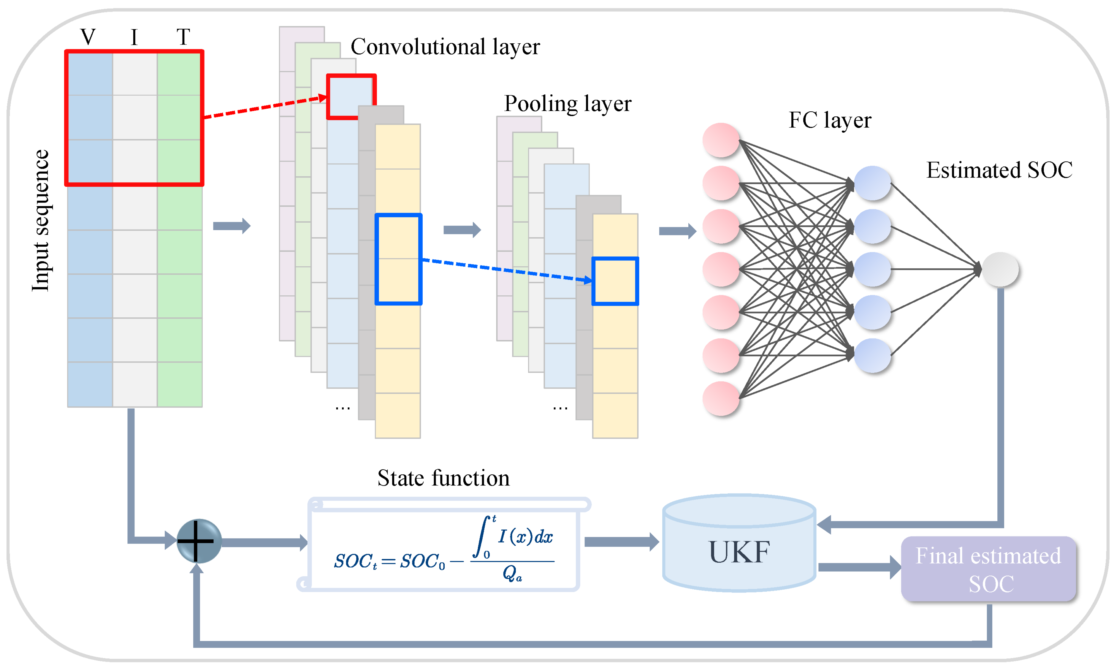
To harness the full potential of CNN and expand its capabilities, some studies have successfully combined CNN with other algorithms for efficient prediction of battery characteristics. Hongli Ma et al. [64] employed a hybrid approach that integrates CNN with the Unscented Kalman Filter (UKF). As shown in Figure 7, without the need for complex internal chemical reaction information of the battery, the measured voltage, current, and temperature of the LIB served as input data for the CNN, which extracted the time series features of the input data and corrected using UKF to output high-precision SOC estimation. Additionally, the study compared the performance of this model with simple CNN and other advanced methods under different temperatures and conditions, showing that the CNN-UKF method outperforms other data-driven SOC estimation methods in terms of accuracy and robustness, with the average values of RMSE and MAE also significantly reduced, up to 61.50% and 69.27% improvement. This method eliminates the need for manual tuning of CNN network hyperparameters, reduces the model’s sensitivity to hyperparameters, improves network efficiency, and demonstrates excellent performance in enhancing the model’s accuracy and robustness.
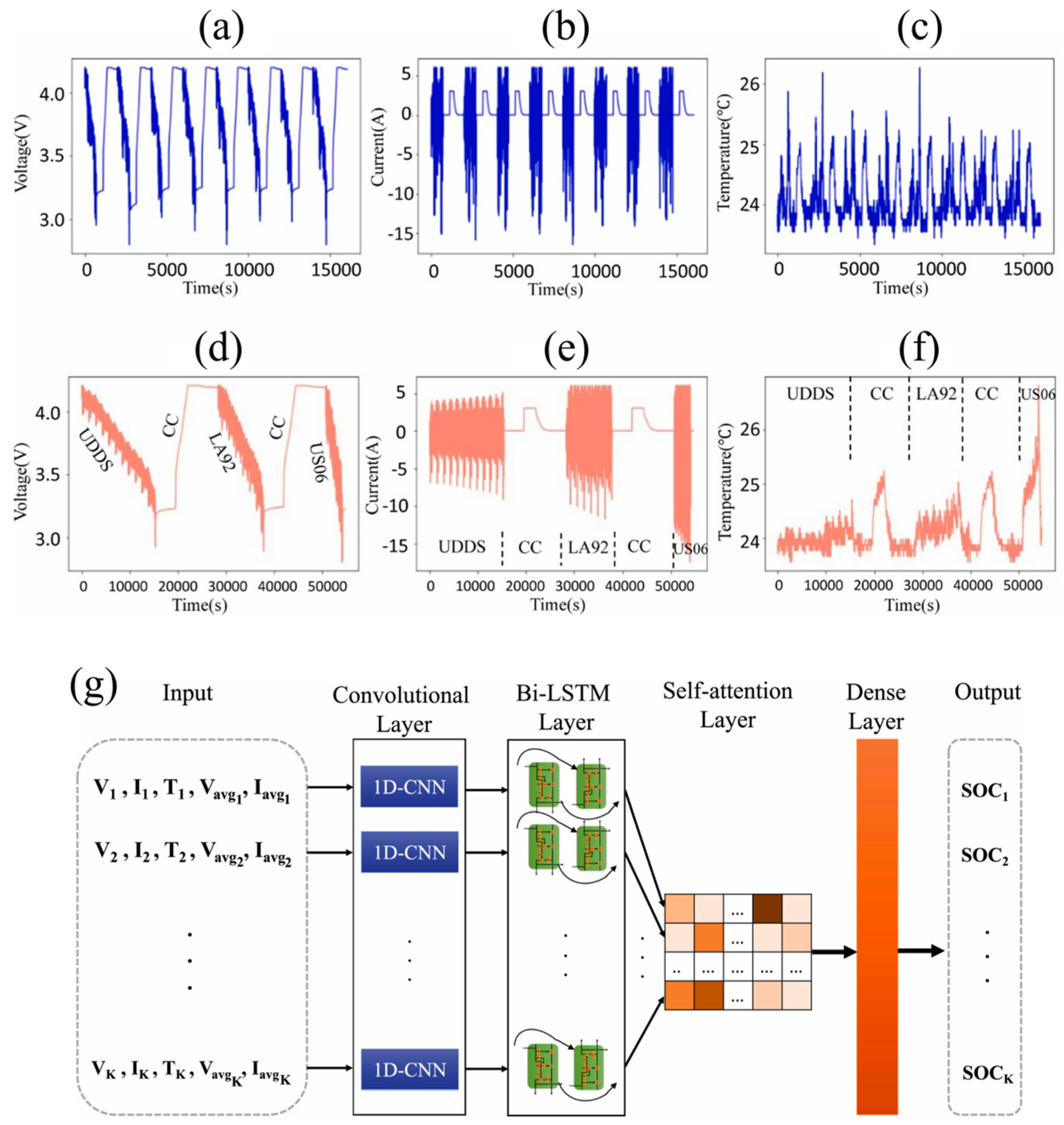
Although significant accuracy in SOC estimation has been achieved at room temperature using deep learning algorithms, SOC estimation at lower temperatures still requires more complex network architectures to capture the intricate features affecting battery dynamics. To accurately estimate SOC at lower temperatures, Zeinab Sherkatghanad et al. [65] proposed a robust deep learning model based on CNN (CNN-Bi-LSTM-AM), which can effectively generalize across a wide range of ambient temperatures, addressing the challenge of achieving precise SOC estimation over a broad temperature range. As shown in Figure 8g, the model integrates a self-attention mechanism, CNN, and Bidirectional Long Short-Term Memory (Bi-LSTM) network, effectively processing the inherent spatial and temporal information of lithium-ion battery data. As depicted in Figure 8a–f, the study utilized 160,453 datasets from mixed drive cycles as the training dataset and 54,727 datasets from automotive industry standard driving cycles as the test set. The model takes current, voltage, temperature, average current, and average voltage as inputs and outputs SOC prediction values. The model was validated by comparing the SOC estimation results at room temperature (25 °C) and three lower ambient temperatures (10 °C, 0 °C, −10 °C) using 12 different deep learning models (including LSTM, Bi-LSTM, CNN-LSTM, with and without attention mechanism). The results, as shown in Table 2, demonstrate that the CNN-Bi-LSTM-AM model proposed in this study exhibits high estimation accuracy and predictive performance across different temperature conditions. Deep learning models that combine multiple techniques often show a more powerful generalization ability and excellent performance.
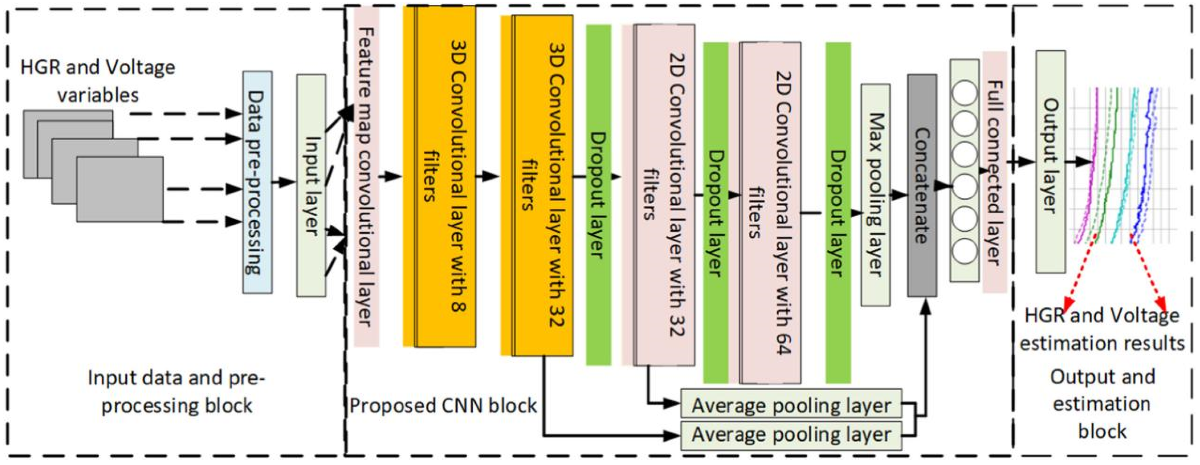
In addition to battery temperature and state, accurate estimation of battery heat generation rate (HGR) and voltage is crucial for the safe and efficient operation of electric vehicle BTMS. To estimate and optimize the thermal generation rate and voltage distribution of lithium-ion batteries for application in electric vehicles, S. Yalçın et al. [66] proposed a model named CNN-ABC. As shown in Figure 9, this model combines the advantages of CNN with the Artificial Bee Colony (ABC) optimization algorithm. It captures hidden features in the data through CNN and optimizes HGR and voltage estimation using the ABC algorithm. Additionally, the study compared the proposed model with other AI methods, showing that the CNN-ABC model outperformed other AI methods in both HGR and voltage estimation, with an HGR estimation RMSE of 1.38% and R2 of 99.72% and a voltage estimation RMSE of 3.55% and R2 of 99.82%. The study shows that CNN combined with ABC can better solve the problem of accurate estimation of battery HGR and voltage.

3.2. Residual Neural Network (ResNet)

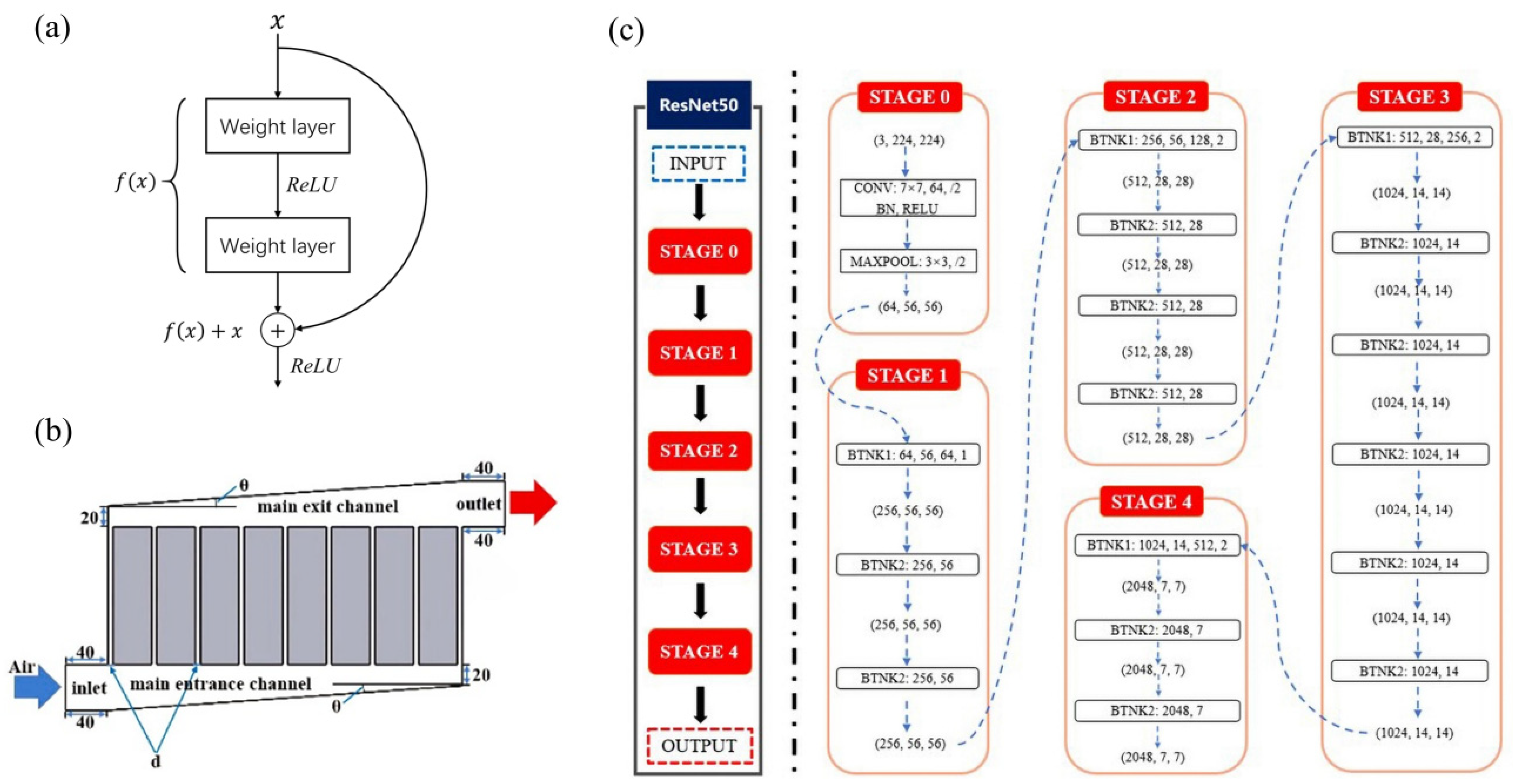
ResNet [67] is a deep learning algorithm that improves upon the CNN architecture, as shown in Figure 10a. By integrating residual modules into the CNN, it allows signals within the network to bypass one or more layers, directly propagating from input to output. This effectively mitigates common issues such as vanishing and exploding gradients, as well as the performance degradation often encountered during the training of deep network (where the model’s effectiveness decreases with the addition of more layers). Consequently, ResNet enhances the training efficiency and stability of deep learning models. Currently, ResNet has found applications in complex feature recognition and deep network problems.
In the research by Yuan Xu et al. [30], a method based on fluid dynamics and ResNet was proposed to optimize the thermal management and aerodynamic noise performance of a marine power battery air-cooling BTMS. As shown in Figure 10b, the study used a single battery module containing eight identical LFP (LiFePO4) marine batteries, equipped with a Z-shaped layout BTMS. Room temperature ambient air enters through the inlet channel at the lower left of the module, with cooling channels uniformly distributed at intervals of d. The study investigated the impact of system structural parameters and operational parameters, such as battery spacing (d), main channel inclination angle (θ), and inlet velocity (v), on thermal management performance (maximum temperature Tmax and maximum temperature difference ΔTmax) and aerodynamic noise performance (overall sound pressure level OSPL). As shown in Figure 10c, the study employed the ResNet-50 model to establish the relationship between system parameters and performance indicators, achieving rapid and accurate prediction. By inputting battery spacing (d), main channel inclination angle (θ), and system inlet velocity (v), the model fits and outputs Tmax, ΔTmax, and OSPL through the ResNet-50. Furthermore, the study combined ResNet-50 with the TOPSIS evaluation method to determine the optimal system structure and operational parameters. The results showed that, compared to the baseline, the optimal case reduced the maximum temperature by 10.63 K and the maximum temperature difference by 9.41 K. At the same time, under the best operational parameters in the prediction set, the model’s maximum temperature error was 0.08%, and the maximum temperature difference error was 2.64%, which shows that the use of ResNet to judge the performance of BTMS is almost the same as that of the simulation method, and the use of deep learning technology can significantly save the computational cost and help to accelerate the determination of the best working condition parameters.
In the research by Xin Cao et al. [68], an early diagnosis method for overcharge thermal runaway based on the Gramian Angular Summation Field (GASF) [69] and the residual network (ResNet) was proposed. As shown in Figure 11, the study obtained surface temperature data of lithium-ion batteries (lithium iron phosphate) during normal and overcharge processes through experiments and divided them into different stages (normal charge, early overcharge, and middle overcharge). GASF was used to convert the measured surface temperature time series into two-dimensional thermodynamic images, where pixel values represent temperature levels. The ResNet18 model was employed to extract features from thermodynamic images, enabling the classification of the three states. This method can achieve a diagnostic accuracy rate of 97.7% before the battery surface temperature reaches 50 °C, realizing early warning and safety monitoring for lithium-ion battery overcharge thermal runaway. Additionally, the method was tested on 12 Ah and 20 Ah lithium iron phosphate batteries, demonstrating good reliability and applicability. The research shows that ResNet can extract features from battery surface temperature data, enabling early diagnosis of overcharge thermal runaway and enhancing the safety and reliability of lithium-ion batteries.

3.3. Recurrent Neural Network (RNN)

In predicting battery thermal properties and states, the SOC curve, voltage curve, temperature curve, and other time series fluctuate over time and often exhibit strong autocorrelation. Traditional deep neural network extends longitudinally, improving learning effects by increasing the number of neuron layers, but this approach does not consider the temporal changes in each hidden layer. Although CNN can extract features from time series through convolution operations, these operations focus on the features of nearby sequences. When a larger time interval separates two features, multiple layers of convolution operations are often required to associate the two features, greatly increasing the network’s complexity and computational load.
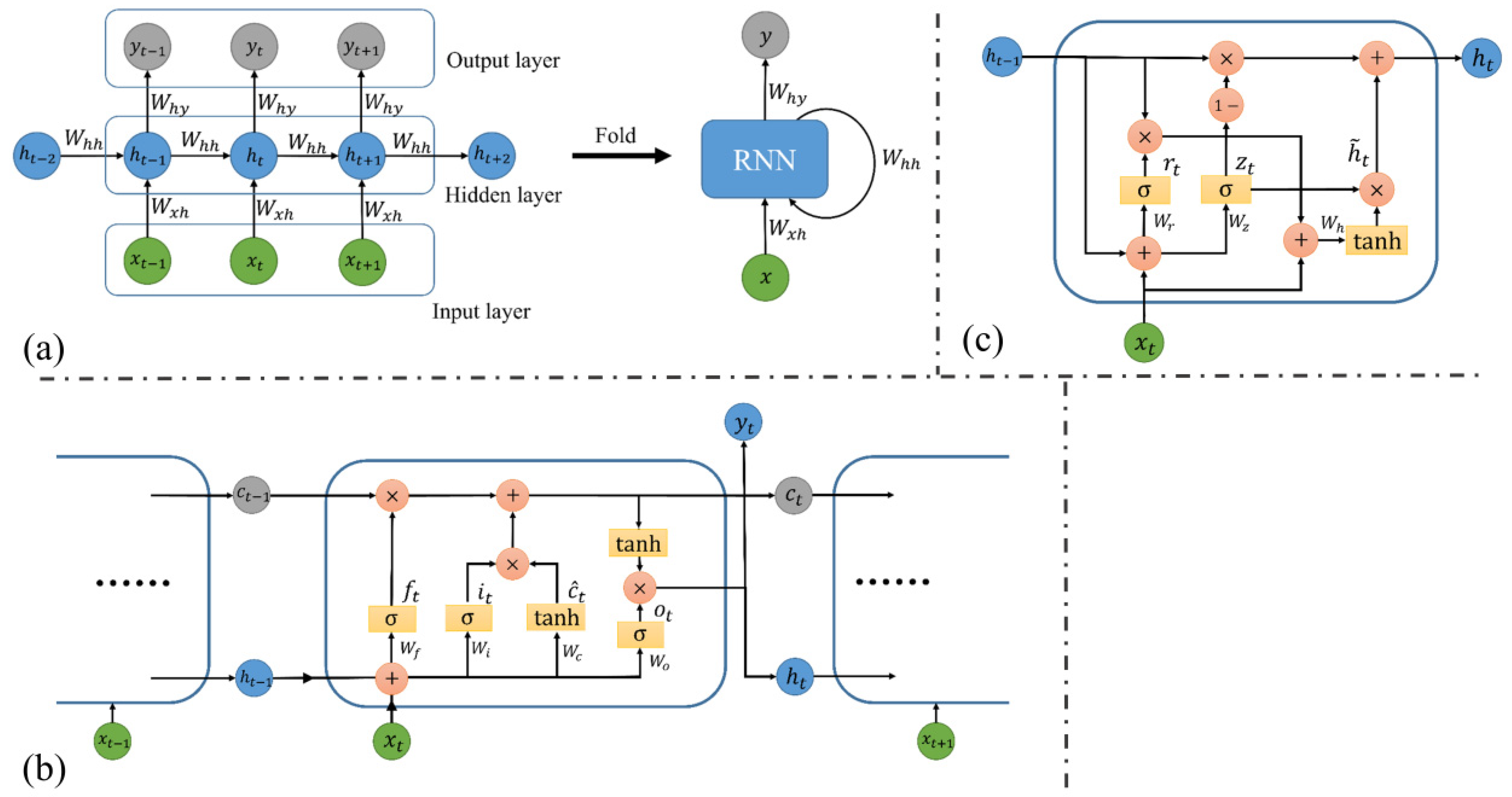
A Recurrent Neural Network (RNN) [70] is a deep learning algorithm for processing sequential information, introducing relationships between preceding and subsequent time steps in a neural network. An RNN mainly consists of input layers, hidden layers, and output layers [8]. As shown in Figure 12a, the hidden layer of an RNN processes the input of a sequence element one at a time and uses the output of the hidden layer as additional input for the next sequence element [71,72]. The RNN retains the influence of the previous sequence features on the current sequence features. The output y t of RNN at the current time t is referred to in Equations (22) and (23) [72,73], where f is the activation function, x 1 x n is the input sequence, h t is the hidden state at that instant, W x h , W h h , W h y is the weight, and b h , b y is the bias.
h t = f ( W x h x t + W h h h t 1 + b h )
y t = W h y h t + b y
Although RNN has strong capabilities for processing time series problems, it often struggles to capture features from earlier sequences as the number of time steps increases. The LSTM [32] is an improved algorithm based on RNN, addressing the issue of traditional RNN having only short-term memory and being unable to handle longer time series [8]. Moreover, LSTM also resolves the issues of training instability caused by gradient explosion and vanishing gradients in RNN [74]. As shown in Figure 12b, LSTM handles long-term dependencies through its input gate, output gate, and forget gate, with these three gates using a sigmoid function (ranging between 0 and 1) to determine how much past information is remembered and how much new information is forgotten in the current cell [75,76]. The specific operations are detailed in Equations (24)–(29) [76,77]:
i t = σ ( W x i x t + W h i h t 1 + b i )
f t = σ ( W x f x t + W h f h t 1 + b f )
c t = tanh ( W x c x t + W h c h t 1 + b c )
c t = f t · c t 1 + i t · c t
o t = σ ( W x o x t + W h o h t 1 + b o )
h t = o t · tanh ( c t )
where c t is the updated state output of the unit; i t , f t and o t denote the input gate, forget gate, and output gate, respectively. σ is the activation function (sigmoid function), W and b denote the associated weights and biases. Compared with the traditional RNN, its hidden layer is no longer a simple temporal superposition, but considers the interaction of multiple gates. To understand LSTM better, it is necessary to think more closely about human neurons. In LSTM, c t 1 can be regarded as the memory of the previous moment, the forgetting gate f t determines the proportion of forgotten c t 1 in the unit at this moment, and c t can be regarded as the new memory generated in the unit at this moment. It is determined by the hidden state h t 1 of the unit at the previous moment and the input x t at this moment. The input gate i t determines how many new memories will be saved at this moment. The new memory is superimposed with the previous memory to output the memory c t at this moment. At the same time, the hidden state h t of the unit at this time is jointly affected by the memory c t at this time, the hidden state h t 1 at the previous time, and the input x t at this time.
While LSTM can handle longer time series and capture key information through its complex computational mechanisms, the introduction of multiple gates makes the network structure more complex, increasing the computational cost [8,78]. To address the increased computational load caused by parameter redundancy in LSTM, a less computationally intensive gated RNN, known as the GRU [33,77,79], was designed. The GRU model performs similarly to the LSTM but has a simpler structure with fewer network parameters, leading to faster training speeds [71,73,80]. As shown in Figure 12c, the GRU consists of a reset gate and an update gate. The reset gate influences the extent to which the memory from the previous moment is retained, while the update gate filters new memories and determines which memories are preserved and propagated to the next moment. Its operations are detailed in Equations (30)–(33), as follows:
r t = σ ( W x r x t + W h r h t 1 + b r )
z t = σ ( W x z x t + W h z h t 1 + b z )
h t ~ = tanh ( W x h x t + W h ( r t · h t 1 ) + b h )
h t = ( 1 z t ) · h t 1 + z t · h t ~
LSTM and GRU control the flow of information from one moment to the next through gating mechanisms, addressing the challenges of capturing long-term dependencies and the issues of gradient explosion and vanishing gradients faced by traditional RNN. In the context of battery thermal management applications, LSTM and GRU are widely utilized to learn sequences that encompass temporal information, such as temperature, voltage, and SOC (State of Charge). They have been correspondingly researched for applications in battery thermal early warning systems and temperature monitoring.
In the study by Zhenhua Cui et al. [80], a neural network model combining CNN and bidirectional weighted gated recurrent unit, known as CNN-BWGRU, was proposed to address the issue of decreased accuracy in SOC estimation for lithium-ion batteries in low temperature environments. This model aims to accurately and stably estimate the SOC of lithium-ion batteries under low temperature conditions, ensuring the safety and stable operation of the batteries. As shown in Figure 13, the study introduced a “multi-moment input” structure to optimize the impact of battery information on estimation results, thereby strengthening the connection between output and input and enhancing the overall network performance. As shown in Table 3, the proposed CNN-BWGRU model achieved excellent estimation performance, with an MAE and Root Mean Square Error (RMSE) of less than 0.0127 and 0.0171, respectively. Compared with the traditional GRU and CNN-GRU models, CNN-BWGRU has higher accuracy, robustness, and generalization ability in the estimation of SOC of lithium-ion batteries under low temperature conditions.
In the study by Siyi Tao et al. [77], the performance of different RNN models (LSTM, GRU, Bidirectional GRU (BGRU), and Bidirectional LSTM (BLSTM)) in estimating the SOC of electric vehicle lithium-ion batteries was compared under three different test cycles (NEDC, UDDS, and WLTP). The study used a dataset from experiments conducted on commercial 18,650-type batteries, which included data on battery current, voltage, and SOC values for training the four models. The results showed that the BLSTM model performed the best under NEDC, UDDS, and WLTP conditions, with MAE values of 1.05%, 7.81%, and 1.81%, respectively. s
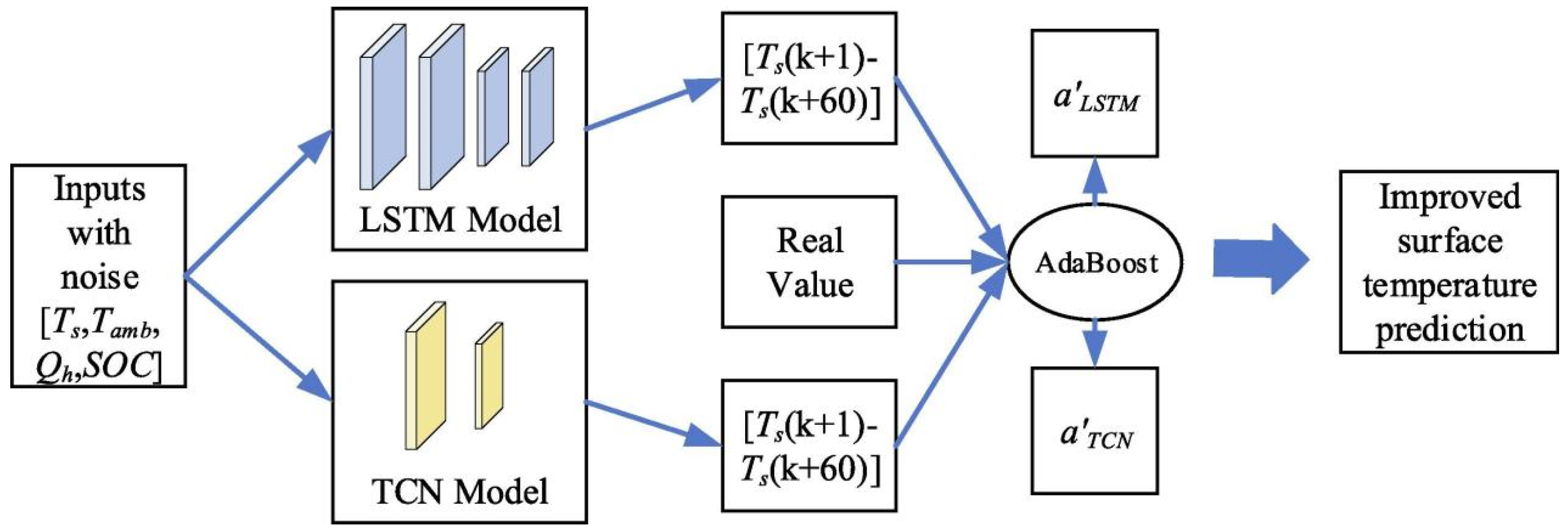
In battery thermal management, temperature has a significant impact on the safety and performance of batteries. Therefore, predicting the temperature trends of lithium-ion batteries and implementing early warning systems for abnormal heat is crucial. Marui Li et al. [81] proposed a battery thermal early warning system named the Sequential-Transformer Thermal Early Warning System (STTEWS). As shown in Figure 14, a model combining CNN and LSTM, known as TCRDN, was used to estimate temperature trends for the early warning system. The TCRDN can use a 20-s time series to predict changes in the surface temperature of the lithium-ion energy system for the next 60 s. Additionally, the study compared the performance of this model with LSTM and TCN in predicting surface temperature. The results indicated that TCRDN, combining the advantages of LSTM and TCN, achieved more accurate predictions for lithium-ion batteries. Compared to TCN, the MSE of TCRDN was reduced by up to 0.01; compared to LSTM, the reduction could reach 0.02. TCRDN can effectively predict battery thermal runaway 1 min in advance, which makes this method more practical in the development of BTMS and ensuring battery thermal safety.
Safieh Bamati et al. [82] proposed a sensorless battery temperature estimation method based on LSTM and DNN for estimating the surface temperature of cylindrical lithium-ion batteries. The study used a time series of voltage and current, along with their averages, as input features, capturing the nonlinear characteristics of the time series through LSTM layers and further improving estimation accuracy through fully connected layers. The research demonstrated that the LSTM-DNN model could accurately estimate the surface temperature of the battery throughout the entire aging cycle, with a prediction error range of only 0.25–2.45 °C. Because no contact sensor is needed, the problems of slow response speed, low sensitivity, and poor stability caused by direct temperature measurement are successfully solved, and it shows higher prediction accuracy in the later cycle of the battery.
Qi Yao et al. [83] employed GRU with an improved data normalization method to estimate the surface temperature of lithium-ion batteries. The model predicted the time series of battery surface temperature by inputting the time series of voltage, current, SOC, and ambient temperature. The GRU model demonstrated exemplary performance and generalization capabilities under different ambient temperature conditions and various driving cycles. Under fixed ambient temperature conditions, the MAE was less than 0.2 °C, and under varying ambient temperature conditions, the MAE was less than 0.42 °C, which is significant for battery thermal management and safety assessment. Under the premise of ensuring the accuracy of temperature prediction, this method does not rely on any physical battery model or filter, which reduces the complexity of modeling and effectively alleviates the demand pressure of the number of temperature sensors and the rising cost.
Da Li et al. [84] proposed a battery thermal runaway prediction model. This model requires the calculation of the battery’s heat generation rate based on the trends in battery temperature, external ambient temperature, and the state of the battery to determine whether abnormal heat generation has occurred and thus predict thermal runaway. In the battery temperature prediction, a model combining LSTM and CNN was used. CNN was employed to extract spatial features from the input data, while LSTM extracted temporal sequence features, combining the two to better predict the spatial and temporal temperature characteristics of the battery. To reduce computation time, the authors used Principal Component Analysis (PCA) to compress the input factors and the Random Approximation Optimization Method (RAOM) to automatically optimize the model’s hyperparameters. After thorough training, the model can accurately predict the battery temperature for the next 8 min with an average relative error of 0.28%, and the battery thermal runaway can be accurately judged 27 min in advance. The proposed model provides an effective means for early warning of thermal runaway failure of batteries under diverse and changing driving conditions.

3.4. Generative Adversarial Neural Networks (GAN)

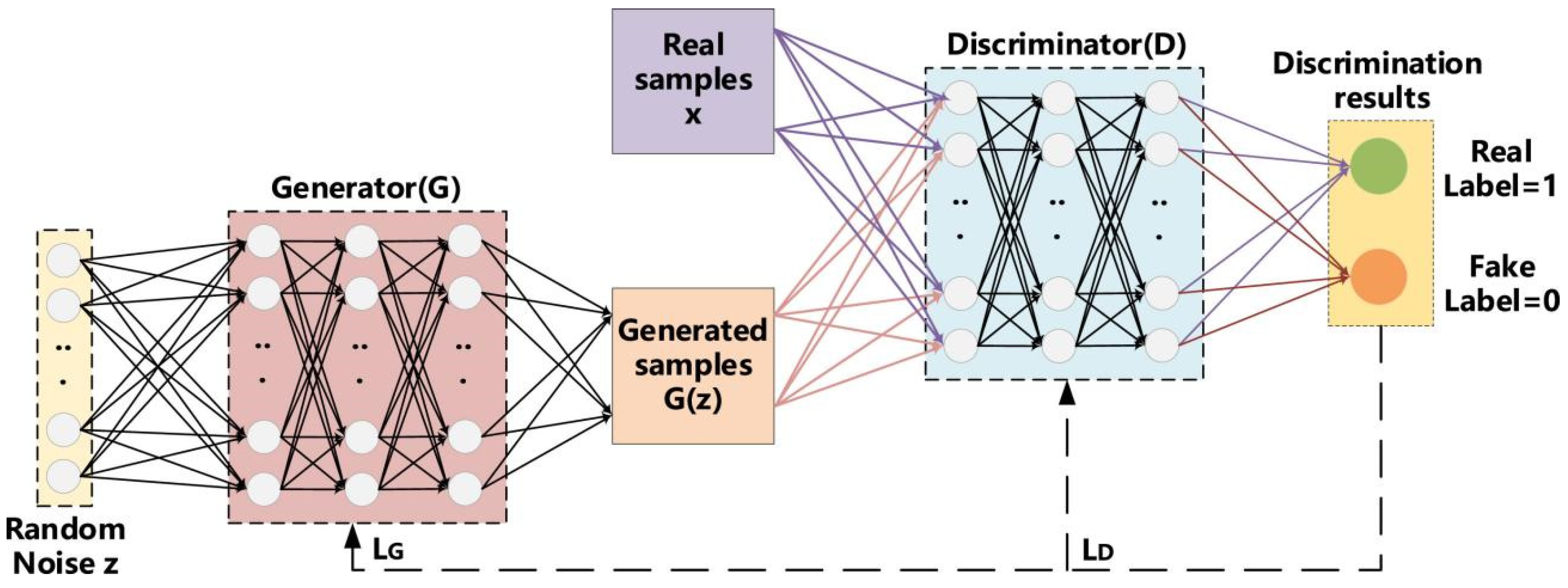
Currently, to ensure the effectiveness of deep learning, a large amount of training data is required. For instance, estimating the SOC of a battery necessitates a substantial amount of carefully selected battery parameter data (such as voltage, current, and temperature). Collecting data through repeated experiments incurs high costs and time, and the lack of diversity in publicly available datasets limits research in this field [85]. The GAN [34], proposed by I. Goodfellow et al. in 2014, is a deep learning algorithm that has achieved significant success in applications such as data generation and image style transfer [86,87,88]. In the prediction of battery properties and the design of BTMS, GAN can be utilized to expand sparse datasets, addressing the challenges of data acquisition and the issue of data uniformity. This approach can enhance the learning capacity and robustness of predictive models. As shown in Figure 15, this deep learning model consists of two main parts: the generator and the discriminator. The generator’s goal is to learn the distribution of real samples x and to generate synthetic samples G (z) that are similar in dimension to the real samples. The generator’s input is random noise z that follows a simple distribution, which is processed through multiple layers of neural networks to ultimately produce the synthetic sample G (z). The discriminator’s purpose is to accurately distinguish between x and G (z) by extracting features from the input samples and outputting a judgment result. During the training of the discriminator, when the input is x, the expected judgment result is Real (Label = 1), and when the input is G (z), the expected judgment result is Fake (Label = 0). The optimizer then optimizes the discriminator’s parameters based on the loss LD. When training the generator, the loss LG is the error between the output of the discriminator judging the samples generated by the generator and Label = 1. The optimizer optimizes the generator’s parameters through LG, causing the generator’s output features to increasingly resemble those of real samples. There is a competitive and adversarial relationship between the generator and discriminator, with the generator continuously optimizing to pass the discriminator’s judgment, while the discriminator must be constantly trained to correctly distinguish between generated and real samples [86,89]. In GAN training, binary cross-entropy (BCE) is often used as the loss function to optimize the model, steering the generator towards the direction where the discriminator’s correct judgment probability is minimized, while the discriminator is optimized to maximize the correct judgment probability. This is referenced in Equation (34) [86]:
min G max D V ( G , D ) = E x ~ P d a t a ( x ) [ log D ( x ) ] + E z ~ P z ( z ) [ log ( 1 D ( G ( z ) ) ) ]
where V ( G , D ) is the binary cross-entropy loss, when training the generator, it is to minimize the loss ( min G V ( G , D ) ) or to maximize the loss ( max D V ( G , D ) ), E [ ] is the expected value of the sample distribution function, x, P d a t a ( x ) represents the actual sample and the actual sample distribution, z, P z ( z ) represents random noise input to the generator and the distribution of the noise, and G ( z ) is the sample generated by the generator. D ( x ) is the probability that the discriminator determines that x is from the real sample, and D ( G ( z ) ) is the probability that the discriminator determines that G ( z ) is a real sample.
In the research by Falak Naaz et al. [85], a data augmentation method based on GAN was proposed. This method utilizes a Time Series GAN to generate synthetic battery parameter data, such as voltage, current, temperature, and SOC, thereby expanding sparse datasets and enhancing the learning capabilities of neural networks used for SOC estimation. The method was evaluated on two publicly available battery parameter datasets (Oxford battery degradation and NASA prognostics data repository), achieving Kullback-Leibler (KL) divergence values of 0.2317 and 1.0572, respectively. The results indicate that the model-generated data possess a high degree of fidelity, addressing the lack of diversity and labeling in battery parameter datasets and removing a fundamental obstacle in SOC estimation research.
Additionally, in the research by Xianghui Qiu et al. [90], which also targeted the issue of limited training data for data-driven SOC estimation models, a CGAN model was employed, combined with LSTM to capture the temporal characteristics of battery dynamic cycling data. The CGAN generated high-fidelity battery data sequences under specific conditions to enhance model training. Compared to regular GAN, the generator of a CGAN not only maps from random noise to output features but also maps from provided supplementary information to output features. The proposed model in the study can not only capture the temporal characteristics of battery data but also generate conditional data based on external factors such as temperature. Training a standard LSTM with both synthetic and real data to estimate SOC achieved an accuracy with an MAE of less than 0.5% and an RMSE of less than 1%. Compared to training solely with real data, the use of a mixture of synthetic and real data for training significantly improves the performance of the SOC estimation model.
Currently, thermal runaway of onboard power batteries is a key issue affecting their safety and is a major focus that BTMS strives to address. However, the long upload cycle of cloud systems in electric vehicles—typically around 10 s—makes it challenging to construct regression models capable of accurately predicting abnormal battery states. Reconstruction-based methods have emerged as a promising approach for predicting the thermal runaway of lithium-ion batteries [91]. The data generation capability of GAN has found some application in these reconstruction-based methods for predicting lithium-ion battery thermal runaway.
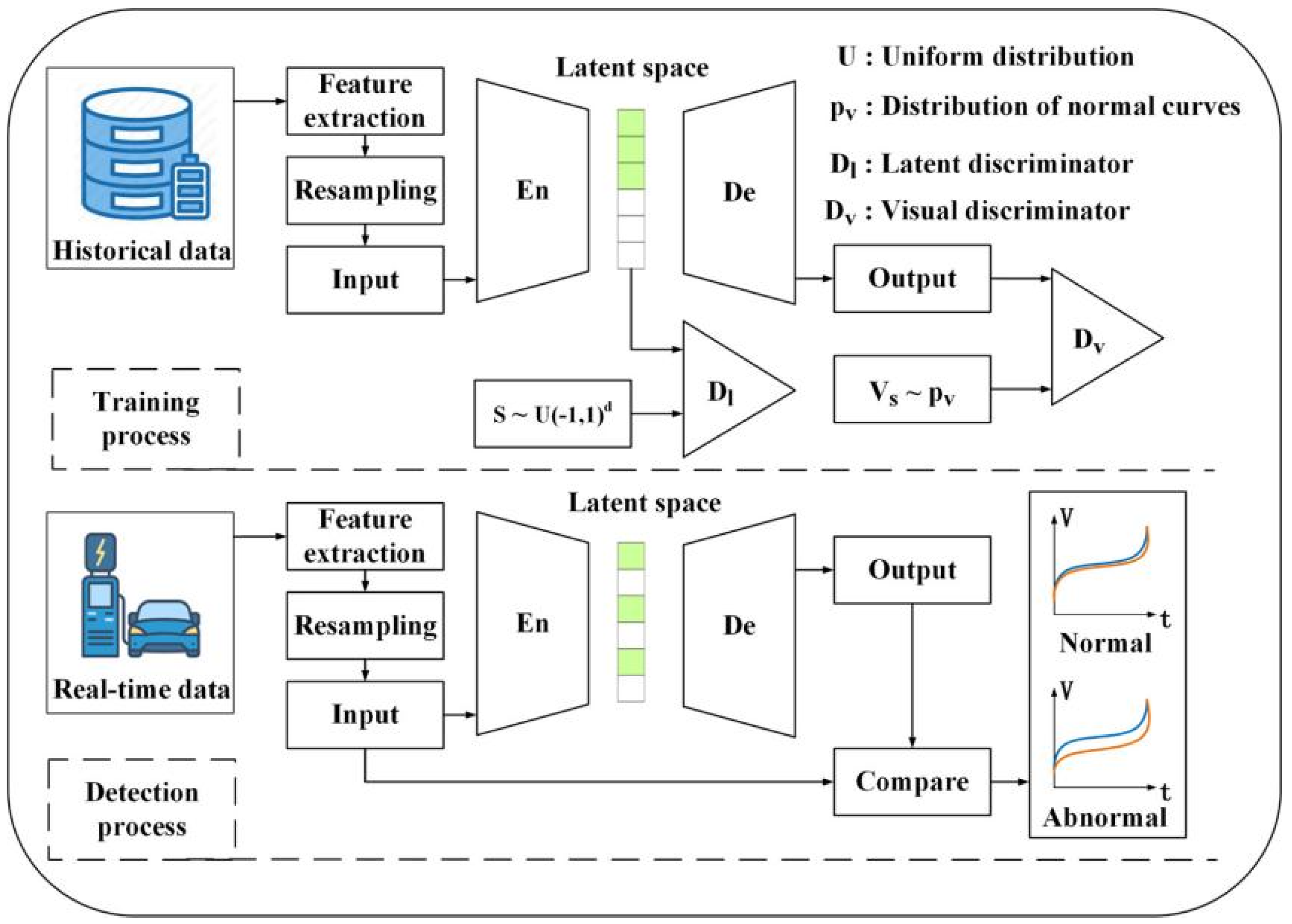
In the research by Heng Li et al. [91], a GAN-based method for predicting the thermal runaway of lithium-ion batteries was proposed. As shown in Figure 16, this method leverages GAN to generate a detection model that provides a reference normal charging voltage curve for the original battery charging process, thereby detecting potential abnormalities. Through training, the generator is ensured to output only normal charging curves. In actual detection, the presence of an abnormal state is determined by comparing the reconstruction error between the reference curve generated by the generator and the actual curve. The study compared the performance of the proposed method with other methods, and the experimental results show that GAN can accurately identify all abnormal batteries before thermal control occurs and reduce the false positive rate to 1.75%. Compared with the 3σ method, LOF method, and autoencoder method, the false positive rate is reduced by 31.18% at most, which is significantly better than some existing methods.
In battery thermal management, temperature is a key indicator for assessing the state of lithium-ion batteries and preventing thermal runaway. When estimating battery temperature through thermal images, a large number of diverse images are needed to ensure good model training. However, obtaining thermal imaging samples of lithium-ion batteries can be difficult due to high experimental costs and associated risks [92]. The data generation capability of GAN has also been applied to expand the limited data on battery temperature thermographs.
As shown in Figure 17, in the research by Fengshuo Hu et al. [92], a method based on CGAN and ResNet was proposed for expanding the dataset of lithium-ion battery fault thermographs. To address the issue of gradient disappearance and mode collapse in GAN caused by using the Jensen-Shannon (JS) divergence as the generator’s loss function and to increase training stability, the study employed the WGAN-GP architecture, which replaces the traditional GAN’s generator loss function with the Wasserstein distance [93] and incorporates gradient penalty to enhance the convergence rate of the WGAN. The JS divergence is a modification of the Kullback-Leibler (KL) divergence that addresses its issue of asymmetry.
K L ( p q ) = x p ( x ) log p ( x ) q ( x )
J S ( p , q ) = 1 2 K L ( p p + q 2 ) + 1 2 K L ( q p + q 2 )
Subsequently, the JS divergence can be expressed as follows:
J S ( p , q ) = 1 2 p ( x ) log ( p ( x ) p ( x ) + q ( x ) 2 ) + 1 2 q ( x ) log ( q ( x ) p ( x ) + q ( x ) 2 )
where p ( x ) is the distribution of real samples and q ( x ) is the distribution of generated samples. Although the hot JS divergence effectively solves the asymmetry problem of KL divergence, when the two distributions do not overlap at all, their JS divergence is 0, so that the gradient is 0, which leads to the inability to update the model. As shown in Equation (38), the Wasserstein distance measures the minimum average distance needed to move data from distribution p to distribution q, solving the vanishing gradient problem of JS divergence,
W ( p , q ) = inf γ ( p , q ) E ( x , y ) ~ γ [ x y ]
where p is the distribution of real data, q is the distribution of generated data, and ( p , q ) represents the set of joint distributions of distributions p and q. To address the issue of gradient disappearance in traditional GAN, the paper introduced residual blocks into the network; that is, using ResNet instead of traditional CNN as the discriminator. The study simulated thermal images of lithium-ion batteries during the charging process with commercial software FLUENT to obtain battery data. The results indicated that the fault diagnosis accuracy of the model was improved after data augmentation, with an average accuracy increase of 33.8% and an average recall increase of 31.9%, and the introduction of WGAN-GP and ResNet can effectively improve the quality of the generated images.
Table 4 displays the applications of research of deep learning in lithium battery BTMS.

4. Emerging Deep Learning Algorithms for Battery Thermal Management

In summary, current deep learning methods, such as CNN, ResNet, LSTM, GAN, and others, have been extensively applied to assist in the design of BTMS. They play a significant role in predicting battery thermal properties, battery states, and preventing battery thermal runaway. The rapid prediction and generalization characteristics of deep learning enable it to maintain high performance under a wide range of battery operating conditions. In recent years, novel and efficient deep learning algorithms have continued to emerge, and these methods have also been applied and validated in other fields.

4.1. Diffusion Model (DM)

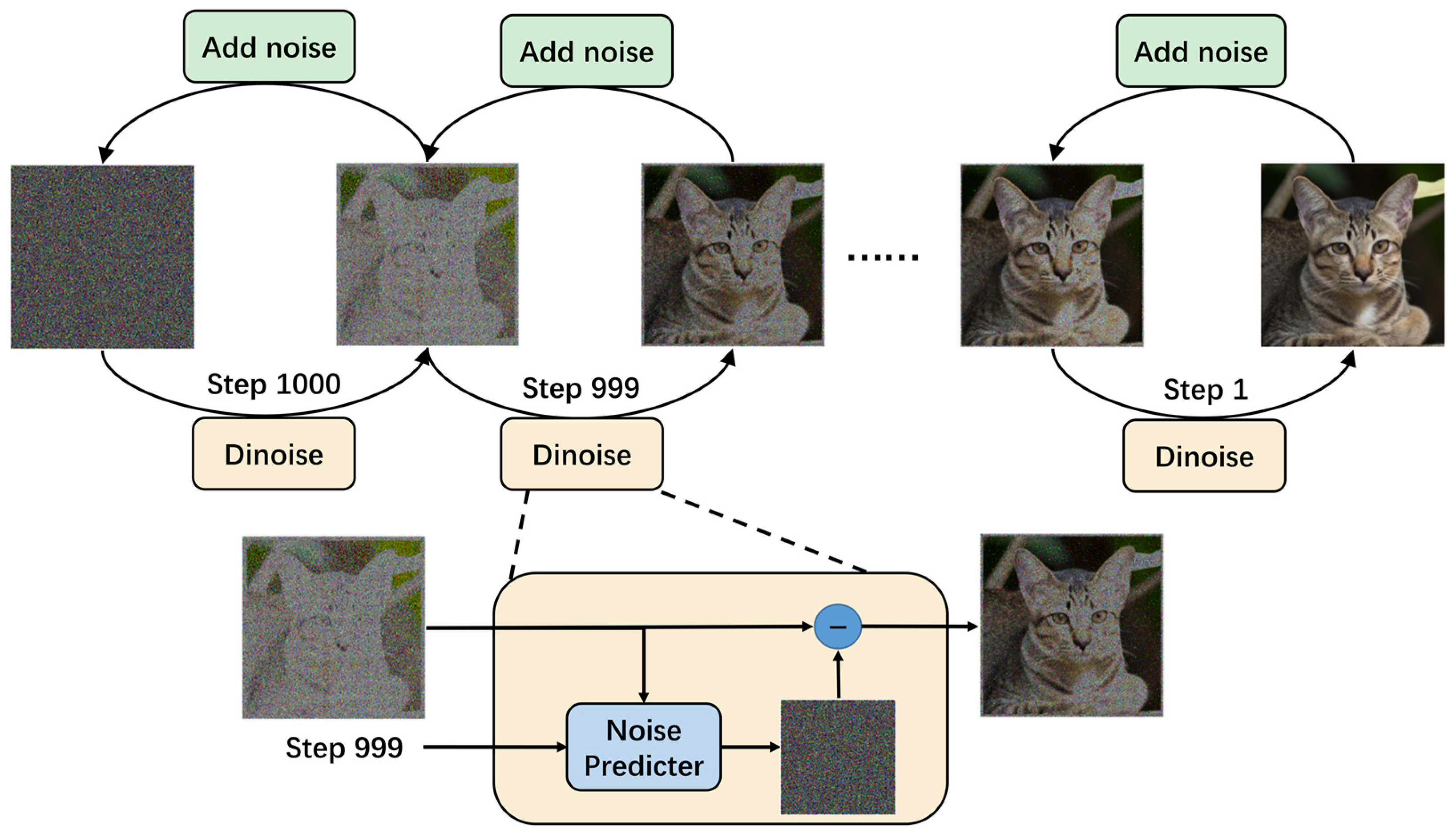
While GAN has achieved certain successes in data expansion and image generation, there are still some obstacles in its training. During the training of GAN, the generator’s training is affected by the discriminator’s performance. When the discriminator is too strong or too weak, it may cause the generator’s Mode Collapse (MC) and oscillation issues, making the model difficult to train and preventing the generation of diverse samples [94]. The proposal of DM has, to some extent, avoided these problems. DM is a powerful deep generative model that has shown significant performance in image synthesis, video generation, and molecular design, among other fields. Unlike GAN, DM does not rely on a discriminator to guide the generation process; it generates samples by progressively adding noise and learning the reverse process. DM offers better stability and has broken GAN’s long-standing dominance in image synthesis tasks, gradually gaining attention and application in recent years [95]. Currently, a widely used model in DM is the Denoising Diffusion Probabilistic Model (DDPM) [96]. Advanced text-to-image models such as OpenAI’s DALL·E 2 [97], StabilityAI’s Stable Diffusion [98], and Google’s Imagen [99] are all developed based on this. They utilize two Markov chains, one that gradually perturbs data into noise in the forward process and another that gradually denoises and converts noise back into data in the reverse process. As shown in Figure 18, in the forward process of DM, noise is introduced over multiple steps (typically set to 1000 steps) to corrupt and distort the data, with the image gradually losing its definition until it conforms to the desired distribution (usually a Gaussian distribution). The diffusion model learns the process of noise introduction at each step and uses a reverse transition kernel parameterized by a deep neural network to gradually reverse this diffusion process, allowing for the progressive denoising of the corrupted image and ultimately generating valid samples [95,100,101]. The forward and reverse processes of DM can be referenced in Equations (39)–(43) [100,101,102,103].
q ( x t | x t 1 ) = N ( x t ; 1 - β t x t 1 , β t I )
q ( x 1 , , x T | x 0 ) = t = 1 T q ( x t | x t 1 )
The original data x 0 ~ p ( x 0 ) , where q ( x t | x t 1 ) is the transition kernels, x 0 is the original data without noise, x 1 , , x T is the data after gradually adding noise, t stands for the number of steps of positive noise addition, T is the total number of steps, N ( ) stands for Gaussian distribution, I is the identity matrix, and β t ( 0 , 1 ) is the hyperparameter of transition kernels, are generally selected before training and then applied as follows:
q ( x t | x 0 ) = N ( x t ; i = 0 t ( 1 β i ) x 0 , ( 1 i = 0 t ( 1 β t ) ) I )
x t = i = 0 t ( 1 β i ) x 0 + 1 i = 0 t ( 1 β t ) z t
where z t N ( 0 , 1 ) . When t is large enough, i = 0 t ( 1 β i ) 0 , x t almost follows the Gaussian distribution N ( x t ; 0 , I ) . When generating new data, the DM generates a random noise vector from the prior distribution p θ ( x T ) = N ( x T ; 0 , I ) and uses a reverse transition kernel p θ ( x t - 1 | x t ) in the reverse Markov chain to gradually eliminate the noise.
p θ ( x t - 1 | x t ) = N ( x t 1 ; μ θ ( x t , t ) , θ ( x t , t ) )
where θ is the deep learning parameter. The reverse transition kernel p θ ( x t - 1 | x t ) receives a noisy image x t and a time step t as input, takes the denoised image x t - 1 as output, and learns to predict the mean μ θ ( x t , t ) and variance θ ( x t , t ) . By learning the operation of adding noise step by step and then performing the reverse operation, the noise was removed step by step, and, finally, x0, obeying the original data distribution, was obtained.
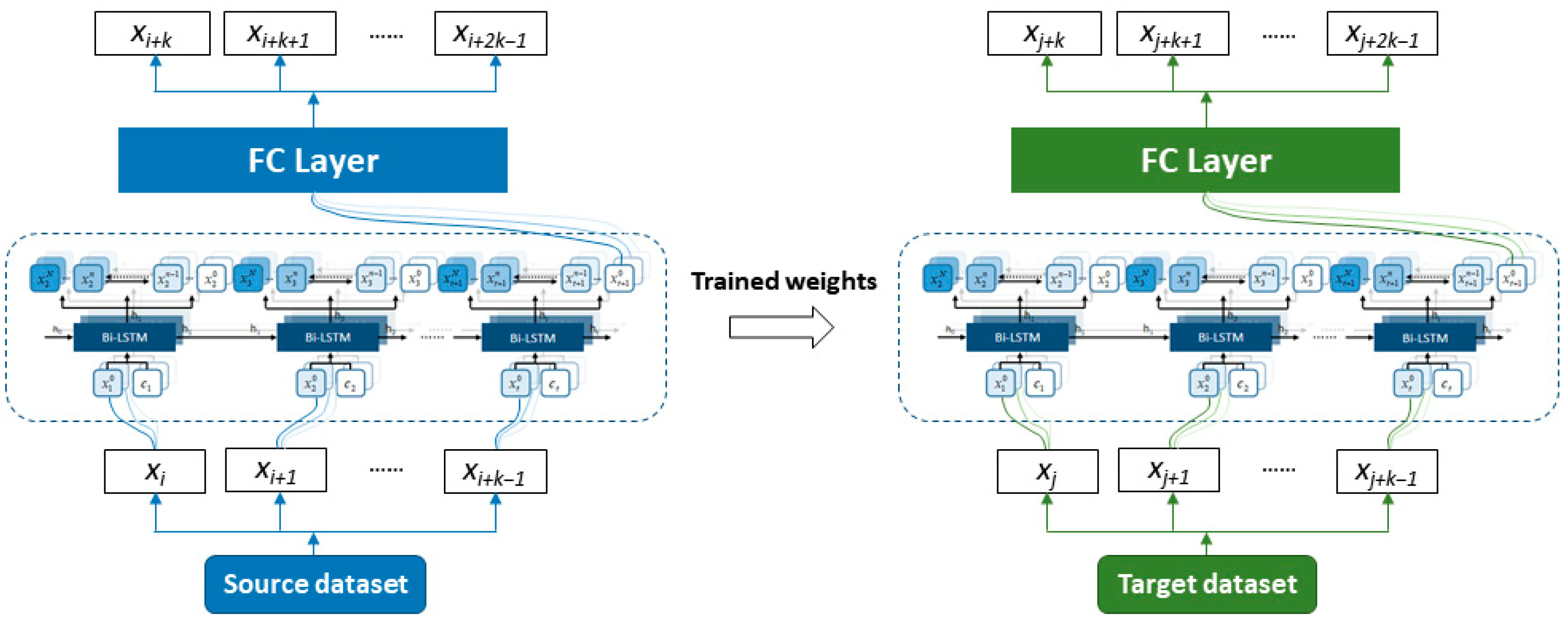
Currently, there is a lack of related research on the application of DM in BTMS, but in other directions, the ability of DM has been verified. Chenqiang Luo et al. [104] first applied DM to the research of LIB state health (SOH) prediction and proposed an SOH prediction model based on DM and Bi-LSTM combined with Transfer Learning technology. As shown in Figure 19, the study uses the voltage characteristics in the multi-stage fast charging process as input to predict the SOH of the battery through the reverse process of the DM. The model shows high accuracy and robustness on the source dataset, and the relative error is less than 4.5%. After transfer learning, the model still maintains high prediction performance, and the lowest RMSE, MAE, and MAPE can reach 0.0028, 0.0023, and 0.24%, respectively. The results show that DM can reduce the influence of data noise by learning the probability distribution of training data, the application of transfer learning reduces the dependence on labeled data in the target task, and the corresponding network model can be quickly built based on fewer data. At the same time, the method in this study can also be transferred to SOC prediction, which is helpful to develop less data-dependent battery monitoring models and realize efficient BTMS design in the future.
DM has also been successfully verified on a dataset with limited expansion. Tianrui Huang et al. [105] used DM to expand the limited training dataset successfully and used ResNet to realize the damage and defect monitoring of composite material structure, reaching an accuracy of 88.10%. DM possesses powerful image generation capabilities and offer better stability compared to GAN. However, the complexity of the model also increases the computational burden, and the numerous steps involved in the sampling process lead to slower model speeds [103], which is a significant barrier to the application of DM in the field of BTMS. Currently, DM is more suitable for tasks in BTMS design that require the expansion of datasets with high image quality demands, such as the generation of high-precision, complex thermal images of batteries. Optimization methods for DM are continuously being proposed, and it is believed that with ongoing refinements, DM will reduce computational pressure and be fully utilized in the expansion of high-quality battery datasets.

4.2. Transformer

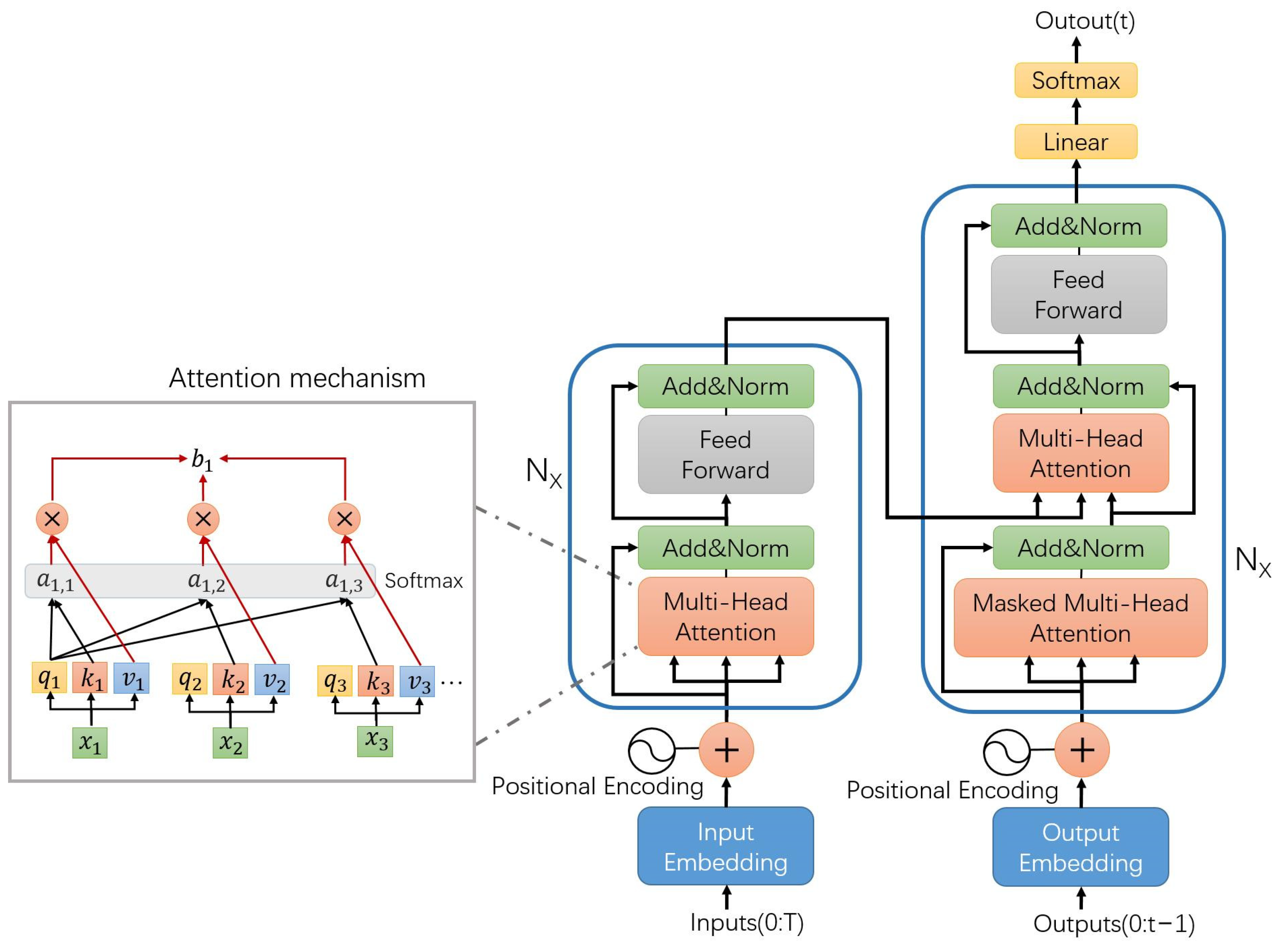
The Transformer is an advanced deep learning model originally designed for text processing, proposed by A. Vaswani et al. [37]. The core component of the model is the self-attention mechanism. In RNN, the model focuses on the input of the unit at time t and the output of the unit at time t − 1. In contrast, the Transformer, through its attention mechanism, allows the model to see the entire input sequence at any given moment. This enables the model to attend to global information within the input sequence during prediction, facilitating the capture of long-range dependencies, thereby enhancing model performance and interpretability [106,107,108]. Additionally, the Transformer model has replaced traditional RNN in various fields through its self-attention mechanism. As shown in Figure 20, the Transformer model consists of two parts, the encoder and the decoder. The encoder processes the input sequence and embeds it. It encodes the input into high-dimensional vectors using a multi-head attention mechanism to handle the input sequence and capture dependencies between elements, ultimately outputting a continuous vector that contains information from the input sequence. The decoder receives the output from the encoder and mixes it with the previous decoder outputs, passing it through the decoder, and after processing through a multi-head attention mechanism, outputs the target sequence at that moment [100]. To ensure that the model performs consistently during training and testing, Masked Multi-head attention is used in decoder training to make the decoder focus only on the outputs of the unit before time t. In the attention mechanism, the high-dimensional vectors transformed from the input are multiplied by weight matrices W Q , W K , W V and mapped into three different vector sets: query vectors Q, key vectors K, and value vectors V. The attention weights are calculated through the dot product of Q and K, normalized by a Softmax function, and then multiplied by V to obtain a vector set that incorporates different attention weights. The attention function is shown in Equation (44):
A t t e n t i o n ( Q , K , V ) = softmax ( Q K T d k ) V
where d k is the size of each key vector. Multi-head attention is used in Transformer, as shown in Equations (45) and (46). In the attention mechanism, each input sequence unit is operated with multiple sets of different weight matrices to obtain multiple sets of attention weight vector sets and then output after concatenation.
M u l t i H e a d A t t e n t i o n ( Q , K , V ) = C o n c a t ( h e a d 1 , , h e a d H )
h e a d i = A t t e n t i o n ( Q W i Q , K W i K , V W i V )
The multi-head attention mechanism allows the model to focus on multiple important input pieces of information based on different criteria, enabling the model to effectively capture various complex relationships between different elements in a sequence [109]. Moreover, compared to RNN, Transformer, by employing the multi-head self-attention mechanism, eliminates the recurrent structure, alleviating the training difficulties of recurrent neural network architectures such as LSTM and GRU, which cannot fully utilize the parallel computing capabilities of GPUs. This allows the model to better leverage GPU parallel computing and process the entire sequence simultaneously, accelerating the training speed [110].
Currently, Transformer has achieved certain research progress in estimating battery characteristics and monitoring battery status, showing superior performance compared to RNN. M. A. Hannan et al. [111] used a self-supervised Transformer model to achieve an accurate estimation of the SOC. The study utilized datasets from LG and Panasonic batteries, which included data under various temperature and driving cycle conditions. By inputting voltage, current, and temperature, the model learns the mapping relationship between input features and SOC and outputs the battery’s SOC estimation. To verify the model’s performance, the study compared the proposed model with the performance of other deep learning architectures such as LSTM, GRU, and CNN. The results show that the model outperforms these methods in terms of SOC estimation accuracy, achieving an RMSE of 0.90% and an MAE of 0.44% under constant ambient temperature conditions and an RMSE of 1.19% and an MAE of 0.7% under varying ambient temperature conditions. Ruizhi Hu et al. [112], to address computational efficiency and hardware implementation issues in battery SOC estimation, proposed a model based on RNN and Transformer using local RNN and a multi-head self-attention mechanism to capture regional and long-term dependencies in sequential data. The study used three different battery datasets: the Turnigy Graphene battery dataset, the LG HG2 dataset, and the Samsung INR21700 30T dataset, which included parameters such as instantaneous current, voltage, the temperature difference between the battery and the environment, and SOC. By inputting the current, voltage, and the temperature difference between the battery and the ambient environment, the model outputs the SOC estimation. On the Turnigy Graphene dataset, the LISA model achieved an average RMSE of 2.10%, which is quite good. By employing transfer learning methods, even with a small amount of training data, the model can achieve a low RMSE (below 5%) on the LG HG2 dataset, significantly reducing the demand for training data. The model combined with a multi-head self-attention mechanism has low computational complexity, few training parameters (only 298), and low floating-point operation times (1.18 K FLOPs), which make it possible to realize a lightweight BTMS design for real-time monitoring of battery status on the vehicle side.
Currently, in the application of battery thermal management, Transformer can handle long-sequence data and capture long-term dependencies within time series, which is crucial for predictive and diagnostic tasks in battery thermal management. In future research, it could be explored how to use Transformer for the continuous monitoring of parameters such as battery temperature and voltage to predict whether a battery might be at risk of thermal runaway. Additionally, by employing simplified Transformer structures or integrating the multi-head attention mechanism with other deep learning models, it may be possible to achieve real-time monitoring of battery operation temperature and status, quickly identifying and diagnosing abnormal battery behavior.

4.3. Kolmogorov–Arnold Network (KAN)

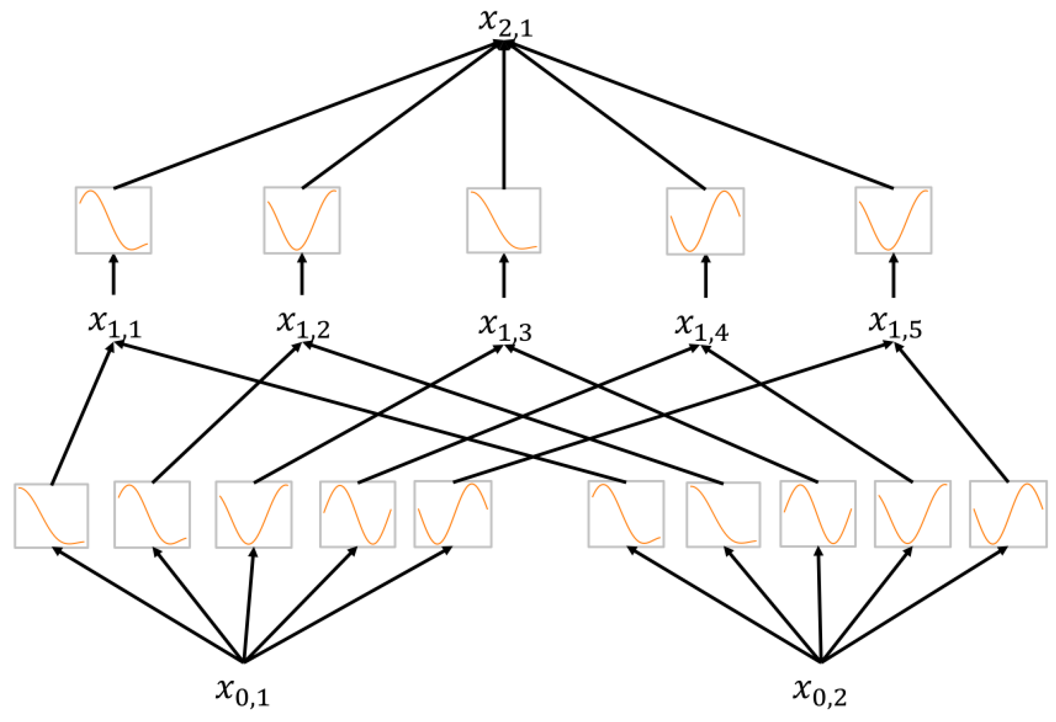
Recently, the Kolmogorov–Arnold Network (KAN) has garnered widespread attention. This algorithm, proposed by Ziming Liu et al. [35], is an improved deep learning framework inspired by the Kolmogorov–Arnold representation theorem [113,114,115], which states that any multivariate continuous function can be represented as a superposition of one-dimensional functions, as shown in Equation (47). A multivariate function f ( x 1 , , x n ) can be represented by a KAN with just two layers. In the work of Ziming Liu and colleagues, the Kolmogorov–Arnold representation was extended to neural networks of arbitrary width and depth, addressing the limitations in previous studies where network dimensions restricted their performance in fitting complex problems.
f ( x 1 , , x n ) = q = 0 2 n Φ q ( p = 1 n Ψ q , p ( x p ) )
As shown in Figure 21, unlike the traditional Multi-layer Perceptron (MLP) that uses fixed activation functions, KAN employs learnable activation functions. This allows each weight parameter in KAN to be replaced by a univariate function, which is parameterized by a B-spline curve, as shown in Equation (48). This design enables KAN to decompose complex high-dimensional functions into a series of simple one-dimensional function combinations, allowing the network to model complex functions with fewer parameters. It also provides more intuitive feedback on how the model responds to input changes, greatly enhancing the interpretability of the model. During KAN training, the target function is fitted by adjusting the basic functions of the B-spline curve, and techniques such as Sparsification and Pruning are used to simplify the network further.
φ ( x ) = i = 0 n c i B i ( x )
Research indicates that KAN outperforms MLP in terms of accuracy and interpretability. Even with a smaller scale, KAN can achieve comparable or better accuracy than a larger MLP in small-scale AI + Science tasks. In the study by Ziming Liu et al., despite the KAN model having three orders of magnitude fewer parameters than MLP, it still achieved a higher accuracy rate in the signature classification problem. Additionally, KAN is more effective than MLP in science-related tasks such as fitting physical equations and solving partial differential equations (PDEs). In the future, KAN may find applications in solving tasks such as the Navier-Stokes equations and density functional theory. This method, which combines deep learning with traditional mathematical representation, opens up new possibilities for understanding and interpreting deep learning models.
Currently, deep learning models developed for battery thermal management systems are not efficient and have relatively complex structures, requiring improvement. The proposal of KAN can be considered a method to simplify deep learning models and greatly enhance model interpretability. With its ideal performance in fitting physical equations, KAN could be used in the future to handle the coupling relationships of multiple physical fields such as heat, electricity, and chemical reactions in battery thermal management, providing a more comprehensive solution. Compared to traditional neural networks, KAN has fewer parameters, a more simplified model, and is composed of interpretable functions. By learning relevant battery data and operational characteristics, KAN could be applied in identifying potential patterns of battery thermal behavior, monitoring battery temperature, adjusting thermal management measures, and preemptively identifying the risk of thermal runaway, helping to design more efficient, safe, and interpretable thermal management systems for automotive batteries. However, compared to MLP, the different activation functions in KAN cannot utilize batch computation, resulting in KAN’s training speed typically being 10 times slower than MLP’s under the same parameter volume, which is the biggest bottleneck for KAN at present. Fortunately, in the application of deep learning-assisted thermal management systems, the final accuracy of the model is more valued than the training time, and it is believed that with the continuous emergence of subsequent optimization algorithms, this drawback will be remedied, making KAN superior to MLP in all aspects.

5. Summary

Currently, various deep learning algorithms are crucial for advancing BTMS in new energy electric vehicles, facilitating the prediction of batteries’ thermal and electrical properties as well as overall system performance. This paper delineates the foundational principles and practical applications of prevalent deep learning techniques in battery thermal management. It provides an overview of state-of-the-art models introduced in recent years. These deep learning approaches are designed to minimize computational demands while sustaining high model accuracy, with the selection of a technique contingent upon the specific research context, objectives, and data characteristics.
CNNs are particularly well-suited for the real-time monitoring of battery spatial temperatures, which is essential for thermal runaway alerts. The integration of CNNs with external sensors ensures the precise acquisition of the battery’s internal temperature and contributes to cost reduction [63]. To enhance the model’s adaptability to the features derived from battery data, augmenting the network’s depth is an effective strategy. Moreover, incorporating residual connections in deep networks effectively mitigates the degradation issue commonly encountered in such architectures. RNNs and their derivatives excel in forecasting future battery temperature trends by capturing temporal dynamics [81]. Although CNNs can deliver accurate predictions for battery time series data through convolutional operations [64,66], their requirement for multi-layer processing in lengthy sequences can escalate computational demands, potentially hindering their implementation on mobile vehicular platforms. The Transformer model leverages the attention mechanism to address the long-term dependency issues inherent in RNNs and to enhance model interpretability. Despite its higher computational complexity, the attention mechanism’s ability to perform parallel computations offers a distinct advantage over the sequential processing characteristic of RNNs. Incorporating the multi-head attention mechanism of Transformers with localized RNNs represents an innovative approach that promises optimal SOC prediction with minimal training parameters and a reduced count of floating-point operations [112]. Generative models, including GANs and DMs, are instrumental in augmenting limited battery datasets and bolstering model training [90,92]. Their integration into the development of BTMS prediction models fosters enhanced generalization and robustness. The recently introduced KAN model employs learnable activation functions diverging from the conventional fixed functions and weights, thereby streamlining the network architecture and enhancing interpretability. Although KAN has yet to be applied in battery thermal management, its exemplary performance in modeling physical equations positions it as a promising candidate for addressing the complex interplay of thermal, electrical, and chemical phenomena in battery thermal management systems.

6. Discussion and Future Prospects

Due to the rapid development of new energy vehicles, the capacity and energy density of batteries are also increasing, which increases the challenge of battery thermal management. Given the current development of deep learning algorithms, we analyze the current development bottlenecks of deep learning in BTMS applications and provide potential solutions and development directions for future research.
(1) Models with Reduced Data Dependency: Currently, diverse battery datasets are often used for training to ensure the accuracy and stability of deep learning models. Although training datasets can be constructed from publicly available laboratory data and simulation calculations, data from NEVs operating under complex and variable real-world conditions are more meaningful for the development of advanced BTMS. However, due to confidentiality policies, most NEV manufacturers do not disclose actual battery operation data [85]. This results in a limited availability of real-world NEV battery data for deep learning. In this context, models that can learn from a small batch of data effectively, capture key features, and reduce dependency on data samples represent a future development direction for BTMS applications. Additionally, using generative models to accurately expand limited datasets with a small amount of real NEV operation data is a feasible method to alleviate the current data scarcity [85,90,92]. In addition, some neural networks combined with physical information often show excellent results under a small amount of training data by learning the physical relationships between data for fitting, which is also worth exploring in future work.
(2) Simplified and Computationally Efficient Models: In order to enhance the performance of deep learning models, it is often necessary to increase the number of network layers to achieve better nonlinear fitting effects. However, on NEVs, due to the limitations of onboard processor computing power and memory, models with fewer parameters and lower computational requirements are more suitable for future deployment in vehicles. For instance, CNNs show excellent performance in handling spatial distribution data, but these networks typically have a large number of parameters [30,68], and most of them do not contribute to the actual prediction of the model, leading to parameter redundancy and increased computational complexity. Certain CNN designs, specifically those crafted for lightweight deployment [116], offer a promising approach by striking a balance between model compactness and computational efficiency, providing inspiration for further research. Employing these lightweight models in place of their more complex counterparts presents a productive strategy to mitigate parameter redundancy within current BTMS models, facilitating their effective integration into resource-constrained environments, such as those found in automotive terminals. Currently, the domain of BTMS suffers from a lack of research dedicated to lightweight network models. Developing simplified and efficient models that conserve memory space and expedite estimation processes represents an imperative direction for future research. This focus is crucial for the application of deep learning models in the thermal management of batteries within new energy vehicles, ensuring their suitability for next-generation systems. Currently, the field of BTMS is marked by a significant gap in research about lightweight network models. The development of streamlined, high-efficiency models that reduce memory footprint and expedite estimation processes is a critical research avenue for the application of deep learning in new energy vehicle BTMS. This approach is essential for optimizing model performance within the constraints of vehicular environments.
(3) Multi-physics Coupled Models: In battery thermal management, properties such as temperature are often the result of multiple factors, and temperature trends are influenced by various aspects such as internal chemical activity and internal resistance. Current predictions of battery temperature and SOC often consider factors too singularly. Models capable of multi-physics coupling and capturing the interplay between various data can significantly enhance predictive performance and more accurately reflect the actual operation of batteries.
(4) Models with Stronger Interpretability: The prevalent application of “black box” deep learning models in battery thermal management presents challenges in deciphering the model’s estimation of the current battery state and its predictions of future states based on input data. The integration of mathematically transparent technologies, such as the Transformer’s attention mechanism and KAN, will facilitate a deeper exploration of the relationships between battery parameters, heating rates, temperature, and the model’s internal mechanisms, thereby enhancing the development of BTMS. This approach will enable researchers to discern less effective parameters within the model, allowing for their simplification and creating a streamlined prediction model. Such a model, characterized by a reduced parameter set and enhanced performance, will be instrumental in the design of efficient, lightweight BTMS solutions.
(5) Models with Cross-algorithm Integration: In recent years, the deployment of deep learning within BTMS has transcended the use of singular algorithms, embracing hybrid models that integrate two or more algorithms. For instance, the models referenced in Ref. [80], Ref. [81], and Ref. [112] demonstrate that by blending various deep learning techniques and leveraging the strengths of each, a hybrid approach can significantly enhance model performance. For future BTMS designs in new energy electric vehicles, precise real-time operational assessment mandates that predictive models acquire multi-modal battery data. This necessitates the integration of diverse deep learning technologies within the model to enable the BTMS to make more precise judgments and to adjust temperature control strategies promptly.

Author Contributions

Conceptualization, S.Q.; Data management, S.Q. and Z.L.; Formal analysis, S.Q., C.Z. and Y.C.; Surveys, S.Q. and C.Z.; Methodology, S.Q., C.Z. and J.W.; Project Management, C.Z.; Resources, S.Q.; Supervision, C.Z.; Validation, S.Q. and C.Z.; Visualization, S.Q.; Writing—first draft, S.Q. Writing—proofreading and editing, C.Z., H.L. and Y.C. All authors have read and agreed to the published version of the manuscript.

Funding

This research was funded by the Department of Science and Technology of Jilin Province (grant number: 20230402077GH), China.

Data Availability Statement

Data will be made available on request.

Conflicts of Interest

The authors declare no conflicts of interest.

References

  1. Onn, C.C.; Chai, C.; Abd Rashid, A.F.; Karim, M.R.; Yusoff, S. Vehicle electrification in a developing country: Status and issue, from a well-to-wheel perspective. Transp. Res. Part D Transp. Environ. 2017, 50, 192–201. [Google Scholar] [CrossRef]
  2. Xu, B.; Lin, B.Q. Differences in regional emissions in China’s transport sector: Determinants and reduction strategies. Energy 2016, 95, 459–470. [Google Scholar] [CrossRef]
  3. Wang, G.; Guo, X.; Chen, J.; Han, P.; Su, Q.; Guo, M.; Wang, B.; Song, H. Safety Performance and Failure Criteria of Lithium-Ion Batteries under Mechanical Abuse. Energies 2023, 16, 6346. [Google Scholar] [CrossRef]
  4. Sun, S.H.; Wang, W.C. Analysis on the market evolution of new energy vehicle based on population competition model. Transp. Res. Part D Transp. Environ. 2018, 65, 36–50. [Google Scholar] [CrossRef]
  5. Ali, A.; Shakoor, R.; Raheem, A.; Muqeet, H.A.u.; Awais, Q.; Khan, A.A.; Jamil, M. Latest energy storage trends in multi-energy standalone electric vehicle charging stations: A comprehensive study. Energies 2022, 15, 4727. [Google Scholar] [CrossRef]
  6. Yuan, X.D.; Cai, Y.C. Forecasting the development trend of low emission vehicle technologies: Based on patent data. Technol. Forecast. Soc. Chang. 2021, 166, 120651. [Google Scholar] [CrossRef]
  7. He, W.; Li, Z.; Liu, T.; Liu, Z.; Guo, X.; Du, J.; Li, X.; Sun, P.; Ming, W. Research progress and application of deep learning in remaining useful life, state of health and battery thermal management of lithium batteries. J. Energy Storage 2023, 70, 107868. [Google Scholar] [CrossRef]
  8. Jaguemont, J.; Van Mierlo, J. A comprehensive review of future thermal management systems for battery-electrified vehicles. J. Energy Storage 2020, 31, 101551. [Google Scholar] [CrossRef]
  9. Liang, L.; Zhao, Y.; Diao, Y.; Ren, R.; Zhang, L.; Wang, G. Optimum cooling surface for prismatic lithium battery with metal shell based on anisotropic thermal conductivity and dimensions. J. Power Sources 2021, 506, 230182. [Google Scholar] [CrossRef]
  10. Hannan, M.A.; Hoque, M.M.; Mohamed, A.; Ayob, A. Review of energy storage systems for electric vehicle applications: Issues and challenges. Renew. Sustain. Energy Rev. 2017, 69, 771–789. [Google Scholar] [CrossRef]
  11. Wang, Q.; Jiang, B.; Li, B.; Yan, Y. A critical review of thermal management models and solutions of lithium-ion batteries for the development of pure electric vehicles. Renew. Sustain. Energy Rev. 2016, 64, 106–128. [Google Scholar] [CrossRef]
  12. Pavlovskii, A.A.; Pushnitsa, K.; Kosenko, A.; Novikov, P.; Popovich, A.A. Organic anode materials for lithium-ion batteries: Recent progress and challenges. Materials 2022, 16, 177. [Google Scholar] [CrossRef]
  13. Nguyen, T.D.; Deng, J.; Robert, B.; Chen, W.; Siegmund, T. Experimental investigation on cooling of prismatic battery cells through cell integrated features. Energy 2022, 244, 122580. [Google Scholar] [CrossRef]
  14. Tete, P.R.; Gupta, M.M.; Joshi, S.S. Developments in battery thermal management systems for electric vehicles: A technical review. J. Energy Storage 2021, 35, 102255. [Google Scholar] [CrossRef]
  15. Al Miaari, A.; Ali, H.M. Batteries temperature prediction and thermal management using machine learning: An overview. Energy Rep. 2023, 10, 2277–2305. [Google Scholar] [CrossRef]
  16. Jay, R.P.; Manish, K.R. Phase change material selection using simulation-oriented optimization to improve the thermal performance of lithium-ion battery. J. Energy Storage 2022, 49, 103974. [Google Scholar] [CrossRef]
  17. Liu, H.; Wei, Z.; He, W.; Zhao, J. Thermal issues about Li-ion batteries and recent progress in battery thermal management systems: A review. Energy Convers. Manag. 2017, 150, 304–330. [Google Scholar] [CrossRef]
  18. Jaewan, K.; Jinwoo, O.; Hoseong, L. Review on battery thermal management system for electric vehicles. Appl. Therm. Eng. 2019, 149, 192–212. [Google Scholar] [CrossRef]
  19. Muench, S.; Wild, A.; Friebe, C.; Häupler, B.; Janoschka, T.; Schubert, U.S. Polymer-Based Organic Batteries. Chem. Rev. 2016, 116, 9438–9484. [Google Scholar] [CrossRef] [PubMed]
  20. Cui, X.; Zeng, J.; Zhang, H.; Yang, J.; Qiao, J.; Li, J.; Li, W. Simplification strategy research on hard-cased Li-ion battery for thermal modeling. Int. J. Energy Res. 2020, 44, 3640–3656. [Google Scholar] [CrossRef]
  21. Jin, S.-Q.; Li, N.; Bai, F.; Chen, Y.-J.; Feng, X.-Y.; Li, H.-W.; Gong, X.-M.; Tao, W.-Q. Data-driven model reduction for fast temperature prediction in a multi-variable data center. Int. Commun. Heat Mass Transf. 2023, 142, 106645. [Google Scholar] [CrossRef]
  22. Li, A.; Weng, J.; Yuen, A.C.Y.; Wang, W.; Liu, H.; Lee, E.W.M.; Wang, J.; Kook, S.; Yeoh, G.H. Machine learning assisted advanced battery thermal management system: A state-of-the-art review. J. Energy Storage 2023, 60, 106688. [Google Scholar] [CrossRef]
  23. Sandeep Dattu, C.; Chaithanya, A.; Jeevan, J.; Satyam, P.; Michael, F.; Roydon, F. Comparison of lumped and 1D electrochemical models for prismatic 20Ah LiFePO4 battery sandwiched between minichannel cold-plates. Appl. Therm. Eng. 2021, 199, 117586. [Google Scholar] [CrossRef]
  24. Fang, P.; Zhang, A.; Wang, D.; Sui, X.; Yin, L. Lumped model of Li-ion battery considering hysteresis effect. J. Energy Storage 2024, 86, 111185. [Google Scholar] [CrossRef]
  25. Lenz, C.; Hennig, J.; Tegethoff, W.; Schweiger, H.G.; Koehler, J. Analysis of the Interaction and Variability of Thermal Decomposition Reactions of a Li-ion Battery Cell. J. Electrochem. Soc. 2023, 170, 060523. [Google Scholar] [CrossRef]
  26. Zhang, C.; Zhou, L.; Xiao, Q.; Bai, X.; Wu, B.; Wu, N.; Zhao, Y.; Wang, J.; Feng, L. End-to-end fusion of hyperspectral and chlorophyll fluorescence imaging to identify rice stresses. Plant Phenomics 2022, 2022, 9851096. [Google Scholar] [CrossRef]
  27. Talaei Khoei, T.; Ould Slimane, H.; Kaabouch, N. Deep learning: Systematic review, models, challenges, and research directions. Neural Comput. Appl. 2023, 35, 23103–23124. [Google Scholar] [CrossRef]
  28. Bao, S.D.; Wang, T.T.; Zhou, L.L.; Dai, G.L.; Sun, G.; Shen, J. Two-Layer Matrix Factorization and Multi-Layer Perceptron for Online Service Recommendation. Appl. Sci. 2022, 12, 7369. [Google Scholar] [CrossRef]
  29. Zhu, F.; Chen, J.; Ren, D.; Han, Y. Transient temperature fields of the tank vehicle with various parameters using deep learning method. Appl. Therm. Eng. 2023, 230, 120697. [Google Scholar] [CrossRef]
  30. Xu, Y.; Zhao, J.P.; Chen, J.Q.; Zhang, H.C.; Feng, Z.X.; Yuan, J.L. Performance analyses on the air cooling battery thermal management based on artificial neural networks. Appl. Therm. Eng. 2024, 252, 123567. [Google Scholar] [CrossRef]
  31. O’shea, K.; Nash, R. An introduction to convolutional neural networks. arXiv 2015, arXiv:1511.08458. [Google Scholar]
  32. Hochreiter, S.; Schmidhuber, J. Long short-term memory. Neural Comput. 1997, 9, 1735–1780. [Google Scholar] [CrossRef] [PubMed]
  33. Chung, J.; Gulcehre, C.; Cho, K.; Bengio, Y. Empirical evaluation of gated recurrent neural networks on sequence modeling. arXiv 2014, arXiv:1412.3555. [Google Scholar]
  34. Goodfellow, I.J.; Pouget-Abadie, J.; Mirza, M.; Xu, B.; Warde-Farley, D.; Ozair, S.; Courville, A.; Bengio, Y. Generative Adversarial Nets. In Proceedings of the Advances in Neural Information Processing Systems 27 (Nips 2014), Montreal, QC, Canada, 8–13 December 2014; pp. 2672–2680. [Google Scholar]
  35. Liu, Z.; Wang, Y.; Vaidya, S.; Ruehle, F.; Halverson, J.; Soljačić, M.; Hou, T.Y.; Tegmark, M. Kan: Kolmogorov-Arnold networks. arXiv 2024, arXiv:2404.19756. [Google Scholar]
  36. Sohl-Dickstein, J.; Weiss, E.; Maheswaranathan, N.; Ganguli, S. Deep unsupervised learning using nonequilibrium thermodynamics. In Proceedings of the 32nd International Conference on Machine Learning, Lille, France, 6–11 July 2015; pp. 2256–2265. [Google Scholar]
  37. Vaswani, A.; Shazeer, N.; Parmar, N.; Uszkoreit, J.; Jones, L.; Gomez, A.N.; Kaiser, L.; Polosukhin, I. Attention Is All You Need. In Proceedings of the Advances in Neural Information Processing Systems 30 (Nips 2017), Long Beach, CA, USA, 4–9 December 2017. [Google Scholar]
  38. Angelov, P.P.; Soares, E.A.; Jiang, R.; Arnold, N.I.; Atkinson, P.M. Explainable artificial intelligence: An analytical review. WIREs Data Min. Knowl. Discov. 2021, 11, e1424. [Google Scholar] [CrossRef]
  39. Hossein, M.-R.; Rata, R.; Sompop, B.; Joachim, K.; Falk, S. Deep learning: A primer for dentists and dental researchers. J. Dent. 2023, 130, 104430. [Google Scholar] [CrossRef]
  40. Guo, C.; Liu, L.; Sun, H.; Wang, N.; Zhang, K.; Zhang, Y.; Zhu, J.; Li, A.; Bai, Z.; Liu, X. Predicting Fv/Fm and evaluating cotton drought tolerance using hyperspectral and 1D-CNN. Front. Plant Sci. 2022, 13, 1007150. [Google Scholar] [CrossRef] [PubMed]
  41. Ruder, S. An overview of gradient descent optimization algorithms. arXiv 2016, arXiv:1609.04747. [Google Scholar]
  42. Robbins, H.; Monro, S. A stochastic approximation method. Ann. Math. Stat. 1951, 400–407. [Google Scholar] [CrossRef]
  43. LeCun, Y.; Bengio, Y.; Hinton, G. Deep learning. Nature 2015, 521, 436–444. [Google Scholar] [CrossRef]
  44. Rumelhart, D.E.; Hinton, G.E.; Williams, R.J. Learning representations by back-propagating errors. Nature 1986, 323, 533–536. [Google Scholar] [CrossRef]
  45. Liu, Y.; Gao, Y.; Yin, W. An improved analysis of stochastic gradient descent with momentum. In Proceedings of the Advances in Neural Information Processing Systems, Virtual, 6–12 December 2020; pp. 18261–18271. [Google Scholar]
  46. Sun, S.; Cao, Z.; Zhu, H.; Zhao, J. A survey of optimization methods from a machine learning perspective. IEEE Trans. Cybern. 2019, 50, 3668–3681. [Google Scholar] [CrossRef]
  47. Goodfellow, I.; Bengio, Y.; Courville, A. Deep Learning; MIT Press: Cambridge, MA, USA, 2016. [Google Scholar]
  48. Persson Hodén, K.; Hu, X.; Martinez, G.; Dixelius, C. smartpare: An r package for efficient identification of true mRNA cleavage sites. Int. J. Mol. Sci. 2021, 22, 4267. [Google Scholar] [CrossRef]
  49. Duchi, J.; Hazan, E.; Singer, Y. Adaptive Subgradient Methods for Online Learning and Stochastic Optimization. J. Mach. Learn. Res. 2011, 12, 2121–2159. [Google Scholar]
  50. Bassiouni, M.M.; Chakrabortty, R.K.; Hussain, O.K.; Rahman, H.F. Advanced deep learning approaches to predict supply chain risks under COVID-19 restrictions. Expert Syst. Appl. 2023, 211, 118604. [Google Scholar] [CrossRef] [PubMed]
  51. Reyad, M.; Sarhan, A.M.; Arafa, M. A modified Adam algorithm for deep neural network optimization. Neural Comput. Appl. 2023, 35, 17095–17112. [Google Scholar] [CrossRef]
  52. Kingma, D.P.; Ba, J. Adam: A method for stochastic optimization. arXiv 2014, arXiv:1412.6980. [Google Scholar]
  53. Micikevicius, P.; Narang, S.; Alben, J.; Diamos, G.; Elsen, E.; Garcia, D.; Ginsburg, B.; Houston, M.; Kuchaiev, O.; Venkatesh, G. Mixed precision training. arXiv 2017, arXiv:1710.03740. [Google Scholar]
  54. Li, H.; Wang, Y.; Hong, Y.; Li, F.; Ji, X. Layered mixed-precision training: A new training method for large-scale AI models. J. King Saud Univ. Comput. Inf. Sci. 2023, 35, 101656. [Google Scholar] [CrossRef]
  55. Paszke, A.; Gross, S.; Massa, F.; Lerer, A.; Bradbury, J.; Chanan, G.; Killeen, T.; Lin, Z.M.; Gimelshein, N.; Antiga, L.; et al. PyTorch: An Imperative Style, High-Performance Deep Learning Library. In Proceedings of the Advances in Neural Information Processing Systems 32 (Nips 2019), Vancouver, BC, Canada, 8–14 December 2019. [Google Scholar]
  56. Abadi, M.; Barham, P.; Chen, J.; Chen, Z.; Davis, A.; Dean, J.; Devin, M.; Ghemawat, S.; Irving, G.; Isard, M. {TensorFlow}: A system for {Large-Scale} machine learning. In Proceedings of the 12th USENIX Symposium on Operating Systems Design and Implementation (OSDI 16), Berkeley, CA, USA, 2–4 November 2016; pp. 265–283. [Google Scholar]
  57. Adedigba, A.P.; Adeshina, S.A.; Aibinu, A.M. Performance Evaluation of Deep Learning Models on Mammogram Classification Using Small Dataset. Bioengineering 2022, 9, 161. [Google Scholar] [CrossRef]
  58. Wang, S.F.; Wang, H.W.; Perdikaris, P. Learning the solution operator of parametric partial differential equations with physics-informed DeepONets. Sci. Adv. 2021, 7, eabi8605. [Google Scholar] [CrossRef] [PubMed]
  59. Gu, J.X.; Wang, Z.H.; Kuen, J.; Ma, L.Y.; Shahroudy, A.; Shuai, B.; Liu, T.; Wang, X.X.; Wang, G.; Cai, J.F.; et al. Recent advances in convolutional neural networks. Pattern Recognit. 2018, 77, 354–377. [Google Scholar] [CrossRef]
  60. Long, H.X.; Liao, B.; Xu, X.Y.; Yang, J.L. A Hybrid Deep Learning Model for Predicting Protein Hydroxylation Sites. Int. J. Mol. Sci. 2018, 19, 2817. [Google Scholar] [CrossRef] [PubMed]
  61. Liu, F.F.; Zhou, F.L.; Ma, L. An Automatic Detection Framework for Electrical Anomalies in Electrified Rail Transit System. IEEE Trans. Instrum. Meas. 2023, 72, 3510313. [Google Scholar] [CrossRef]
  62. Mahmoudi, M.A.; Chetouani, A.; Boufera, F.; Tabia, H. Learnable pooling weights for facial expression recognition. Pattern Recognit. Lett. 2020, 138, 644–650. [Google Scholar] [CrossRef]
  63. Wang, M.Y.; Hu, W.F.; Jiang, Y.F.; Su, F.; Fang, Z. Internal temperature prediction of ternary polymer lithium-ion battery pack based on CNN and virtual thermal sensor technology. Int. J. Energy Res. 2021, 45, 13681–13691. [Google Scholar] [CrossRef]
  64. Ma, H.L.; Bao, X.Y.; Lopes, A.; Chen, L.P.; Liu, G.Q.; Zhu, M. State-of-Charge Estimation of Lithium-Ion Battery Based on Convolutional Neural Network Combined with Unscented Kalman Filter. Batteries 2024, 10, 198. [Google Scholar] [CrossRef]
  65. Sherkatghanad, Z.; Ghazanfari, A.; Makarenkov, V. A self-attention-based CNN-Bi-LSTM model for accurate state-of-charge estimation of lithium-ion batteries. J. Energy Storage 2024, 88, 111524. [Google Scholar] [CrossRef]
  66. Yalçın, S.; Panchal, S.; Herdem, M.S. A CNN-ABC model for estimation and optimization of heat generation rate and voltage distributions of lithium-ion batteries for electric vehicles. Int. J. Heat Mass Transf. 2022, 199, 123486. [Google Scholar] [CrossRef]
  67. He, K.; Zhang, X.; Ren, S.; Sun, J. Deep residual learning for image recognition. In Proceedings of the IEEE Conference on Computer Vision and Pattern Recognition, Las Vegas, NV, USA, 27–30 June 2016; pp. 770–778. [Google Scholar]
  68. Cao, X.; Du, J.; Qu, C.; Wang, J.; Tu, R. An early diagnosis method for overcharging thermal runaway of energy storage lithium batteries. J. Energy Storage 2024, 75, 109661. [Google Scholar] [CrossRef]
  69. Wang, Z.G.; Oates, T. Imaging Time-Series to Improve Classification and Imputation. In Proceedings of the Twenty-Fourth International Joint Conference on Artificial Intelligence (IJCAI), Buenos Aires, Argentina, 25–31 July 2015; pp. 3939–3945. [Google Scholar]
  70. Medsker, L.R.; Jain, L. Recurrent neural networks. Des. Appl. 2001, 5, 2. [Google Scholar]
  71. Berman, D.S.; Buczak, A.L.; Chavis, J.S.; Corbett, C.L. A Survey of Deep Learning Methods for Cyber Security. Information 2019, 10, 122. [Google Scholar] [CrossRef]
  72. Zaremba, W.; Sutskever, I.; Vinyals, O. Recurrent neural network regularization. arXiv 2014, arXiv:1409.2329. [Google Scholar]
  73. Zhang, Y.; Li, Y.F. Prognostics and health management of Lithium-ion battery using deep learning methods: A review. Renew. Sustain. Energy Rev. 2022, 161, 112282. [Google Scholar] [CrossRef]
  74. Zhang, Q.; Wang, R.Q.; Qi, Y.; Wen, F. A watershed water quality prediction model based on attention mechanism and Bi-LSTM. Environ. Sci. Pollut. Res. 2022, 29, 75664–75680. [Google Scholar] [CrossRef] [PubMed]
  75. Lee, W.; Lim, Y.-H.; Ha, E.; Kim, Y.; Lee, W.K. Forecasting of non-accidental, cardiovascular, and respiratory mortality with environmental exposures adopting machine learning approaches. Environ. Sci. Pollut. Res. 2022, 29, 88318–88329. [Google Scholar] [CrossRef] [PubMed]
  76. Yan, R.G.; Jiang, X.; Wang, W.R.; Dang, D.P.; Su, Y.J. Materials information extraction via automatically generated corpus. Sci. Data 2022, 9, 401. [Google Scholar] [CrossRef]
  77. Tao, S.Y.; Jiang, B.; Wei, X.Z.; Dai, H.F. A Systematic and Comparative Study of Distinct Recurrent Neural Networks for Lithium-Ion Battery State-of-Charge Estimation in Electric Vehicles. Energies 2023, 16, 2008. [Google Scholar] [CrossRef]
  78. Achanta, S.; Gangashetty, S.V. Deep Elman recurrent neural networks for statistical parametric speech synthesis. Speech Commun. 2017, 93, 31–42. [Google Scholar] [CrossRef]
  79. Dey, R.; Salem, F.M. Gate-variants of gated recurrent unit (GRU) neural networks. In Proceedings of the 2017 IEEE 60th International Midwest Symposium on Circuits and Systems (MWSCAS), Boston, MA, USA, 6–9 August 2017; pp. 1597–1600. [Google Scholar]
  80. Cui, Z.H.; Kang, L.; Li, L.W.; Wang, L.C.; Wang, K. A hybrid neural network model with improved input for state of charge estimation of lithium-ion battery at low temperatures. Renew. Energy 2022, 198, 1328–1340. [Google Scholar] [CrossRef]
  81. Li, M.R.; Dong, C.Y.; Xiong, B.Y.; Mu, Y.F.; Yu, X.D.; Xiao, Q.; Jia, H.J. STTEWS: A sequential-transformer thermal early warning system for lithium-ion battery safety. Appl. Energy 2022, 328, 119965. [Google Scholar] [CrossRef]
  82. Bamati, S.; Chaoui, H.; Gualous, H. Virtual Temperature Sensor in Battery Thermal Management System Using LSTM-DNN. In Proceedings of the 2023 IEEE Vehicle Power and Propulsion Conference (VPPC), Milan, Italy, 24–27 October 2023; pp. 1–6. [Google Scholar]
  83. Yao, Q.; Lu, D.D.-C.; Lei, G. A surface temperature estimation method for lithium-ion battery using enhanced GRU-RNN. IEEE Trans. Transp. Electrif. 2022, 9, 1103–1112. [Google Scholar] [CrossRef]
  84. Li, D.; Liu, P.; Zhang, Z.S.; Zhang, L.; Deng, J.J.; Wang, Z.P.; Dorrell, D.G.; Li, W.H.; Sauer, D.U. Battery Thermal Runaway Fault Prognosis in Electric Vehicles Based on Abnormal Heat Generation and Deep Learning Algorithms. IEEE Trans. Power Electron. 2022, 37, 8513–8525. [Google Scholar] [CrossRef]
  85. Naaz, F.; Herle, A.; Channegowda, J.; Raj, A.; Lakshminarayanan, M. A generative adversarial network-based synthetic data augmentation technique for battery condition evaluation. Int. J. Energy Res. 2021, 45, 19120–19135. [Google Scholar] [CrossRef]
  86. Zhou, T.; Li, Q.; Lu, H.; Cheng, Q.; Zhang, X. GAN review: Models and medical image fusion applications. Inf. Fusion 2023, 91, 134–148. [Google Scholar] [CrossRef]
  87. Su, Y.H.; Meng, L.; Kong, X.J.; Xu, T.L.; Lan, X.S.; Li, Y.F. Generative Adversarial Networks for Gearbox of Wind Turbine with Unbalanced Data Sets in Fault Diagnosis. IEEE Sens. J. 2022, 22, 13285–13298. [Google Scholar] [CrossRef]
  88. Que, Y.; Dai, Y.; Ji, X.; Leung, A.K.; Chen, Z.; Jiang, Z.L.; Tang, Y.C. Automatic classification of asphalt pavement cracks using a novel integrated generative adversarial networks and improved VGG model. Eng. Struct. 2023, 277, 115406. [Google Scholar] [CrossRef]
  89. Wang, K.F.; Gou, C.; Duan, Y.J.; Lin, Y.L.; Zheng, X.H.; Wang, F.Y. Generative Adversarial Networks: Introduction and Outlook. IEEE/CAA J. Autom. Sin. 2017, 4, 588–598. [Google Scholar] [CrossRef]
  90. Qiu, X.H.; Wang, S.F.; Chen, K. A conditional generative adversarial network-based synthetic data augmentation technique for battery state-of-charge estimation. Appl. Soft Comput. 2023, 142, 110281. [Google Scholar] [CrossRef]
  91. Li, H.; Chen, G.H.; Yang, Y.Z.; Shu, B.Y.; Liu, Z.J.; Peng, J. Adversarial learning for robust battery thermal runaway prognostic of electric vehicles. J. Energy Storage 2024, 82, 110381. [Google Scholar] [CrossRef]
  92. Hu, F.S.; Dong, C.Y.; Tian, L.Y.; Mu, Y.F.; Yu, X.D.; Jia, H.J. CWGAN-GP with residual network model for lithium-ion battery thermal image data expansion with quantitative metrics. Energy Ai 2024, 16, 100321. [Google Scholar] [CrossRef]
  93. Rubner, Y.; Tomasi, C.; Guibas, L.J. The Earth Mover’s Distance as a metric for image retrieval. Int. J. Comput. Vis. 2000, 40, 99–121. [Google Scholar] [CrossRef]
  94. Chakraborty, T.; Reddy, K.S.U.; Naik, S.M.; Panja, M.; Manvitha, B. Ten years of generative adversarial nets (GANs): A survey of the state-of-the-art. Mach. Learn. Sci. Technol. 2024, 5, 011001. [Google Scholar] [CrossRef]
  95. Yang, L.; Zhang, Z.; Song, Y.; Hong, S.; Xu, R.; Zhao, Y.; Zhang, W.; Cui, B.; Yang, M.-H. Diffusion models: A comprehensive survey of methods and applications. ACM Comput. Surv. 2023, 56, 1–39. [Google Scholar] [CrossRef]
  96. Ho, J.; Jain, A.; Abbeel, P. Denoising diffusion probabilistic models. In Proceedings of the Advances in Neural Information Processing Systems, Virtual, 6–12 December 2020; pp. 6840–6851. [Google Scholar]
  97. Ramesh, A.; Dhariwal, P.; Nichol, A.; Chu, C.; Chen, M. Hierarchical text-conditional image generation with clip latents. arXiv 2022, arXiv:2204.06125. [Google Scholar]
  98. Rombach, R.; Blattmann, A.; Lorenz, D.; Esser, P.; Ommer, B. High-resolution image synthesis with latent diffusion models. In Proceedings of the IEEE/CVF Conference on Computer Vision and Pattern Recognition, New Orleans, LA, USA, 18–24 June 2022; pp. 10684–10695. [Google Scholar]
  99. Saharia, C.; Chan, W.; Saxena, S.; Li, L.; Whang, J.; Denton, E.L.; Ghasemipour, K.; Gontijo Lopes, R.; Karagol Ayan, B.; Salimans, T. Photorealistic text-to-image diffusion models with deep language understanding. In Proceedings of the Advances in Neural Information Processing Systems, New Orleans, LA, USA, 28 November–9 December 2022; pp. 36479–36494. [Google Scholar]
  100. Bandi, A.; Adapa, P.V.S.R.; Kuchi, Y.E.V.P.K. The Power of Generative AI: A Review of Requirements, Models, Input-Output Formats, Evaluation Metrics, and Challenges. Future Internet 2023, 15, 260. [Google Scholar] [CrossRef]
  101. Cao, H.Q.; Tan, C.; Gao, Z.Y.; Xu, Y.L.; Chen, G.Y.; Heng, P.A.; Li, S.Z. A Survey on Generative Diffusion Models. IEEE Trans. Knowl. Data Eng. 2024, 36, 2814–2830. [Google Scholar] [CrossRef]
  102. Casolaro, A.; Capone, V.; Iannuzzo, G.; Camastra, F. Deep Learning for Time Series Forecasting: Advances and Open Problems. Information 2023, 14, 598. [Google Scholar] [CrossRef]
  103. Croitoru, F.A.; Hondru, V.; Ionescu, R.T.; Shah, M. Diffusion Models in Vision: A Survey. IEEE Trans. Pattern Anal. Mach. Intell. 2023, 45, 10850–10869. [Google Scholar] [CrossRef]
  104. Luo, C.; Zhang, Z.; Zhu, S.; Li, Y. State-of-Health Prediction of Lithium-Ion Batteries Based on Diffusion Model with Transfer Learning. Energies 2023, 16, 3815. [Google Scholar] [CrossRef]
  105. Huang, T.; Gao, Y.; Li, Z.; Hu, Y.; Xuan, F. A hybrid deep learning framework based on diffusion model and deep residual neural network for defect detection in composite plates. Appl. Sci. 2023, 13, 5843. [Google Scholar] [CrossRef]
  106. Liu, N.; Yuan, Z.M.; Tang, Q.F. Improving Alzheimer’s Disease Detection for Speech Based on Feature Purification Network. Front. Public Health 2022, 9, 835960. [Google Scholar] [CrossRef] [PubMed]
  107. Ding, H.; Li, F.J.; Chen, X.; Ma, J.; Nie, S.P.; Ye, R.; Yuan, C.J. ContransGAN: Convolutional Neural Network Coupling Global Swin-Transformer Network for High-Resolution Quantitative Phase Imaging with Unpaired Data. Cells 2022, 11, 2394. [Google Scholar] [CrossRef] [PubMed]
  108. Chang, X.; Feng, Z.; Wu, J.; Sun, H.; Wang, G.; Bao, X. Understanding and predicting the short-term passenger flow of station-free shared bikes: A spatiotemporal deep learning approach. IEEE Intell. Transp. Syst. Mag. 2021, 14, 73–85. [Google Scholar] [CrossRef]
  109. Sajun, A.R.; Zualkernan, I.; Sankalpa, D. A Historical Survey of Advances in Transformer Architectures. Appl. Sci. 2024, 14, 4316. [Google Scholar] [CrossRef]
  110. Abibullaev, B.; Keutayeva, A.; Zollanvari, A. Deep Learning in EEG-Based BCIs: A Comprehensive Review of Transformer Models, Advantages, Challenges, and Applications. IEEE Access 2023, 11, 127271–127301. [Google Scholar] [CrossRef]
  111. Hannan, M.A.; How, D.N.T.; Lipu, M.S.H.; Mansor, M.; Ker, P.J.; Dong, Z.Y.; Sahari, K.S.M.; Tiong, S.K.; Muttaqi, K.M.; Mahlia, T.M.I.; et al. Deep learning approach towards accurate state of charge estimation for lithium-ion batteries using self-supervised transformer model. Sci. Rep. 2021, 11, 19541. [Google Scholar] [CrossRef]
  112. Hun, R.; Zhang, S.; Singh, G.; Qian, J.; Chen, Y.; Chiang, P.Y. LISA: A transferable light-weight multi-head self-attention neural network model for lithium-ion batteries state-of-charge estimation. In Proceedings of the 2021 3rd International Conference on Smart Power & Internet Energy Systems (SPIES), Shanghai, China, 25–28 September 2021; pp. 464–469. [Google Scholar]
  113. Kolmogorov, A.N. On the Representation of Continuous Functions of Several Variables by Superpositions of Continuous Functions of a Smaller Number of Variables; American Mathematical Society: Providence, RI, USA, 1961. [Google Scholar]
  114. Kolmogorov, A.N. On the representation of continuous functions of many variables by superposition of continuous functions of one variable and addition. Proc. Dokl. Akad. Nauk. 1957, 114, 953–956. [Google Scholar]
  115. Braun, J.; Griebel, M. On a Constructive Proof of Kolmogorov’s Superposition Theorem. Constr. Approx. 2009, 30, 653–675. [Google Scholar] [CrossRef]
  116. Yuan, L.; Chen, Y.; Tang, H.; Liu, Z.; Wu, W. DGNet: An adaptive lightweight defect detection model for new energy vehicle battery current collector. IEEE Sens. J. 2023, 23, 29815–29830. [Google Scholar] [CrossRef]
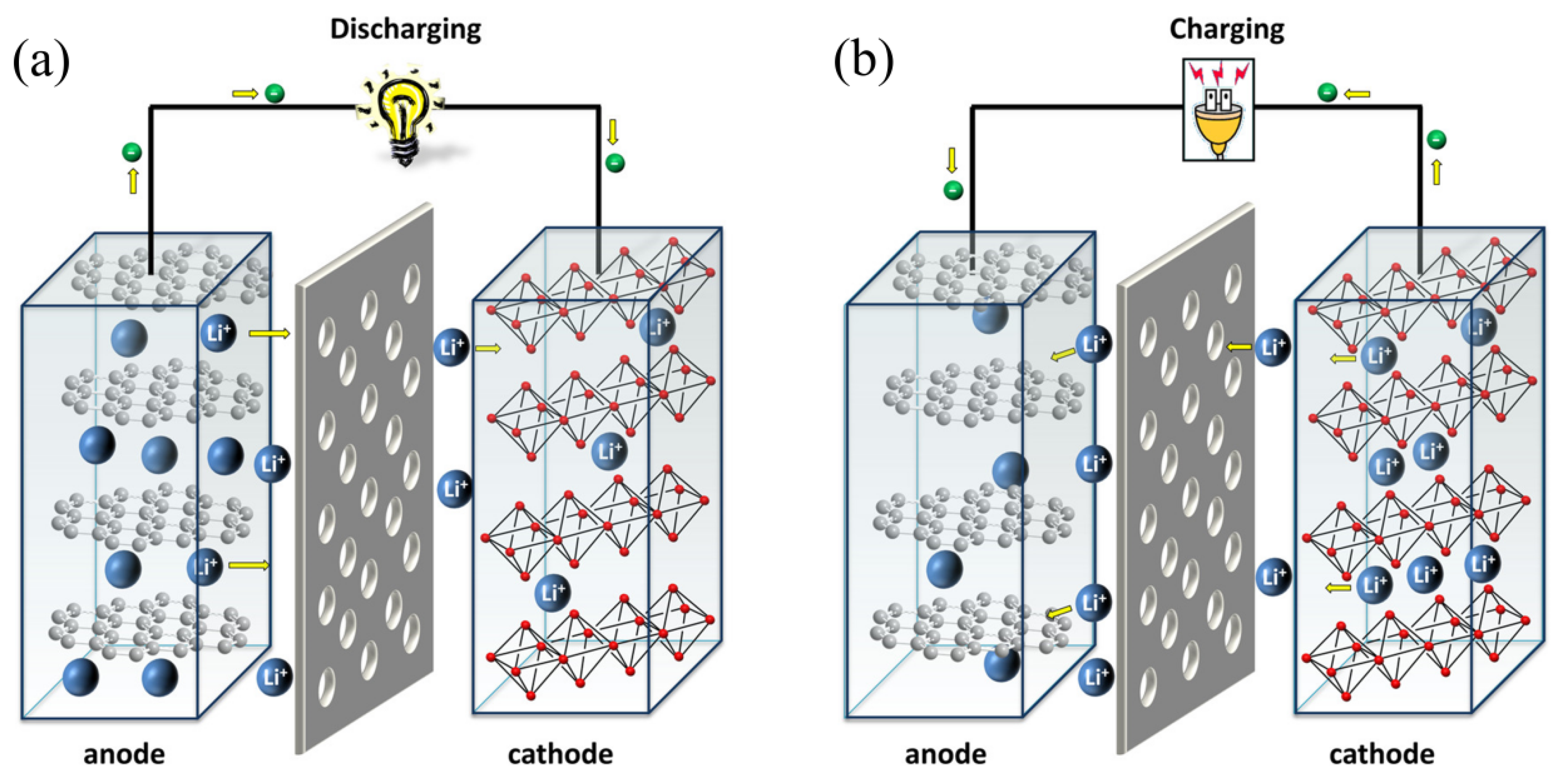
Figure 1. Schematic diagram of (a) discharging and (b) charging process of lithium-ion battery (Reprinted with permission from Ref. [19], Copyright 2016, American Chemical Society).
Energies 17 04132 g001
Figure 2. Schematic of the principles of (a) deep learning framework and (b) neurons.
Energies 17 04132 g002
Figure 3. Effects of larger and smaller learning rates on neural network parameter optimization.
Energies 17 04132 g003
Figure 4. Comparison of Gradient Descent with Momentum and Gradient Descent under (a) local optimal point gradient and (b) high curvature gradient.
Energies 17 04132 g004
Figure 5. Flowchart of the principle of mixed-precision training.
Energies 17 04132 g005
Figure 6. Schematic of (a) convolutional neural network architecture, (b) convolution operation, (c) pooling operation.
Energies 17 04132 g006
Figure 7. Overall flowchart of CNN-UKF (Figure obtained from [64]).
Energies 17 04132 g007
Figure 8. Plots of measured voltage, current, and ambient temperature for training (ac) and test (df) datasets at room temperature 25 °C. (g) Structure diagram of the CNN-Bi-LSTM-AM model (Figure obtained from [65]).
Energies 17 04132 g008
Figure 9. The proposed CNN architecture for HGR and voltage estimation (Figure obtained from [66]).
Energies 17 04132 g009
Figure 10. Schematic representations of (a) the residual neural network architecture, (b) the BTMS structure, and (c) the ResNet-50 architecture in the study (Figure obtained from [30]).
Energies 17 04132 g010
Figure 11. Model structure (Figure obtained from [68]).
Energies 17 04132 g011
Figure 12. The structures of (a) RNN, (b) LSTM, and (c) GRU.
Energies 17 04132 g012
Figure 13. The architecture of (a) 1D convolutional neural network with (b) BWGRU neural network (Figure obtained from [80]).
Energies 17 04132 g013
Figure 14. Schematic of model architecture (Figure obtained from [77]).
Energies 17 04132 g014
Figure 15. Schematic of GAN architecture (Figure obtained from [86]).
Energies 17 04132 g015
Figure 16. The proposed detection method (Figure obtained from [91]).
Energies 17 04132 g016
Figure 17. Structure of CWGAN-GP with ResNet (Figure obtained from [92]).
Energies 17 04132 g017
Figure 18. Typical structure of diffusion model.
Energies 17 04132 g018
Figure 19. The flowchart of proposed approach (Figure obtained from [104]).
Energies 17 04132 g019
Figure 20. Structure of Transformer.
Energies 17 04132 g020
Figure 21. Structure of Kolmogorov–Arnold Networks.
Energies 17 04132 g021
Table 1. Comparison of CNN and LR prediction effects [63].
ModelMSEMAEMAXER2
LR0.16410.34410.33150.9823
CNN0.0470.16570.46890.9949
Table 2. Comparison of SOC estimation results at room temperature (25 °C) with three lower ambient temperatures (10 °C, 0 °C, −10 °C) [65].
Temperature10 °C0 °C−10 °C25 °C
RMSE (%)MAE (%)RMSE (%)MAE (%)RMSE (%)MAE (%)RMSE (%)MAE (%)
LSTM1.330.791.430.871.641.071.090.78
LSTM-AM1.290.761.270.81.591.011.040.77
Bi-LSTM1.310.771.250.831.611.031.080.8
Bi-LSTM-AM1.280.771.230.781.570.931.050.76
S-LSTM1.270.761.160.751.40.861.060.78
S-LSTM-AM1.260.721.110.731.350.851.050.77
S-Bi-LSTM1.260.751.10.731.290.811.050.78
S-Bi-LSTM-AM1.250.731.080.711.280.771.050.78
CNN-LSTM1.230.770.980.631.270.80.990.67
CNN-LSTM-AM1.210.710.980.651.260.770.950.66
CNN-Bi-LSTM1.230.760.990.621.250.7810.72
CNN-Bi-LSTM-AM1.20.670.970.611.190.720.920.66
Table 3. MAE and RMSE of the estimated results of the proposed network under different temperature and different cycle conditions [80].
Temperature0 °C−10 °C−20 °C
RMSE (%)MAE (%)RMSE (%)MAE (%)RMSE (%)MAE (%)
UDDS0.008580.006590.01030.00750.01370.0104
US060.01040.008770.01450.009870.01710.0127
HWFET0.008130.005510.01440.00990.01330.00998
LA920.008570.006870.01290.009020.01590.0126
Table 4. Deep learning for battery thermal management.
Authors, YearMethodsApplicationsTraining DataPerformanceShortcomings
Mengyi Wang et al. [63], 2021CNN + VTSPredict the internal temperature of the battery.Heat map of battery external temperature versus internal temperatureThe accuracy of temperature prediction has obvious advantages over (linear regression) LR.The robustness of the model remains to be verified.
Hongli Ma et al. [64], 2024CNN + UKFPredict SOC.Voltage, current and temperature, SOCThe proposed method outperforms other data-driven SOC estimation methods in terms of accuracy and robustness.The model is sensitive to the filtering parameters, and the robustness of the model still has room for improvement.
Zeinab Sherkatghanad et al. [65], 2024CNN-Bi-LSTM-AMPredict SOC over a wide range of temperatures.SOC, current, voltage, temperature, average current, and average voltageThe model shows high estimation accuracy and prediction effect under different temperature conditions and has strong generalization ability.Electrochemical information can be incorporated to expand the features, and the accuracy of the model still has room for improvement.
S Yalçın et al. [66], 2022CNN + ABCPredict the battery HGR and voltage distribution.Current, temperature, HGR, and voltageThe RMSE of HGR estimation is 1.38%, and the R2 is 99.72%. The RMSE of voltage estimation is 3.55%, and the R2 is 99.82%.Validation for the prediction of battery life or other critical battery parameters is still lacking.
Yuan Xu et al. [30], 2024ResNetPredict BTMS performance (maximum temperature and maximum temperature difference).Cell spacing (d), main channel inclination (θ) and inlet velocity (v), Tmax, ΔTmaxThe maximum temperature error of the model is 0.08%, and the maximum temperature difference error is 2.64%.-
Xin Cao et al. [68], 2024ResNet + GASFEarly diagnosis of electrothermal runaway.2D thermodynamic image containing surface temperature time series informationA diagnostic accuracy of 97.7% is achieved before the battery surface temperature reaches 50 °C.-
Zhenhua Cui et al. [80], 2022GRU + CNNSOC estimation in low temperature environment.Voltage, current and temperature, SOCMAE and RMSE are less than 0.0127 and 0.0171, respectively.-
Siyi Tao et al. [77], 2023RNNCompare the performance of different RNN models in SOC estimation.Current, voltage, and SOCThe BLSTM model performs best under NEDC, UDDS. and WLTP conditions with MAE values of 1.05%, 7.81%. and 1.81%, respectively.-
Marui Li et al. [81], 2022LSTM + CNNEstimate battery temperature trend.Surface temperature, ambient temperature, heating rate, and SOCThe model can use 20 s of time series data to predict the surface temperature change of lithium-ion energy system in the next 60 s, and the maximum MSE reduction of the model is 0.01 compared with TCN. Compared to LSTM, the reduction can be up to 0.02.-
Safieh Bamati et al. [82], 2023LSTM + DNNEstimate the surface temperature of the battery.Voltage and current time series and their average valuesThe proposed method can accurately estimate the surface temperature in the whole aging cycle of the battery, the prediction error range is only 0.25–2.45 °C, and it shows higher prediction accuracy in the later cycle of the battery.-
Qi Yao et al. [83], 2022GRUEstimate the surface temperature of the Li-ion battery.Time series of voltage, current, SOC, and ambient temperatureIt shows good performance and generalization ability under different ambient temperature conditions and different driving cycles. The MAE is less than 0.2 °C under the fixed ambient temperature condition and less than 0.42 °C under the varying ambient temperature condition.At low temperature (−10 °C), the estimation error is higher. Under low temperature and varying temperature conditions, the estimation accuracy of the model needs to be further improved.
Da Li et al. [84], 2022LSTM + CNNPredict battery thermal runaway, temperature.Battery temperature, battery voltage, battery current, ambient temperature, etcThe battery temperature within the next 8 min can be accurately predicted with an average relative error of 0.28%.The model has high complexity and depends heavily on the quality and diversity of the training data.
Falak Naaz et al. [85], 2021GANBroaden the dataset and enhance the SOC estimation.Voltage, current, temperature, and SOCIt is verified on two datasets, and the model generates data with high fidelity.-
Xianghui Qiu et al. [90], 2023C-LSTM-WGAN-GPConditionality broadens the dataset and enhances SOC estimation.Class labels, temperature (T), voltage (V), and SOC seriesThe generated pseudo-samples are not only similar to the real samples, but also match the labels. The performance of SOC estimation models can be significantly improved by mixing synthetic data with real data for training compared to training with real data only.The proposed model may still have room for improvement in accelerating the training convergence.
Heng Li et al. [91], 2024GANEarly detection of electrothermal runaway.Battery charging voltage curveCompared with other methods, the proposed method can identify all abnormal cells before thermal runaway occurs and reduce the false positive rate by 7.54% to 31.18%.-
Fengshuo Hu et al. [92], 2024WGAN-GP + ResNetDirectional expansion of the dataset to enhance thermal fault detection and judgment.Fault thermal image during battery chargingAfter data augmentation, the fault diagnosis accuracy of the model is improved, the average accuracy is increased by 33.8%, and the average recall rate is increased by 31.9%.There is still a clear quality gap between the generated images and the real ones.
Disclaimer/Publisher’s Note: The statements, opinions and data contained in all publications are solely those of the individual author(s) and contributor(s) and not of MDPI and/or the editor(s). MDPI and/or the editor(s) disclaim responsibility for any injury to people or property resulting from any ideas, methods, instructions or products referred to in the content.