Abstract
Solid oxide fuel cells (SOFCs) are an efficient, reliable and clean source of energy. Predictive modeling and analysis of their performance is becoming increasingly important, especially with the growing emphasis on sustainable development’s requirements. However, mathematical modeling is difficult due to the complexity of its internal structure. In this study, the system’s electricity generating performance and operational characteristics were analyzed using recent on-site monitoring data first. Then, based on Pearson’s correlation coefficient, some of the variables were selected to build two prediction models: an artificial neural network (ANN) model and a multiple linear regression (MLR) model. The models were evaluated on the basis of the normalized mean square error (NRMSE), which was 1.89% for the MLR model and 0.66% for the ANN model, with no overall bias. They were also compared with other existing models, and it was found that the two models used in this study have the advantage of high accuracy and low difficulty. Therefore, the models developed in this study can more accurately and effectively assess the SOFC system’s state and can better support work to improve the thermoelectric performance of SOFC systems.
1. Introduction
The World Energy Outlook 2023, issued by the International Energy Agency, indicates that fuel cells (FCs) will become one of the significant components of energy technology in the future. And a solid oxide fuel cell (SOFC) is a kind of FC, and its system is an efficient energy conversion device [1], which can directly convert the chemical energy in fuel into electric energy through electrochemical reactions rather than a combustion process [2]. SOFCs are important auxiliary equipment of renewable energy technology, which is sustainable [3]. Moreover, the 26th UN Climate Change Conference of the Parties (COP26) noted that global climate change will have far-reaching impacts on present and future generations, indicating that reducing carbon emissions to mitigate global warming is urgent, and that reducing the burning of fossil fuels is one of the ways to do so [4]. SOFCs show great potential to reduce the demand for fossil fuels. The advantage of SOFC technology lies in its high power conversion efficiency and environmentally protective by-product, H2O. Its advantage shows that accurate and reliable prediction and modeling of SOFCs can guide the improvement of their thermoelectric performance and contribute to the cause of human sustainable development. Experimental studies on the performance of SOFC systems usually require significant time and cost. The data-driven prediction-based approach can significantly reduce the cost of developing new SOFC systems and accelerate the diffusion and application of SOFC technology.
In the field of energy forecasting, three forecasting methods are widely used for SOFC systems: (1) statistical methods, such as linear regression and autoregressive integrated moving average (ARIMA), are commonly used [5,6]; (2) artificial intelligence methods, such as ANN, the Gaussian process (GP), and support vector machines (SVMs) [7,8,9]; and (3) engineering simulation methods, including specialized SOFC simulation software (COMSOL 6.1, MATLAB R2016, Aspen Plus v11) [10,11,12]. Traditionally, the Energy Service Company (ESCO) industry has used statistical methods to establish the modeling and verification baseline of SOFC systems, and standardized guidance documents such as the International Organization for Standardization (ISO) standards have provided a framework for these concepts and procedures.
A number of existing studies have carried out predictive modeling of SOFCs based on a variety of approaches, such as (1) artificial intelligence [13,14,15], (2) least squares support vector machines (LS-SVMs) [16,17,18], (3) improved backpropagation neural networks (BPNNs) [19,20], (4) virtual reality (V-R) technology [21], and (5) the Takagi–Sugeno (T-S) fuzzy model [22]. According to the research literature, the backpropagation neural network (BPNN) is one of the most accurate methods for predicting the hourly performance of fuel cell systems [23,24,25]. Although there are many methods, each forecasting method has its own advantages and applicability.
In addition, many literature reviews have proved that ANN can be successfully applied to analyses of thermoelectric performance and predictive modeling of an SOFC system. The SOFC system is a highly complex and nonlinear system, so it is necessary to find predictive methods that are compatible with such systems. ANN can simulate the behavior of an object and predict the parameters of the SOFC system in a process of operation based on available experimental data when a large number of physical quantities are unknown, thus achieving high-precision modeling of the SOFC system [26,27,28]. However, ANN suffers from the problem of overfitting, so there is also a need to find a method that is free from the overfitting problem. However, existing studies based on the MLR methodology for modeling polymer electrolyte membrane fuel cells (PEMFC) have shown good modeling results and no overfitting problems [29,30]. Therefore, we can draw on PEMFC’s predictive methodology and choose MLR and ANN models. Meanwhile, these two methods are widely used in the study of energy and electricity, and have proved to be very accurate and reliable [31,32,33,34]. Therefore, this study adopted two methods, MLR and ANN, for data-driven modeling of SOFC systems.
The focus of this study was to quantitatively analyze the performance influencing variables of the SOFC system (kilowatt-scale, flat-paneled stacks, methane as a fuel, with a voltage range of 0–27 V) so as to obtain prediction of the performance based on minutes, which could provide guidance for improving the thermoelectric performance of the system. Thus, this article consists of the following parts. Initially, the text provides an overview of the SOFC system and dataset. Then the techniques used for data preprocessing, predictive modeling, the performance assessment, and an evaluation of the predictive accuracy within the context of the SOFC system are presented. Section 3 introduces and analyzes the research results. Finally, the full text is summarized and suggestions for future work are put forward. Meanwhile, in Section 4 and Section 5, this study compares and analyses the accuracy of MLR and ANN models to find a simple prediction method (ANN) that is compatible with SOFC systems with cogeneration. It was compared with other existing methods, and we found that the method used in this study had higher prediction accuracy and, at the same time, was simpler.
2. Materials and Methods
2.1. The SOFC System
The SOFC system has been put into use in the fuel cell center of Huazhong University of Science and Technology [34,35], providing efficient and environmentally friendly electricity and heat energy. The system covers an area of 20 square meters, and the core components of the stack include a high-performance ceramic electrolyte and advanced anode/cathode materials, which can run stably at temperatures as high as 850 °C. Figure 1 shows the architecture of the SOFC system, and the SOFC system consists of a stack module, which includes an electric stack, a reformer, a heat exchanger, and so on. The stack module is composed of 27 layers of cells, each of which is made of an anode layer, a cathode layer, and an electrolyte layer. In the reformer, the following two chemical reactions (Equations (1) and (2)) take place and result in the production of hydrogen, in which Pt is selected as the catalytic metal to optimize the fuel conversion efficiency. Table 1 gives the parameters and configuration of the SOFC system studied in this experiment.
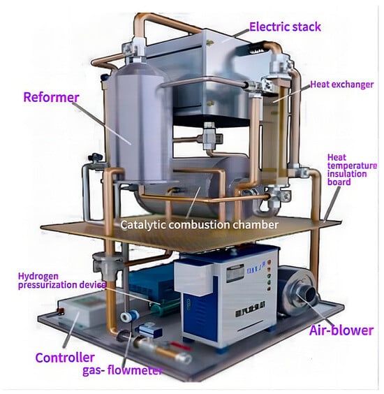
Figure 1.
Architecture diagram of the SOFC system.

Table 1.
The SOFC system’s parameter settings.
When the SOFC system is in operation, water and a portion of the hydrogen in the cold box are introduced into the reforming chamber after preheating in the evaporator, while another portion of the hydrogen enters the reforming combustion chamber and undergoes a combustion reaction with the air, thus providing continuous high temperature conditions for the subsequent reforming reaction. In the hot box, the air–exhaust heat exchanger exchanges the high temperature exhaust gas from the exhaust combustion chamber with the cathode’s cold air introduced into the system, so that the temperature of the cathode’s air rises to about 600 °C after the first heat exchange. The fuel–air heat exchanger exchanges the reformed high-temperature fuel gas with the cathode’s air after the first heat exchange to reduce the temperature difference between the anode’s gas and the cathode’s air.
In order to maximize the energy output and reduce the overall cost of the system, the SOFC system has adopted an innovative thermal management strategy, including combined heat and power (CHP) technology, to recover the waste heat generated by the SOFC stack and tail gas combustion chamber for heating or other industrial processes. In addition, the system design emphasizes modularity and expansibility, and is easy to maintain and upgrade. The SOFC system not only improves energy efficiency but also reduces the dependence on fossil fuels, which is consistent with the goal of low-carbon energy policies. By using pure hydrogen or natural gas as fuel, the system reduces harmful emissions and contributes to sustainable industrial development.
Figure 2 shows the configuration of the SOFC system used in this study. An SOFC system with 3 kW of power runs in parallel with the hot water system, and the stack is connected with the corresponding 1 kW tail gas combustion chamber. The heat exchanger can be categorized into two parts, which are used for preheating cold air and fuel–air temperature equalization before their entrance into the stack. Prior to conducting the experiment, the measuring devices and monitoring system underwent a thorough inspection and recalibration to verify the accuracy and reliability of the measurements.
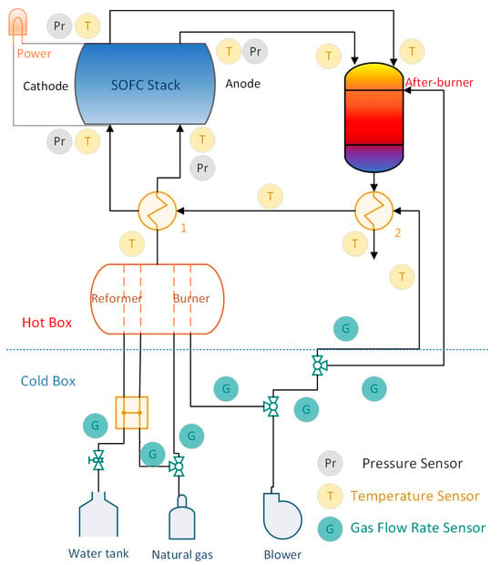
Figure 2.
Block diagram of the SOFC system.
2.2. Dataset
The original dataset used in this study consisted of 82 variables that collected 662,327 observations from the real-time monitoring system at 1-s intervals, based on the data of five recent experiments [35,36]. In this process, the temperature, flow rate, and power consumption are monitored at 1 s intervals utilizing a PT 100 thermometer with a precision of 0.2%, an electronic load with an accuracy of ±0.2%, and a flow meter with an accuracy of ±0.5%.
There are too many variables in the original dataset, shown in Table 2. Therefore, the data’s dimensionality was reduced using the correlation variable method and PCA (2.3 (3)), to obtain 12 variables (Tafterburner, feed CH4 PV, burner CH4 PV, stack air PV, feed water pump SV, premix air PV, burner air PV, I, TC22, TC3, TC2, and TC10) as the input variables and three variables (stack temperature, voltage, and temperature) as the predicted output variables; all are shown in Table 3. Meanwhile, Table 3 gives the unit of each variable, the method of obtaining it, and the type of variable it is in this study.

Table 2.
Original variables and their interpretation.

Table 3.
Input and output variables.
The power consumption of parasitic components was not included in this study. In this study, the power consumption data (kW), temperature data (°C), and airflow velocity (NL/min) of the SOFC system and its corresponding combustion chamber and hot water system were measured. At the same time, the water demand data at 1 h intervals were obtained from the water tank’s flow sensor and combined into the dataset.
2.3. Data Processing
- (1)
- General
Figure 3 illustrates a flow chart of the research, outlining the process of predicting the performance of the SOFC system. The appropriate input variables were identified through principal component analysis (PCA), followed by an analysis of the system’s performance and its associated variables. In terms of predictive modeling, an initial multiple linear regression (MLR I) model was established to quantitatively assess the factors influencing the system’s performance. If the assumptions of the MLR model were not met, a second MLR model (MLR II) was developed by incorporating additional variables to enhance the predictions’ accuracy. Subsequently, the optimal structure of a neural network model was determined using the same variables as the MLR model to capture any nonlinear relationships between the response and explanatory variables. Finally, the model demonstrating strong predictive capabilities was utilized as the benchmark for predicting the thermoelectric performance of the SOFC system.
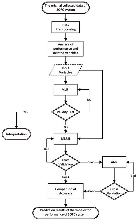
Figure 3.
Flow chart of the research.
- (2)
- Preliminary data processing
For the cogeneration of the SOFC system, we can use Equation (3) to calculate the total thermal energy output () and electric energy output () at an interval of 1 h, combining the temperature difference between the fuel inlet and outlet (, ), the increase in the temperature of the water (, ), the unit conversion factor (, ), and the rate of fuel flowing (, ) through the SOFC. The subscript “”represents different cogeneration units. The molar mass () and specific heat capacity () of water were assumed to be constant under the operating conditions, and “” and “” are the start and end data of the corresponding period.
Analysis of the performance and predictive modeling of the SOFC system were carried out by averaging the scale datasets of each time and every hour. Only when the cogeneration mode of the SOFC system was in the start-up state, we could carry out time-weighted averages for intensive variables such as fuel, the air flow rate, and temperature. For thermoelectric output variables, whether the system was running or not, these should be continuously accumulated to calculate the overall thermoelectric output. The time series of changes, the system’s operation mode, the frequency distribution, and basic statistical data of the related variables were analyzed for predictive modeling of the performance and interpretation of the results.
Given the different dimensions of the original data, we first used the mapminmax function to normalize the data, as shown in Equation (4), where represents the raw data, represents the minimum value in the raw data, represents the maximum value in the raw data, and and represent the normalized maximum and minimum values, respectively.
- (3)
- PCA method
The method of principal component analysis (PCA) offers a robust mathematical structure for pinpointing the principal trends within datasets with multiple variables. By detecting inter-variable correlations within the defined state space, PCA facilitates the discovery of a new coordinate framework that aligns with the greatest variations in the dataset. This alignment enables the dismissal of subsidiary dimensions while preserving the dataset’s fundamental structure. The intricacies of the PCA’s process of reducing the dimensionality have been previously detailed in [37]. In this discussion, the essence of PCA is succinctly revisited, and a comprehensive analysis of how preprocessing and post-processing of the data influence PCA’s effectiveness will be undertaken.
The PCA methodology involves mapping n instances of attributes onto an dimensional matrix , with each row capturing a distinct instance of the attributes . In the context of the combustion-related examples addressed within this study, the attributes in the matrix correspond to temperature measurements and species’ mass fraction data. The PCA technique transforms through basic rotation, which is computed via decomposition of the eigenvalues of the dimensional covariance matrix.
wherein represents the eigenvectors and signifies the eigenvalues derived from . The reoriented basis, constituted by the eigenvectors , can be condensed to encapsulate primarily the most dynamic directions (the specific columns of that correspond to the most substantial eigenvalues in ). This results in the formation of a rectangular matrix , onto which the initial dataset is mapped to generate the principal components (PCs), denoted .
Equation (5) can be reversed to yield a reconstructed approximation of the initial sample with the dimensions .
Equation (6) facilitates a linear method of reconstruction. The fundamental linear nature of PCA poses a significant limitation when applied to highly nonlinear phenomena such as combustion. Nonetheless, this constraint can be mitigated to some extent through the use of localized PCA techniques. In contrast, nonlinear methods of reconstruction (Equation (5)) could yield more precise correlations between and .
2.4. Calculation of the System’s Performance
Through data preprocessing, it was found that the remaining key variables could be used to calculate the performance of the SOFC system. The efficiency () of the SOFC system was calculated by using the fuel consumption () of the SOFC, the power () generated, and the increasing trend of the cooling water’s temperature () generated by the data at 1-h intervals, as shown in Equation (8), where the subscript “” is the observed data variable. The formula for calculating the efficiency of the SOFC system is as follows:
Among these, if is , is the low calorific value of hydrogen, and the value is 241.83 kJ mol−1. Only the efficiency () of the SOFC system can be calculated by Equation (8), and fuel consumption is used as the denominator. Given the performance parameters corresponding to the cooling water tank, Equation (8) can be applied to obtain the heating efficiency of the SOFC system. If the electric power required by the external load is given, the power generating efficiency of the SOFC system can be calculated by Equation (8).
2.5. Predictive Models of Performance
- (1)
- MLR
MLR is a model where the dependent variable () is determined by a linear combination of multiple independent variables or explanatory variables (), as depicted in Equation (9).
The parameters in Equation (9) are computed through the OLS technique, and it identifies optimal solution of the residual sum of squares () by Equation (10); represents the predicted response variable, and denotes the model’s residual.
In order for the multiple regression (MR) model to achieve the best linear unbiased estimation (BLUE), certain assumptions must be met. These include: (1) the residuals should follow a normal distribution with an expected value of zero; (2) nonautocorrelation, i.e., the residuals should not be correlated with each other; (3) homoscedasticity, i.e., each residual should have the same finite variance; and (4) among the explanatory variables, there should be no exact multicollinearity. If the assumptions of nonautocorrelation and homoscedasticity are violated, the estimation’s coefficients will remain consistent and unbiased. However, the estimated variance of the OLS estimator will be biased, leading to unreliable results in T tests, F tests, and the determination coefficient (R). The MLR model should adhere to the “saving principle” and strive for a good fit, that is, the R standard should be greatly adjusted and it should be consistent with relevant theories.
- (2)
- ANN
ANN is a computational method used in numerical analysis to estimate the relationship between input variables and output variables. The neural network of MLP comprises neurons, synapses, and layers. The input and output layers comprise every independent variable, which function as the neurons, and every respective corresponding dependent variable, and additional concealed layers containing different quantities of neurons can be inserted between them. A deep neural network (DNN), which has multiple hidden layers, is an artificial neural network. In both the input and hidden layers, a bias term is incorporated, and the synapses are exclusively linked to the subsequent layer. For neurons and a hidden layer, the relationship between the explanatory variable () and the predicted response variable () can be expressed using Equation (11) involving weight parameters ( and ), constant terms ( and ), and an activation function () that is differentiable, and it is monotonically increasing. In this research, the hyperbolic tangent function was utilized as the activation function.
Regression analysis determines the weight parameters of ANN model through finding the optimal solution, minimizing the , as defined in Equation (7). We used the BP algorithm as outlined in Equation (12) to update the parameters until the objective function, represented by the RSS, reached a specified convergence threshold. Here, the variable “” denotes the learning rate, and “” signifies the current iteration step.
In this study, we improved the limitations of the backpropagation (BP) algorithm through the application of the gradient descent method. These limitations include sensitivity to the initial weights and abnormal data points, the possibility of staying at the local minimum, overfitting the training data, and slow calculation efficiency. In order to overcome these problems, the elastic propagation (Rprop) algorithm including a backtracking mechanism and the DBN pretraining technology was adopted to construct the neural network model. The Rprop algorithm is considered to be one of the fastest and most stable methods for updating weights. It is different from the traditional BP algorithm because it adjusts the learning rate for each parameter in each iteration, which is based on whether a partial derivative sign of a certain weight has changed in two successive iterations. In addition, the backtracking mechanism is a powerful technology which helps to avoid crossing the local minimum by reducing the weight’s updated amount when the symbol changes and retreating to the previous iteration when necessary. On the other hand, the data bank network (DBN) sets the initial values for the weights through an unsupervised pretraining process, which is regarded as a strategy to prevent the optimization process from falling into the local minimum. This kind of pretraining has been found to promote regularization and to initialize the parameters of the deep neural network (DNN) to a region close to the ideal local minimum, thus helping to improve the ability for generalization in global supervised learning. In order to verify the external predictive ability of the model and exclude the possibility of overfitting, this study used the cross-validation (CV) technique. When determining the optimal structure of the neural network and estimating the weight parameters, several different initial weights were tested.
2.6. Evaluation of Predictive Accuracy
The evaluation of the predictive accuracy of ANN and MLR models was conducted through the use of the normalized mean error () and the normalized root mean square error coefficient (). and were derived through dividing the mean absolute error () and root mean square error () by the response variables’ () average value, thereby rendering both indices independent of variable scales. serves as an indicator of the overall deviation of predicted values, while assesses the mean standard error of predicted values, as delineated in Equations (13) and (14), correspondingly. In these formulas, denotes the measured value of the j-th variable, represents the predicted value of the j-th variable, and signifies the total number of observations. A nonzero value indicates that the total error will not be offset. Equation (15) utilizes MAE to compare the predictions’ errors with those observed in other studies.
3. Results
This experiment was completed on the MATLAB software platform. The computer for analysis was the Windows 11 system, the central processor was an Intel CORE i5, the memory capacity was 16 G, and the hard disk capacity was 512 G.
3.1. Statistical Results of Thermoelectric Performance Variables
When evaluating the cogeneration performance of the SOFC system, the combined heat and power efficiency (CHP) of the SOFC system was 1.85 according to Equation (6). In a set evaluation period, the power consumption of the system per hour was 1 kWh, which only considered the power consumption of the SOFC system when generating electricity and heating at the same time, and did not include the power consumption of any auxiliary equipment such as the circulating pump. In contrast, under the standard test conditions of a fuel input temperature (FIT) of 650 °C and an exhaust temperature (ET) of 60 °C, the rated electrical efficiency (EE) of the SOFC system was 50%, while the thermal recovery efficiency (TRE) was 30%. Table 4 summarizes the performance parameters (TPP) of the SOFC system and the average value of heating water consumed for five experiments.

Table 4.
Performance and operation of the combined heat and power supply of the SOFC system each time.
Figure 4 shows the peak water temperature, quantity of heating water, median power, running time, and so on of the five experiments. Among them, the average power generated was 785 W. The average amount of heating water was 3140 L, the average peak temperature of water was 66.6 , and the average running time was 395.6 h. There was a certain relationship between both the peak water temperature and water consumption, and the season in which the experiment was carried out. For example, the water consumption in winter is relatively small and the peak water temperature is low. In summer, the water consumption is greater and the peak water temperature is higher. This can explain the relationship between water consumption and peak temperature, but in order to simplify the research, this study did not consider the seasonal influence on the SOFC system for the time being.
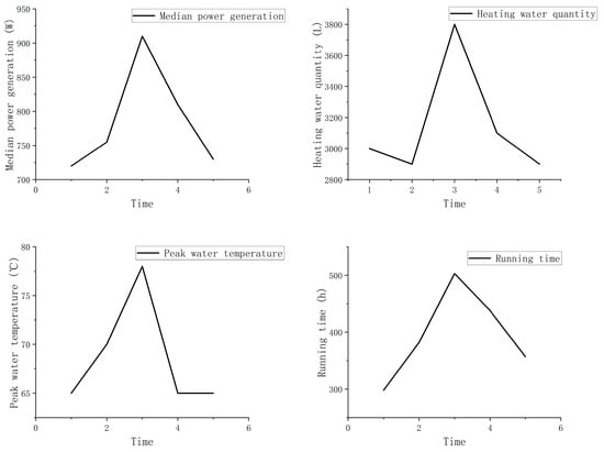
Figure 4.
Sequential changes in temperature and the quantity of water used for heating each time.
3.2. Analysis of Related Variables Affecting the System’s Performance
According to the operation data of the SOFC system in Figure 4 above, combined with the detailed flow rate of air supply at multiple positions, temperature, air pressure and load parameters of the system, correlation analysis of the variables was carried out, as shown in Figure 5. The process of the correlation analysis of the variables was as follows.
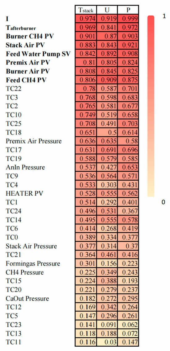
Figure 5.
Correlation diagram of the variables.
- (1)
- According to the operating data of the SOFC system for five experiments, shown in Figure 4, we extracted the parameters of the fuel/air flow rate and fuel/air pressure of multiple components during each operation, as well as the load power, the stack’s temperature, the combustion chamber’s temperature, and the change in the cooling water’s temperature.
- (2)
- We drew a chart of the fluctuation trend of each parameter according to the time series (the trend chart has been omitted in this article) and preprocessed the data. The standard deviation method was used to eliminate outliers in during preprocessing, and the nearest neighbor interpolation method was used for missing values.
- (3)
- We carried out a correlation analysis of the data, sorted out the variables with large correlations and the variables with small correlations, and prepared for reducing the data’s dimensionality.
- (4)
- Data normalization was realized by minimum–maximum normalization to obtain data that could be used for reducing the data’s dimensionality.
- (5)
- Principal component analysis (PCA) was used to reduce the dimensions; the specific method is shown in Equations (5)–(7).
Through the steps above, a diagram of the variables’ correlation, as shown in Figure 5, was obtained. See the Table 2 for specific explanations of each variable.
The fuel utilization rate, the stack’s current, and the temperature of the heating water of the SOFC system are necessary conditions for understanding the system’s operating characteristics and establishing a predictive model of the thermoelectric performance. Figure 6 shows the voltage, current, and power curves of five experiments caused by factors such as the fuel’s flow rate and fluctuations in the water temperature. The rapid cooling of water expressed the process of changing the water, and the volume of water changed was 100 L each time. Although the volatility was high at this time, the process of exchanging the water was ignored in this study.
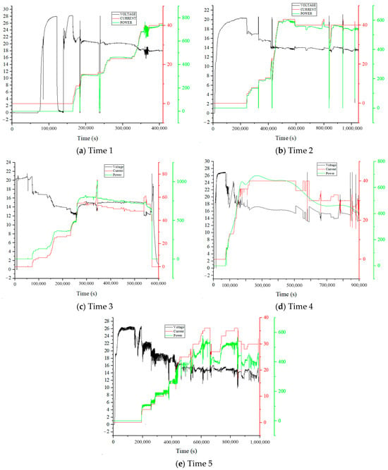
Figure 6.
Waveforms of voltage, current, and power in five experiments.
Through an analysis of Figure 6, it was found that there were differences in the duration, and the range of variation in the voltage and power during each operation of the SOFC system, which were mainly due to factors such as the inconsistent state of the used stack and the external environment.
According to the “on” or “off” state of the switch, the value of each BOP and component of the stack was set to 1 or 0, and the values of eight system subcomponents were added to obtain the parameters of the system’s components that operated together every minute, that is, an integer between 0 and 8. This parameter was named “NK” in this study, and NK represents the average number of the system’s subcomponents running at full load every hour. When making a predictive model of the performance, we used the average value of NK as one of the process’s variables.
3.3. Quantitative Analysis of the Variables of Interest
Table 5 is the tabular form of Figure 5. Table 5 shows the Pearson correlation coefficients (PCCs) which mainly affected the performance and variables of the SOFC system. The closer a PCC’s value is to 1, the stronger the correlation of the two variables.

Table 5.
Correlation matrix of the key variables of the thermoelectric performance of the SOFC system.
For the sake of quantitatively analyzing the influencing factors of the thermal and electrical performance of SOFC systems, a MLR model that demonstrated the statistical significance was established, namely Equation (16), after evaluating different combinations of functional forms and explanatory variables, including logarithmic, polynomial, and reciprocal functions. The effectiveness and predictive accuracy of the model were evaluated on the basis of the standards described in Section 2.5 and Section 2.6. To eliminate the uncertainty caused by the system’s startup and shutdown, outliers were excluded from the original 1978 datasets, accounting for 3.7%, including 12 Boolean data columns. Based on value of PCC, we chose the top 12 most correlated observed variables to model.
On the basis of engineering theory, we introduced four core variables that can affect the thermoelectric performance of a SOFC system into the model: external load (EL), the fuel’s flow rate (FLR), water consumption (UUV), and water temperature (WT). When the external load ran within the available power range of the SOFC, the thermoelectric performance of the SOFC system was improved under the conditions of high FLR and high UUV and WT. The linear combination of the four core variables and three outputs of the system could explain the power generation performance of the SOFC system, and all variables, including constant terms, demonstrated statistical significance, as shown in Table 6; b1–b9 are constant coefficients.

Table 6.
The MLR model’s coefficients with statistical significance.
Identifying the variables that exerted a substantial influence on performance through correlation analysis posed challenges due to its limitations in capturing the effects of other variables. Correlation serves as a measure of the linear association between two variables, but it does not account for the influence of other variables that are held constant. According to the results above, we could see which variables had a significant impact on performance, so there was no need to add variables to build the MLR II model.
3.4. Results of the Predictive Model of the SOFC System’s Performance
Ongoing research initiatives are being conducted utilizing “Matlab”, which is an open-source programming language for graphical and statistical computations.
3.4.1. MLR
To construct a MLR model for forecasting the thermoelectric efficiency of solid oxide fuel cell (SOFC) systems, the following variables were also implicated, according to Equation (14): (1) the methane inlet’s flow rate, the combustion chamber’s methane flow rate, the stack’s air flow rate, the combustion chamber’s air flow rate, the air flow rate, the flow rate of deionized water, the current, and the combustion chamber’s temperature, etc., and (2) consumption of cooling water and change in temperature. These variables were selected according to the results of the principal component analysis and whether the NRMSE of the test set was improved through cross-validation. According to the analytical model of the factors influencing performance, the minute-level predictive model of the performance in power generation was the final model. We defined MLRX (X = 1, 2, 3, 4, 5) to represent the model of five training rounds. Table 7 shows the five MLR models’ results after cross-validation, and the results in the table are based on the whole process, with both training and testing phases being included. The best prediction for each output variable in the table has been bolded. Figure 7 shows the comparison between the predicted value of MLR model and the measured value, in which red represents the measured data, blue represents the training data, and purple represents the test data. It can be seen that the predicted value is basically consistent with the measured value, indicating that the predictive model is reliable. By averaging, applying the final MLR model, the prediction’s accuracy in terms of NRMSE improved to 1.89%.

Table 7.
Minute-level predictive accuracy of the MLR model of performance obtained by cross-validation.
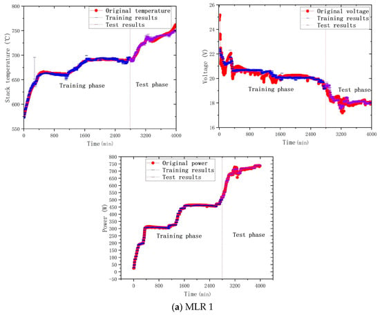
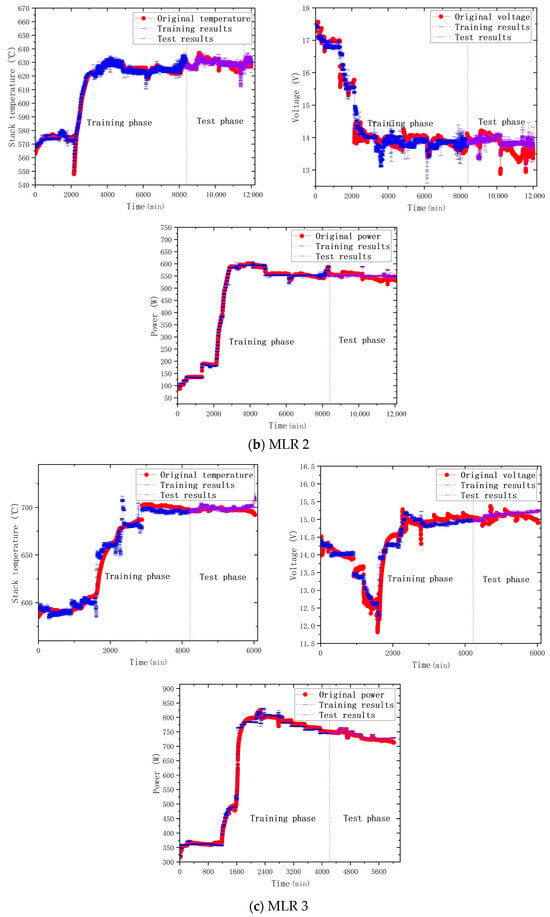
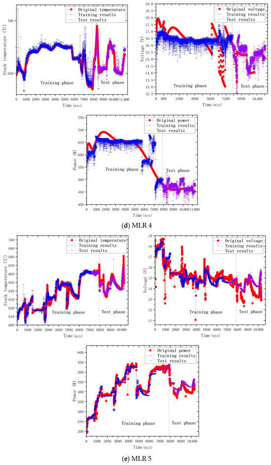
Figure 7.
Comparison between the MLR’s prediction and the original data.
In order to visualize the predicted effects more visually using images, Figure 8 shows the residual analysis of MLR for each round. As can be seen from Figure 8, the errors of MLR1 in predicting the temperature, voltage, and power of the stack were all within 5%, and a good predictive effect was achieved. Although the error of MLR2 for predicting the temperature, voltage, and power of the stack fluctuated greatly, the overall predictive error was kept within 10%, which could basically realize the prediction and tracking of the target value. There were some errors in the predictions of temperature, voltage, and power of MLR3, but the overall error was not high. The predictive error of MLR4 regarding the temperature, voltage, and power of the stack was large, and the overall error exceeded 20%, so the predictive effect was not ideal, which will be explained in Section 4. The predictive error of MLR5 for the temperature, voltage, and power of the stack fluctuated greatly, and the predictive effect was average.
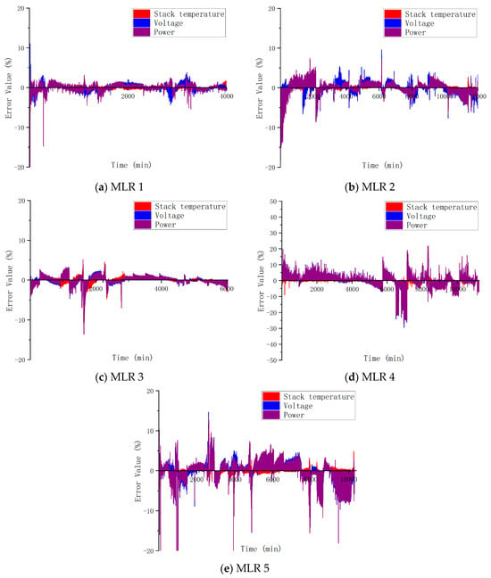
Figure 8.
Residual analysis for testing the MLR model’s hypothesis.
3.4.2. ANN
In this section, the same input variables as those in the MLR model in Section 3.4.1 were selected, and the predicted values of five corresponding output variables were obtained through fitting and training the neural network. Simultaneously, we established TimeX (where X ranged from 1 to 5) to align with MLRX (where X ranged from 1 to 5). By changing the number of hidden layers and neurons by trial and error, the optimal structure of the ANN model (3 hidden layers and 10 neurons) was determined, so that the best predictive value could be obtained without overfitting. Table 8 shows the minute-level predictive accuracy of performance by cross-validation of the neural network model, and the best predictions for each output variable are bolded in the table. Figure 9 shows the comparison between the predicted values of the ANN model and the measured values, where red, blue and purple represent the measured data, the training data, and the test data, respectively. The experimental results showed that the predicted values of ANN were basically consistent with the measured values, and the MAE and RMSE of the three output variables were within the acceptable range, which showed that it is reliable for predicting the thermoelectric output of the SOFC system. And by averaging, the predictive accuracy in terms of NRMSE improved to 0.66%.

Table 8.
Minute-level predictive accuracy of performance for the ANN model obtained by cross-validation.
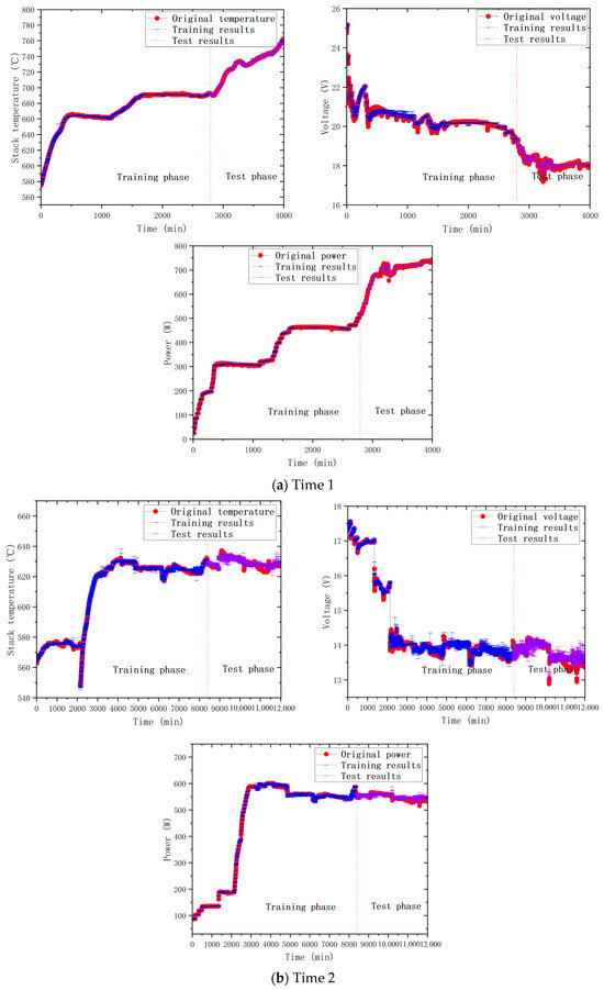
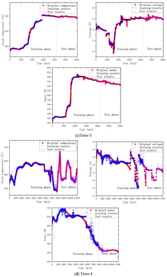
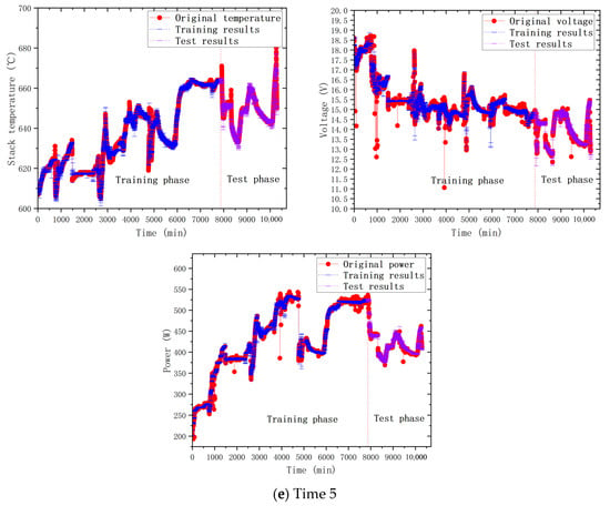
Figure 9.
Comparison between ANN’s predictions and the original data.
3.4.3. Comparison of the Predictive Accuracy
In a comparison of the predictive accuracy of these two prediction methods for the same output variable, it was clearly seen that the predictive accuracy of the ANN model was better than that of the MLR model for the five groups of results. Especially in the fourth group, it was obvious that the MAE, NME, and NRMSE of the MLR model were about 0.56, 3.51, and 5.20, respectively, but for the ANN model, they reduced to 0.16, 0.97, and 1.50, respectively. In terms of predicted power, the MAE, NME, and NRMSE of the MLR model were about 20.99, 3.64, and 5.46, respectively, but they reduced to 5.98, 1.04, and 1.67 in the ANN model. Generally speaking, in terms of the stack’s temperature, the MAE value, NME value, and NEMSE value of the ANN model were kept to 0.7–1.2, 0.1, and 0.3, respectively, with a small error. The MAE value, NME value, and NRMSE value of the MLR model remained at 0.3–0.7 and 0.3–1.0. From the above, it can be seen that the predictive accuracy of the ANN model was significantly higher than that of the MLR model. This suggests a more complicated association between the independent and dependent variables that exceeds the explanatory capacity of the current MLR framework. While the predictive accuracy of the MLR was is inferior to that of the ANN model, the predictive accuracy of the MLR model for the SOFC’s thermoelectric performance was still high.
4. Discussion
By analyzing the model coefficients in Table 6, it can be found that the parameters in the SOFC system, such as methane inlet’s flow rate, the flow rate of methane in the combustion chamber, the stack’s air flow rate, the combustion chamber’s air flow rate, the air flow rate, the flow rate of deionized water, the current, and the combustion chamber’s temperature, had significant effects on the stack’s temperature, voltage, and power output. In different models, the methane inlet’s flow rate, the flow rate of methane in the combustion chamber, the stack’s air flow rate, and the combustion chamber’s air flow rate had negative effects on the combustion chamber’s temperature. Reducing these flow rates is beneficial for reducing the stack’s temperature and realize the control of the temperature of the SOFC’s stack. The air flow rate, the flow rate of deionized water, and the combustion chamber’s temperature had positive effects on the stack’s temperature, and controlling these parameters is beneficial for controlling the stack’s temperature. However, the methane inlet’s flow rate, the combustion chamber’s methane flow rate, and the stack’s air flow rate had positive effects on voltage in most models, and increasing these flow rates appropriately would be beneficial for improving the voltage output. The air flow rate, the flow rate of deionized water, and the current had little influence on the voltage and had different effects. The direction and magnitude of the influence of air velocity, the current, and the combustion chamber’s temperature were different in different models, which indicates that their relationship with the power output is complex and may be influenced by other parameters and working conditions of the system. The key parameters above have an important influence on the temperature, voltage, and power of the stack, and the specific situation may need to be further studied in combination with specific working conditions. These analytical results provide theoretical guidance for optimization of the SOFC system’s operation and may help to improve the performance and efficiency of the stack by fine-tuning various parameters.
Further discussing the correlations between the variables, Table 9 lists the combustion chamber’s temperature, the stack’s temperature, and power at different flow rates of methane in this study. It can be observed that as the methane’s flow rate increases, the changes in the other variables are not linear, especially the change in power. This is because a change in quantity will inevitably cause changes in other variables, and a variable is influenced by many factors. The variables do not have a simple linear relationship with each other. This is the dynamic nonlinearity within the SOFC system. Therefore, machine learning methods are needed. This can help us accurately predict the changes in the output of complex systems.

Table 9.
Values of selected variables at different flow rates of methane.
In addition, from the results of the two different forecasting methods, MLR and ANN, as seen in Table 7 and Table 8, the accuracy of the predicted voltage was higher than the accuracy of predicted power. This is because the power is the product of the current and the voltage, and the current is larger, so the error of the output power will become larger. Moreover, through the results in Section 3.4, it was found that regardless of the method, the fourth group of data predicted significantly worse results than the other groups. This is because the machine malfunctioned when carrying out the experiments for that group, making the actual values obtained somewhat wrong. This is why the predictions were not as good as they could have been. Nonetheless, the predictions were still roughly in line with the trend of the measured data. This shows that the prediction models built by the two methods above with the wrong data still have a certain degree of accuracy, indicating their robustness.
The prediction models built by both methods used in this study had high average predictive accuracy, with a mean NRMSE of 1.89% for the MLR model and 0.66% for the ANN model. In comparison with the other prediction methods available, the GA-BP algorithm model had the lowest predictive accuracy of 1% [7], and the ANN model in this study was significantly better than this. If the fourth set of data with errors is removed, then the predictive accuracy in terms of NRMSE for the ANN model was reduced to less than 0.5%. Compared with to the LSTM method used in [6], the ANN method used in this study was simpler and more efficient, with similar predictive accuracy. In addition, compared with the BPNN method [38], the advantages of the two methods used in this study were more obvious [38]. Overall, the two models used in this study, the ANN model and the MLR model, not only had high predictive accuracy but were also simpler and more efficient than other prediction models that have been used.
Meanwhile, in this study, temperature, flow rate, and power consumption were monitored at 1 s intervals utilizing a PT 100 thermometer with a precision of 0.2%, an electronic load with an accuracy of ±0.2%, and a flow meter with an accuracy of ±0.5%. These measuring instruments had a certain amount of error anyway, which made this study have a certain amount of uncertainty. In order to analyze this, Equation (17) was used to calculate the total uncertainty of this study [39], where , , and represent the error of each measuring instrument, respectively. and represents the total uncertainty of this study. After calculation, it was found that the uncertainty of this study was 0.57%.
5. Conclusions
By integrating field monitoring data and using the techniques exploratory data analysis, the thermoelectric performance of a single SOFC system (comprising a combustion chamber and a cooling water supply subsystem) was computed, and the system’s operating patterns were determined on the basis of five instances of the system’s operating data. The MLR model, demonstrating statistical significance, reliably elucidated the quantitative impacts of the influencing variables on the system’s performance, providing logical grounds for analyzing variations in the system’s performance, such as identifying the key factors affecting the characteristics of the system’s output through an analysis of correlated variables. The MLR (1.89%) and ANN (0.66%) models developed in this study exhibited satisfactory precision in predicting the minute-level thermoelectric performance of the system, serving as references for real-time monitoring of the SOFC system’s performance. And it can provide guidance for improving the thermoelectric performance of SOFC systems, so as to contribute to the cause of sustainable development. This study underscores the advantage of MLR in quantitatively analyzing performance-influencing factors, while also demonstrating the superior predictive capability of ANN in forecasting the system’s performance. Although this study focused on SOFC systems, the same methodology and procedures can be extended to develop predictive models for other types of energy facilities and corresponding time periods.
Author Contributions
Conceptualization and methodology, X.W. and X.L.; validation, D.Z.; formal analysis, M.L.; writing—original draft preparation, M.L.; writing—review and editing, M.L., D.Z. and Y.L.; supervision, X.W. and X.L.; project administration, X.L.; funding acquisition, X.W. and X.L. All authors have read and agreed to the published version of the manuscript.
Funding
This research was funded by the National Natural Science Foundation of China (grant nos. 62203204 and U2066202), Jiangxi Provincial Natural Science Foundation (grant nos. 20232BAB202028 and 20212BAB212013), China Postdoctoral Science Foundation Funded Project (Grant no. 2023M732387), and Belt and Road Joint Laboratory on Measurement and Control Technology Fund (No. mct202102).
Data Availability Statement
The original contributions presented in the study are included in the article, further inquiries can be directed to the corresponding author.
Acknowledgments
The authors would like to thank the National Natural Science Foundation of China (62203204, U2066202), Jiangxi Provincial Natural Science Foundation (20232BAB202028), Belt and Road Joint Laboratory on Measurement and Control Technology Fund (mct202102) and the College Students’ Innovative Entrepreneurial Training Plan Program of China (grant No. 202210403096 and No. 202210403098).
Conflicts of Interest
The authors declare no conflicts of interest.
References
- Vinchhi, P.; Khandla, M.; Chaudhary, K.; Pati, R. Recent advances on electrolyte materials for SOFC: A review. Inorg. Chem. Commun. 2023, 152, 110724. [Google Scholar] [CrossRef]
- Wu, X.; Xu, Y.; Peng, J.; Xia, Z.; Kupecki, J.; Li, X. Novel Hybrid Modeling and Analysis Method for Steam Reforming Solid Oxide Fuel Cell System Multifault Degradation Fusion Assessment. ACS Omega 2023, 8, 36876–36892. [Google Scholar] [CrossRef] [PubMed]
- Shang, Z.; Hossain, M.M.; Wycisk, R.; Pintauro, P.N. Poly (phenylene sulfonic acid)-expanded polytetrafluoroethylene composite membrane for low relative humidity operation in hydrogen fuel cells. J. Power Sources 2022, 535, 231375. [Google Scholar] [CrossRef]
- Rezk, H.; Olabi, A.; Abdelkareem, M.A.; Maghrabie, H.M.; Sayed, E.T. Fuzzy Modelling and Optimization of Yeast-MFC for Simultaneous Wastewater Treatment and Electrical Energy Production. Sustainability 2023, 15, 1878. [Google Scholar] [CrossRef]
- Kim, J.; Kim, Y.; Song, H. Development of a new configuration and optimization of the 5-kW class energy conversion system combining a solid oxide fuel cell and internal combustion engine using a spark-assisted ignition. Energy Convers. Manag. 2023, 291, 117329. [Google Scholar] [CrossRef]
- Rao, M.M.; Wang, L.; Chen, C.T.; Xiong, K.; Li, M.F.; Chen, Z.P.; Dong, J.B.; Xu, J.L.; Li, X. Data-Driven State Prediction and Analysis of SOFC System Based on Deep Learning Method. Energies 2022, 15, 3099. [Google Scholar] [CrossRef]
- Zhang, D.H.; Hu, J.G.; Zhao, W.; Lai, M.L.; Gao, Z.L.; Wu, X.L. A Single-Stack Output Power Prediction Method for High-Power, Multi-Stack SOFC System Requirements. Inorganics 2023, 11, 474. [Google Scholar] [CrossRef]
- Xiong, X.Y.; Xue, Z.Z.; Wu, X.; Wu, Y.F.; Peng, S.P. Modelling and flow rate control methods for anode tail gas circulation intake system at SOFC. Int. J. Hydrogen Energy 2022, 47, 16201–16213. [Google Scholar] [CrossRef]
- Williams, N.J.; Osborne, C.; Seymour, I.D.; Bazant, M.Z.; Skinner, S.J. Application of finite Gaussian process distribution of relaxation times on SOFC electrodes. Electrochem. Commun. 2023, 149, 107458. [Google Scholar] [CrossRef]
- Xiong, X.; Liang, K.; Ma, G.; Ba, L. Three-dimensional multi-physics modelling and structural optimization of SOFC large-scale stack and stack tower. Int. J. Hydrogen Energy 2023, 48, 2742–2761. [Google Scholar] [CrossRef]
- Liang, W.; Yu, Z.; Bian, F.; Wu, H.; Zhang, K.; Ji, S.; Cui, B. Techno-economic-environmental analysis and optimization of biomass-based SOFC poly-generation system. Energy 2023, 285, 129410. [Google Scholar] [CrossRef]
- Alsarraf, J.; Alnaqi, A.A.; Al-Rashed, A.A.A.A. Thermodynamic modeling and exergy investigation of a hydrogen-based integrated system consisting of SOFC and CO2 capture option. Int. J. Hydrogen Energy 2022, 47, 26654–26664. [Google Scholar] [CrossRef]
- Singh, U.R.; Bhogilla, S. Exergy analysis of reversible sofc coupled with organic Rankine cycle and hydrogen storage for renewable energy storage. Int. J. Hydrogen Energy 2023, 48, 39169–39181. [Google Scholar] [CrossRef]
- Cheng, J.; Lavery, R.; McCallum, C.S.; Morgan, K.; Doran, J.; Wu, C.; Sun, K.; Rooney, D.W. Crossflow flat solid oxide fuel cell (SOFC) semi-empirical modeling and the multi-fuel property based on a commercial 700 W stack. Fuel 2024, 358, 130172. [Google Scholar] [CrossRef]
- Omer, A.; Rahimipetroudi, I.; Rashid, K.; Yang, J.B.; Dong, S.K. Design and performance optimization of a direct ammonia planar solid oxide fuel cell for high electrical efficiency. J. Power Sources 2023, 573, 233135. [Google Scholar] [CrossRef]
- Wu, X.J.; Huang, Q.; Zhu, X.J. Thermal modeling of a solid oxide fuel cell and micro gas turbine hybrid power system based on modified LS-SVM. Int. J. Hydrogen Energy 2011, 36, 885–892. [Google Scholar] [CrossRef]
- Kang, Y.W.; Li, J.; Cao, G.Y.; Tu, H.Y.; Li, J.; Yang, J. Dynamic temperature modeling of an SOFC using least squares support vector machines. J. Power Sources 2008, 179, 683–692. [Google Scholar] [CrossRef]
- Zhang, Y.Y.; Huang, J.D.; Zhang, Y. A Predictive Model of SOFC Thermal Management Based on LS-SVM. Appl. Mech. Mater. 2014, 538, 274–277. [Google Scholar] [CrossRef]
- Ding, C.; Xia, Y.; Yuan, Z.; Yang, H.; Fu, J.; Chen, Z. Performance prediction for a fuel cell air compressor based on the combination of backpropagation neural network optimized by genetic algorithm (GA-BP) and support vector machine (SVM) algorithms. Therm. Sci. Eng. Prog. 2023, 44, 102070. [Google Scholar] [CrossRef]
- Sani, M.; Piffard, M.; Heiries, V. A Hybrid Diagnosis for Gas Starvation Faults in Proton Exchange Membrane Fuel Cells. In Proceedings of the 2023 62nd IEEE Conference on Decision and Control (CDC), Singapore, 13–15 December 2023; pp. 5837–5844. [Google Scholar]
- Wang, L.J.; Zhang, H.S.; Weng, S.L. Modeling and simulation of solid oxide fuel cell based on the volume-resistance characteristic modeling technique. J. Power Sources 2008, 177, 579–589. [Google Scholar] [CrossRef]
- Wu, X.J.; Zhu, X.J.; Cao, G.Y.; Tu, H.Y. Dynamic modeling of SOFC based on a T-S fuzzy model. Simul. Model. Pract. Theory 2008, 16, 494–504. [Google Scholar] [CrossRef]
- Quan, R.; Liang, W.; Wang, J.; Li, X.R.; Chang, Y. An enhanced fault diagnosis method for fuel cell system using a kernel extreme learning machine optimized with improved sparrow search algorithm. Int. J. Hydrogen Energy 2024, 50, 1184–1196. [Google Scholar] [CrossRef]
- Liu, X.; Jia, X.; Wei, Y.; Wei, L.; Zhou, Y. Comparison of Degradation Prediction Methods for Proton Exchange Membrane Fuel Cell. In Proceedings of the 2023 Prognostics and Health Management Conference (PHM), Big Sky, MT, USA, 4–11 March 2023; pp. 152–158. [Google Scholar]
- Yu, Y.; Chen, S. Numerical study and prediction of water transfer in gas diffusion layer of proton exchange membrane fuel cells under vibrating conditions. Int. J. Energy Res. 2022, 46, 18781–18795. [Google Scholar] [CrossRef]
- Milewski, J.; Świrski, K. Modelling the SOFC behaviours by artificial neural network. Int. J. Hydrogen Energy 2009, 34, 5546–5553. [Google Scholar] [CrossRef]
- Xu, G.P.; Yu, Z.T.; Xia, L.; Wang, C.; Ji, S. Performance improvement of solid oxide fuel cells by combining three-dimensional CFD modeling, artificial neural network and genetic algorithm. Energy Convers. Manag. 2022, 268, 116026. [Google Scholar] [CrossRef]
- Senem, S.; Furkan, K.; Uğur, Ö. Artificial Intelligence Approach in Gasification Integrated Solid Oxide Fuel Cell Cycle. Fuel 2022, 311, 122591. [Google Scholar]
- Yasin, Ö.; Selcuk, S.; Ruya, S. A study on the hydrogen consumption calculation of proton exchange membrane fuel cells for linearly increasing loads: Artificial Neural Networks vs. Multiple Linear Regression. Renew. Energy 2020, 156, 570–578. [Google Scholar]
- Kannan, V.; Xue, H.S.; Raman, K.A.; Chen, J.S.; Fisher, A.; Birgersson, E. Quantifying operating uncertainties of a PEMFC-Monte Carlo-machine learning based approach. Renew. Energy 2020, 158, 343–359. [Google Scholar] [CrossRef]
- Sayed, H.A.; Wiliam, A.; Said, A.M. Smart Electricity Meter Load Prediction in Dubai Using MLR, ANN, RF, and ARIMA. Electronics 2023, 12, 389. [Google Scholar] [CrossRef]
- Karin, K. Forecasting Electricity Demand in Thailand with an Artificial Neural Network Approach. Energies 2011, 4, 1246–1257. [Google Scholar] [CrossRef]
- Keskin, T.E.; Özler, E.; Sander, E.; Dügenci, M.; Ahmed, M.Y. Prediction of electrical conductivity using ANN and MLR: A case study from Turkey. Acta Geophys. 2020, 68, 811–820. [Google Scholar] [CrossRef]
- Lee, K.Y.; Hsu, Y.Y. Design of battery energy storage system torsional damper for a microgrid with wind generators using artificial neural network. Energies 2024, 17, 3208. [Google Scholar] [CrossRef]
- Sarifzadeh, M.; Meghdari, M.; Rashtachian, D. Multi-objective design and operation of Solid Oxide Fuel Cell (SOFC) Triple Combined-cycle Power Generation systems: Integrating energy efficiency and operational safety. Appl. Energy 2017, 185, 345–361. [Google Scholar] [CrossRef]
- Wu, X.; Li, Y.; Cai, S.; Xu, L.; Chi, B.; Peng, J.; Li, X. Data-driven approaches for predicting performance degradation of solid oxide fuel cells system considering prolonged operation and shutdown accumulation effect. J. Power Sources 2024, 598, 234186. [Google Scholar] [CrossRef]
- Parente, A.; Sutherland, J.C. Principal component analysis of turbulent combustion data: Data pre-processing and manifold sensitivity. Combust. Flame 2013, 160, 340–350. [Google Scholar] [CrossRef]
- Song, S.H.; Xiong, X.Y.; Wu, X.; Xue, Z.Z. Modeling the SOFC by BP neural network algorithm. Int. J. Hydrogen Energy 2021, 46, 20065–20077. [Google Scholar] [CrossRef]
- PraveenKumar, S.; Agyekum, E.B.; Kumar, A.; Velkin, V.I. Performance evaluation with low-cost aluminum reflectors and phase change material integrated to solar PV modules using natural air convection: An experimental investigation. Energy 2023, 266, 126415. [Google Scholar] [CrossRef]
Disclaimer/Publisher’s Note: The statements, opinions and data contained in all publications are solely those of the individual author(s) and contributor(s) and not of MDPI and/or the editor(s). MDPI and/or the editor(s) disclaim responsibility for any injury to people or property resulting from any ideas, methods, instructions or products referred to in the content. |
© 2024 by the authors. Licensee MDPI, Basel, Switzerland. This article is an open access article distributed under the terms and conditions of the Creative Commons Attribution (CC BY) license (https://creativecommons.org/licenses/by/4.0/).