Article

Design of Optimal Pitch Controller for Wind Turbines Based on Back-Propagation Neural Network

1
School of Electrical Engineering, Yancheng Institute of Technology, Yancheng 224051, China
2
Department of Electrical and Electronic Engineering, Faculty of Engineering, Universiti Malaysia Sarawak, Kota Samarahan 94300, Sarawak, Malaysia
*
Author to whom correspondence should be addressed.
Energies 2024, 17(16), 4076; https://doi.org/10.3390/en17164076
Submission received: 24 May 2024 / Revised: 29 July 2024 / Accepted: 8 August 2024 / Published: 16 August 2024
(This article belongs to the Section A3: Wind, Wave and Tidal Energy)

Abstract

:
To ensure the stable operation of a wind turbine generator system when the wind speed exceeds the rated value and address the issue of excessive rotor speed during high wind speeds, this paper proposes a novel variable pitch controller strategy based on a back-propagation neural network and optimal control theory to solve this problem. Firstly, a mathematical model for the wind turbine is established and linearized. Then, each optimal sub-controller is designed for different wind speed conditions by optimal theory. Subsequently, a back-propagation neural network is utilized to learn the variation pattern of controller parameters with respect to wind speed. Finally, real-time changes in wind speed are applied to evaluate and adjust controller parameters using the trained back-propagation neural network. The model is simulated in MATLAB 2019b, real-time data are observed, and the control effect is compared with that of a Takagi–Sugeno optimal controller, firefly algorithm optimal controller and fuzzy controller. The simulation results show that the rotor speed overshoot of the optimal controller under the step wind speed is the smallest, only 0.05 rad/s. Under other wind speed conditions, the rotor speed range fluctuates around 4.35 rad/s, and the fluctuation size is less than 0.2 rad/s, which is much smaller than the fluctuation range of other controllers. It can be seen that the back-propagation optimal controller can ensure the stability of the rotor speed above the rated wind speed. At the same time, it has better control accuracy compared to other controllers.

1. Introduction

With the escalating global energy consumption and increasingly deteriorating environmental issues, the pursuit of new power generation sources has become a focal point of research in the field of energy in the world. As a clean source, wind energy has been harnessed for power generation for a considerable period. Owing to its well-established technology and promising development prospects, it has emerged as an integral component of renewable power generation [1]. The fundamental principle of wind power generation involves converting wind energy into mechanical energy through blades and subsequently transforming this mechanical energy into electrical energy via generators before transmitting it to the grid.
As the installed capacity of wind power continues to increase, the cost of onshore wind power is also rising. Additionally, when wind turbines experience failures, the required human resources are substantial, and the safety of personnel working in the field is relatively low, making accidents more likely. Therefore, to reduce labor costs and decrease the incidence of accidents, the simplest and most effective method is to lower the failure probability of WTGSs [2].
In actual operation, the control objectives of wind turbines vary in different wind speed regions. As shown in Figure 1, in region 1, wind energy is effectively utilized while ensuring safe operation. In region 2 (partial load area), the main control objective is to optimize power generation by operating wind turbines along their maximum power curve and extracting maximum energy from the wind. This involves using a generator torque controller to adjust the rotor speed and set the pitch angle at an optimal value. In region 3 (full load area), the main control objective is to prevent excessive power generation, over-speed and excessive oscillation of the generator and rotor speed, thereby ensuring the safety of the overall wind turbine generator system (WTGS) and promoting high-quality integration of wind power generation with the grid.
Through the pitch control system, the pitch angle of the wind turbine can be adjusted in real time in region 3, regulating the output power of the WTGS. This system can also protect the WTGS from shutdowns or excessive fatigue in extreme weather conditions, thereby reducing the probability of accidents and lowering costs. Therefore, designing an adaptive pitch control system is of paramount importance [3,4].
The common pitch control techniques include Proportional Integral Differential (PID) control, fuzzy control, synovial control, H robust control, neural network control and so on. References [5,6] propose a disturbance compensation-based sliding mode control strategy. The former utilized a state/disturbance observer to estimate system nonlinearities, parameter uncertainties, unmodeled dynamics and external time-varying disturbances in real time. Subsequently, an improved disturbance observer and sliding mode control were used for real-time complete compensation of these disturbances. The latter employed a sliding mode algorithm to enhance system robustness, using an improved credit assignment method to adjust network weights and improve system stability. Reference [7] observed the total system disturbances through a disturbance observer and tracked the rotor speed using an active disturbance rejection controller. References [8,9] applied robust algorithms to the constant power operation of a WTGS, designing a robust controller that effectively mitigated the impact of extreme wind conditions and kept the system operating safely. References [10,11] proposed the design of an L1 adaptive controller that effectively compensated for system uncertainties caused by nonlinearities and disturbances. This controller demonstrated superior performance in regulating rotor speed and generator power and minimizing blade fatigue. In reference [12], a new algorithm of fuzzy logic control was used to strengthen the anti-jamming ability and reduce the frequency fluctuation when the wind speed fluctuates, and good results were obtained.
Neural networks, as a potent machine learning tool, exhibit the capability to effectively capture complex patterns and establish accurate model relationships through training. By connecting input data with output data via neurons, these networks are trained to predict inputs’ outputs precisely. Consequently, neural networks have gained increasing attention from wind power engineers in recent years due to their utility in classification and prediction tasks. Neural networks can be used as proxy models for wind turbine blades, by designing various neural networks to predict the accuracy and speed of blade loads, analyzing and comparing the feasibility of this technology as well as the optimal types and architectures of neural networks [13]. Neural networks can also address issues such as overlooked fault information and excessive use of algorithms leading to ineffective experimental results in actual industrial situations. A data-driven approach for fault detection in wind turbines using Quantile Regression Neural Networks (QRNNs) can better detect faults in a WTGS [14].
In addition, neural networks can also be used to predict wind speed and wind power generation to improve operation efficiency [15]. Reference [16] introduced a novel temporal transformer model for wind power prediction, capable of performing stable and effective ultra-short-term wind power forecasting. The prediction results demonstrate significant improvements in accuracy and generalization compared to traditional machine learning models. Reference [17] proposed an adaptive wind speed prediction method based on Radial Basis Function (RBF) neural networks. This method ensures the stability of wind/storage/diesel hybrid power generation systems and meets load demands under varying wind speeds and load fluctuations, thereby validating the effectiveness and feasibility of the proposed model and control strategy.
PID control is a classic control method. References [18,19,20] applied PID control to the pitch control strategy to achieve stable operation of a WTGS. However, traditional PID control often does not perform well in the wind power environment, so it is frequently combined with other methods. References [21,22,23] combined RBF neural networks and back-propagation (BP) neural networks with a PID control for system tracking control, demonstrating that neural network-based PID controllers outperform single PID controllers in terms of control performance. References [24,25,26] combined PID algorithms with optimization algorithms, using optimization algorithms to tune PID controllers and improve system operating efficiency.
In the field of optimal control, a method based on RBF interpolation and arbitrary discretization for direct transcription was proposed in reference [27] to numerically solve constrained optimal control problems. The numerical results demonstrate that the RBF configuration method exhibits good accuracy and computational efficiency. References [28,29] combine RBF neural networks with linear quadratic controllers to address robot problems, achieving satisfactory control performance.
After conducting a comprehensive literature review, it is necessary to propose a new high-performance control strategy. Therefore, the main objective of this study is to design a novel variable pitch controller based on optimal theory and a BP neural network. The controller’s parameters are dynamically adjusted by a BP neural network according to real-time wind speed, to ensure that the system operates within the steady-state region and maintains the output power constant.
The main contributions of this study can be summarized in the following two aspects: (1) This paper innovatively combines a BP neural network with the optimal control principle to design a pitch angle controller for a WTGS. The designed controller can ensure the stable operation of the system above the rated wind speed. (2) After comparing the proposed controller with three other controllers, it is found that the curves under BP optimal control can better stabilize around the rated value, with a smaller overshoot and faster corresponding speed, resulting in more stable curves.
The remaining contents of this paper are structured as follows: the second part focuses on modeling the WTGS and linearizing the nonlinear model. The third part covers controller design, beginning with the design of optimal sub-controller for the linear model, followed by the integration of all sub-controllers by a BP neural network to obtain the global BP optimal controller. The fourth part is data analysis; the curves of the optimal BP controller are compared with those of the other three controllers and their strengths and weaknesses are analyzed. The fifth part consists of conclusions and prospects.

2. System Model and Linearization Processing

The mathematical model of a WTGS is established in this paragraph, and then this model is linearized by Taylor’s formula to linear sub-models at different wind speeds. In addition, a simulation model is constructed in MATLAB/Simulink 2019b to meet the experimental requirements.

2.1. Wind Turbine Modeling

A WTGS is generally composed of components such as a wind turbine, transmission system, hydraulic system, generator, governor (tail), tower, speed-limiting safety mechanism and energy storage device, among which the wind turbine is one of the most important components. The relevant mathematical expressions [30,31] are as follows.
A wind turbine is a mechanical system that converts the kinetic energy of the wind into electrical energy, and its output power is expressed as follows:
P = 1 / 2 ρ π R 2 C P ( λ , β ) ν 3
where C P ( λ , β ) is the wind turbine power coefficient, which is a nonlinear function of the blade tip speed ratio and blade pitch angle, and is defined as follows:
C P = 0.22 ( 116 λ i 0.4 β 5 ) e 12.5 / λ i
Formula, 1 / λ i = 1 / ( λ + 0.08 β ) 0.035 / ( β 3 + 1 ) .
Here, λ is the blade tip speed ratio, which is the ratio of the blade tip tangential speed to wind speed, another important parameter indicating the performance of wind turbines, and its expression is as follows:
λ = ω r R v
The mathematical model of wind turbine is as follows:
J ω r . = T a e r o T g e n T f
where J is the moment of inertia, Tgen is the generator electromagnetic torque, Tf is frictional torque, assumed to be a constant in this paper and Taero is the aerodynamic torque of the wind turbine. The expression Taero is as follows:
T a e r o = ρ π R 3 ν 2 C P 2 λ
The mathematical model of pitch angle actuator is as follows:
β . = 1 T β ( β r β )
where Tβ is the time constant, β is the pitch angle and βr is the pitch angle controller.
The overall model of the wind power system is as follows:
The model consists of two parts. The first part is the wind turbine module, which is given by Formula (4), and the other part is the variable pitch system module, which is given by Formula (6). Integrating these two system modules yields the final wind turbine generator model, as shown in Equation (7):
{ β . = 1 T β ( β r β ) ω r . = 1 J ( T a e r o T g e n T f ) .
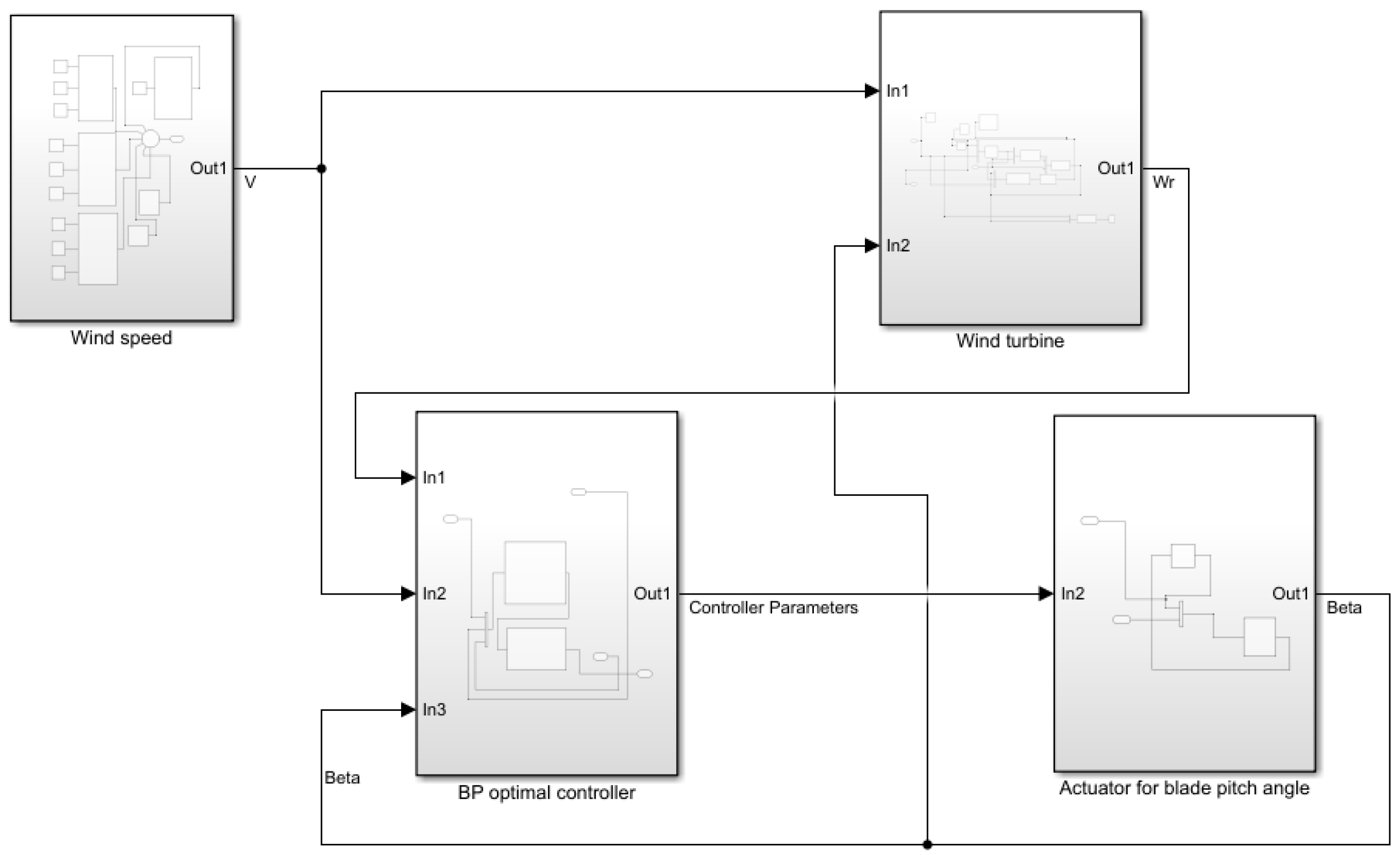
Figure 2 shows the simulation model built in MATLAB/Simulink 2019b. The wind speed module includes the modeling of step wind speed, step wind speed under wind shear effect, real-time wind speed and mixed wind speed. The wind turbine module is modeled according to the Formula (4). The actuator for the blade pitch angle is established based on Formula (6). The BP optimal controller consists of LQR (Linear Quadratic Regulator) controllers and a BP neural network.
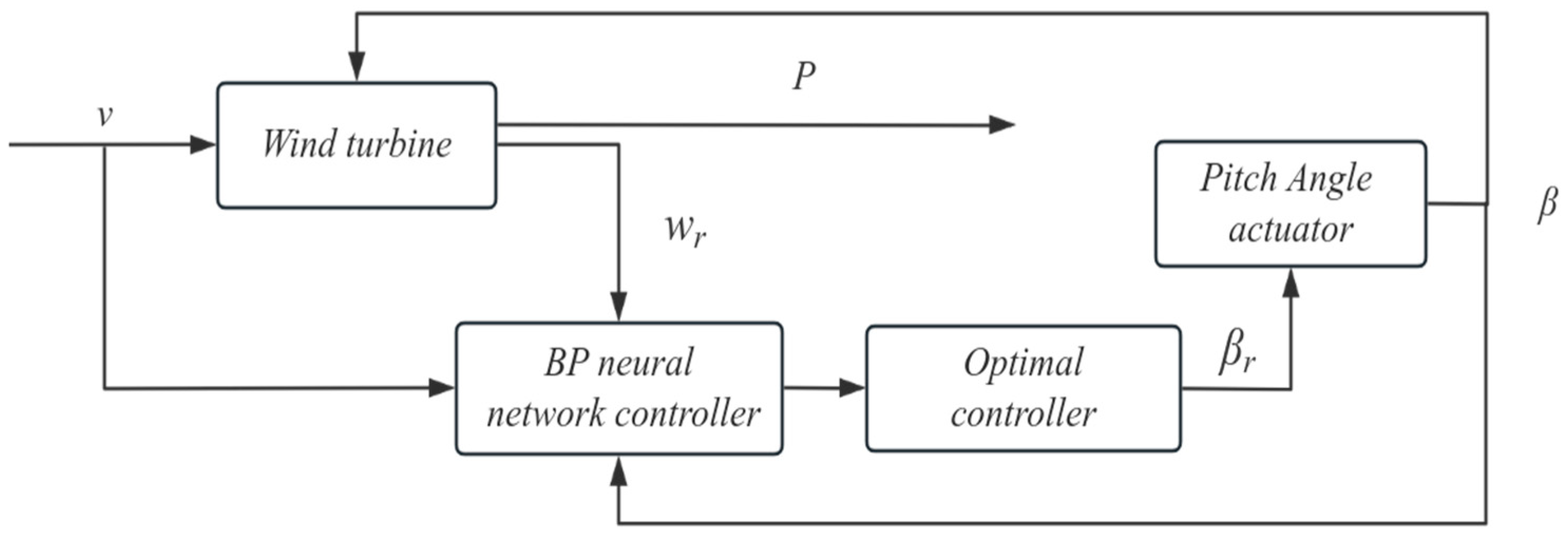
This study primarily investigates the operation of wind turbine generators at wind speeds exceeding the rated wind speed. By using a pitch control mechanism to adjust the pitch angle in real time, the wind turbine can maintain stable operation and constant output power. In the area above the rated wind speed, known as region 3, the pitch control system adjusts the pitch angle β to maintain a stable power output, thereby keeping the generator torque constant. The control idea of the BP optimal controller is shown in Figure 3, where the control input is the wind speed v and the control output is the power P, which is directly related to the rotor speed ωr. The wind speed v, rotor speed ωr and pitch angle β are set as inputs to the neural network. The neural network adjusts the optimal controller in real time to regulate the pitch angle controller βr according to circumstances. The pitch angle actuator adjusts the pitch angle β in real time based on the controller, thereby maintaining a constant system rotor speed and stable output power P. Before constructing a controller for the system, it can be noted from Equation (5) that it is a typical nonlinear uncertain system with non-affine control inputs. Therefore, we first need to linearize the model.

2.2. Linearization of Wind Turbine

For the model, the first-order Taylor expansion of Equation (5) is carried out at different steady-state operating conditions i o = ( x ¯ , u ¯ ) , and the following results are obtained:
d T a e r o = T a e r o ( x , u ) T a e r o ( x , u ) = d T a e r o d ω r | i o d ω r + d T a e r o d β | i o d β = F ω d ω r + F β d β
where symbol d is the deviation of the variable from the steady-state point; x , u ¯ are the state variable and the steady state value of the input variable during steady state operation. Fβ and Fω are, respectively, the coefficients of the corresponding terms of ωr and β after linearization.
The general form is as follows:
( β . ω r . ) = ( A 11 A 12 A 21 A 22 ) ( β ω ) + ( B 11 B 21 ) u
y = ( C 1    C 2 ) ( β ω r )
According to the order of Formula (6), we make ψ 1 = β , ψ 2 = ω r and Formula (11) is obtained.
{ ψ 1 = 1 T β ( β r β ) ψ 2 = 1 J ( T a e r o T g e n T f )
The four elements of matrix A can be calculated by the following formulas: A11 is obtained by calculating the partial derivative of ψ 1 with respect to β, A12 is obtained by calculating the partial derivative of ψ 1 with respect to ωr, A21 is obtained by calculating the partial derivative of ψ 2 with respect to β and A22 is obtained by calculating the partial derivative of ψ 2 with respect to ωr.
A 11 = ψ 1 β ,   A 12 = ψ 1 ω r ,   A 21 = ψ 2 β ,   A 22 = ψ 2 ω r .
Matrix A can be written in the following format:
A = [ ψ 1 β    ψ 1 ω r ψ 2 β    ψ 2 ω r ]

3. Back-Propagation Optimal Controller Design

The paragraph aims to design an optimal controller for a WTGS and construct a neural network to adjust the optimal controller based on real-time input parameters.

3.1. Design of Optimal Controller

LQR is a widely used optimization control method. By designing weight matrices Q and R, the system’s performance index J is minimized, resulting in the optimal control feedback matrix K [32].
Secondary performance indicators may be articulated as follows:
J = 0.5 t 0 t f [ e T Q e + u T R u ] d t + 0.5 e T ( t f ) Q 0 e ( t f )
Firstly, the LQR problem is formulated as a Riccati equation. For the system described previously, the Riccati equation is as follows:
A T P + P A P B R 1 B T + Q = 0
where P is a symmetric positive definite matrix, representing the state feedback matrix. By solving the Riccati equation, P is calculated and the optimal state feedback matrix is obtained:
K = R 1 B T P
According to the minimum principle, the n-dimensional costate vector λ ( t ) is introduced to construct the Hamilton function:
H ( x , u , λ , t ) = 1 2 [ x T Q 1 ( t ) x + u T Q 2 ( t ) u ] d t + λ T [ A ( t ) x ( t ) + B ( t ) u ( t ) ]
u = R 1 ( t ) B T ( t ) P ( t ) x ( t ) = K ( t ) x ( t )
For the above nonlinear system, the equation of state of the system is solved by Taylor expansion. The B, C matrix can be obtained as follows:
B = ( B 11 B 21 ) = ( 1 T β 0 )    C = ( 0    1 )
Because the system is a nonlinear system, the system state equation changes according to the change in wind speed, and the control effect of a single optimal controller is mediocre when solving the constant power problem of the system, and the system cannot achieve steady state operation.
By adjusting the wind speed variable, the state variable of the system under different wind speed is obtained, and the optimal controller of the system under different wind speed is solved according to the optimal control algorithm, so as to ensure that each sub-controller can ensure the stable operation of the system under the corresponding wind speed.
In this experiment, the 12 wind conditions of 11 m/s, 12 m/s, 13 m/s, 14 m/s, 15 m/s, 16 m/s, 17 m/s, 18 m/s, 19 m/s, 20 m/s, 21 m/s and 22 m/s are used to design sub-controllers u1, u2, u3, u4, u5, u6, u7, u8, u9, u10, u11 and u12. Then, the sub-controller is inserted into the system model and its control effect is observed.
Sub-controller data are as follows:
If v 1 = 11 m/s, we obtain u 1 = 4.6 × ω r − 0.079 × β − 23.
If v 2 = 12 m/s, we obtain u 2 = 14.08 × ω r − 0.08 × β − 57.76.
If v 3 = 13 m/s, we obtain u 3 = 16.69 × ω r − 0.11 × β − 75.13.
If v 4 = 14 m/s, we obtain u 4 = 20.22 × ω r − 0.091 × β − 64.015.
If v 5 = 15 m/s, we obtain u 5 = 25.25 × ω r − 0.202 × β − 92.23.
If v 6 = 16 m/s, we obtain u 6 = 32.80 × ω r − 0.37 × β − 118.85.
If v 7 = 17 m/s, we obtain u 7 = 33.83 × ω r − 0.36 × β − 120.38.
If v 8 = 18 m/s, we obtain u 8 = 38.2 × ω r − 0.41 × β − 136.56.
If v 9 = 19 m/s, we obtain u 9 = 43.09 × ω r − 0.57 × β − 150.8.
If v 10 = 20 m/s, we obtain u 10 = 46.69 × ω r − 0.56 × β − 161.33.
If v 11 = 21 m/s, we obtain u 11 = 54.52 × ω r − 0.86 × β − 188.28.
If v 12 = 22 m/s, we obtain u 12 = 57.42 × ω r − 0.91 × β − 195.53.

3.2. Back-Propagation Optimal Controller Design

A BP neural network is a multi-layer feed-forward neural network trained using the error back-propagation algorithm, where the weights of neurons are continuously adjusted through gradient descent to minimize approximation errors. In comparison to the RBF neural network, it has a simpler network structure with fewer hidden-layer neurons and lower computational requirements. Assuming that the number of nodes in the input layer is denoted as n, the number of nodes in the hidden layer denoted as l needs to be iteratively determined to achieve optimal values for minimizing approximation errors, while m represents the number of nodes in the output layer. The weight from the input layer to hidden layer is represented by υ i j , and from the hidden layer to output layer by μ j k . Additionally, bias from the input layer to hidden layers is denoted as a, and bias from the hidden layers to output layers as b. The learning rate is represented by η and the sigmoid function serves as an activation function g(x):
g ( x ) = 1 1 + e x
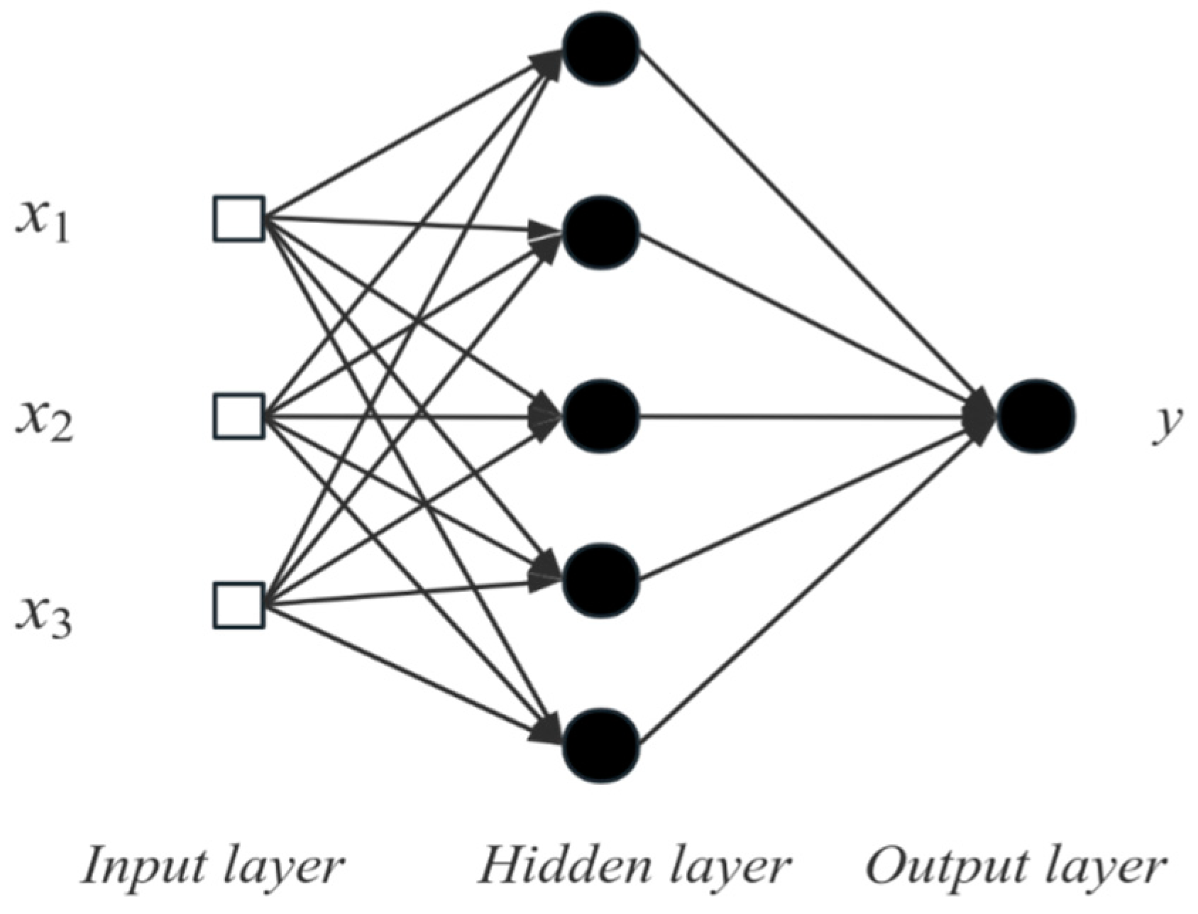
The optimal control parameters in this paper are obtained by the adaptive prediction model of a BP artificial neural network. The network structure of the BP neural network is shown in Figure 4 below.
The design of this system includes an input layer with three units, an output layer with one unit, and a hidden layer with five units. The training process involves running the system for 2000 iterations, aiming to achieve an error range of 0.000006 and utilizing a learning rate of 0.01. The inputs consist of parameters such as wind speed, rotor speed, and blade pitch angle, while the outputs represent optimal controller control parameters.
{ x 1 = ω r x 2 = β x 3 = v
The data from the input layer are xn, the parameters from the input layer to the hidden layer are υ ij and a, the parameters from the hidden layer to the output layer are μ jk and b and the activation functions are g1 and g2. Then, the model is set as follows:
Input layer to hidden layer:
n e t 1 = υ i j T x + a , h = g 1 ( n e t 1 )
Hidden layer to output layer:
n e t 2 = μ j k T h + b , y ^ = g 2 ( n e t 2 )
Model:
y ^ = g 2 ( n e t 2 ) = g 2 ( μ j k T g 1 ( υ i j T x + a ) + b )
Among them:
x = ( x 1 x 2 x 3 ) ,   υ i j = ( υ 11 υ 15 υ 21 υ 25 υ 31 υ 35 ) ,   a = ( a 1 a 2 a 3 a 4 a 5 ) ,   n e t 1 = ( n e t 11 n e t 12 n e t 13 n e t 14 n e t 15 ) ,   h = ( h 1 h 2 h 3 h 4 h 5 ) , μ j k = ( μ 11 μ 21 μ 31 μ 41 μ 51 ) ,
b = ( b 1 ) ,   n e t 2 = ( n e t 2 ) ,   y ^ = ( y ^ ) ,   y = ( y )
Implementation steps:
(1) The weights and bias terms in the initial network are denoted as follows: υ i j ( 0 ) ,   μ j k ( 0 ) ,   a ( 0 ) ,   b ( 0 ) .
The activation forward propagation is as follows:
{ n e t 11 = υ 11 ω r + υ 21 β + υ 31 v + a 1 n e t 12 = υ 12 ω r + υ 22 β + υ 32 v + a 1 n e t 13 = υ 13 ω r + υ 23 β + υ 33 v + a 3 n e t 14 = υ 14 ω r + υ 24 β + υ 34 v + a 4 n e t 15 = υ 15 ω r + υ 25 β + υ 35 v + a 5
According to the excitation function,
o u t h 1 = 1 1 + e n e t h 1 ,   o u t h 2 = 1 1 + e n e t h 2 ,   o u t h 3 = 1 1 + e n e t h 3 , o u t h 4 = 1 1 + e n e t h 4 ,   o u t h 5 = 1 1 + e n e t h 5
n e t 2 = μ 11 o u t h 1 + μ 21 o u t h 2 + μ 31 o u t h 3 + μ 41 o u t h 4 + μ 51 o u t h 5 + b 1
y ^ = 1 1 + e n e t 2 = 1 1 + e ( μ 11 o u t h 1 + μ 21 o u t h 2 + μ 31 o u t h 3 + μ 41 o u t h 4 + μ 51 o u t h 5 + b 1 )
(2) The expected value of each layer output and loss function can then be obtained: E θ = ( y y ^ ) 2 .
(3) Based on the loss function, the error term for both the output unit and hidden unit can be computed. Specifically, the gradient value or partial derivative of the loss function can be calculated with respect to the output unit as an indicator of its error. By applying the chain rule, this can be expressed as follows:
( k ) μ = E μ = n e t 2 μ y ^ n e t 2 E y ^
( k ) b = E b = n e t 2 b y ^ n e t 2 E y ^
The error term of hidden units, denoted as the gradient value or partial derivative of the loss function with respect to hidden units, can be derived using the chain rule:
( k ) υ = E υ = n e t 1 υ h n e t 1 n e t 2 h y ^ n e t 2 E y ^
( k ) a = E a = n e t 1 a h n e t 1 n e t 2 h y ^ n e t 2 E y ^
(4) The weights and biases in the neural network are updated.
Output cell parameter update:
μ k = μ ( k 1 ) η ( k ) μ = μ ( k 1 ) η E μ ,   b k = b k 1 η E b
Hidden cell parameter update:
υ k = υ ( k 1 ) η ( k ) υ = υ ( k 1 ) η E υ ,   a k = a k 1 η E a
Steps 2–4 are repeated until the loss function is less than the pre-given threshold or the number of iterations is exhausted. The output parameter at this time is the best parameter at present.
In the previous section, different optimal controllers were selected to meet the control requirements for corresponding wind speed conditions. The controller gains and the system’s rotor speed and pitch angle data at each wind speed condition were collected in MATLAB 2019b. To avoid overestimating high-amplitude data, it is necessary to normalize the data before training. The minimum–maximum normalization method was used to constrain the data within [0,1], maintaining the zero-mean characteristic of structural vibration, thus improving the performance and stability of the machine learning algorithms.
The learning rate of a neural network is an important hyper-parameter that controls the size of each update to the model parameters during the training process. Specifically, it determines the step size along the gradient direction in gradient descent. In this study, after multiple rounds of training, the learning rate gradually decreased, and eventually a learning rate of 0.01 was chosen.
The term “epochs” in neural network training refers to the number of complete traversals of the entire training dataset. Each complete traversal of the training dataset is called an epoch. During each epoch, the neural network performs one forward pass and one backward pass for each training sample, and updates the model parameters based on the calculated error. The model performance is evaluated during training using a validation set, and by monitoring changes in validation error, the optimal stopping point for training is determined. In this case, 2000 epochs are chosen as the number of training iterations.
The dataset collected through MATLAB 2019b will be used as a training set for network learning and training and gradient descent will be employed for neural network learning and training while establishing mapping between input vectors and output quantities. A network model will be built in MATLAB/Simulink 2019b, where real-time rotor speed, pitch angle and wind speed are applied to train the network to obtain gains.
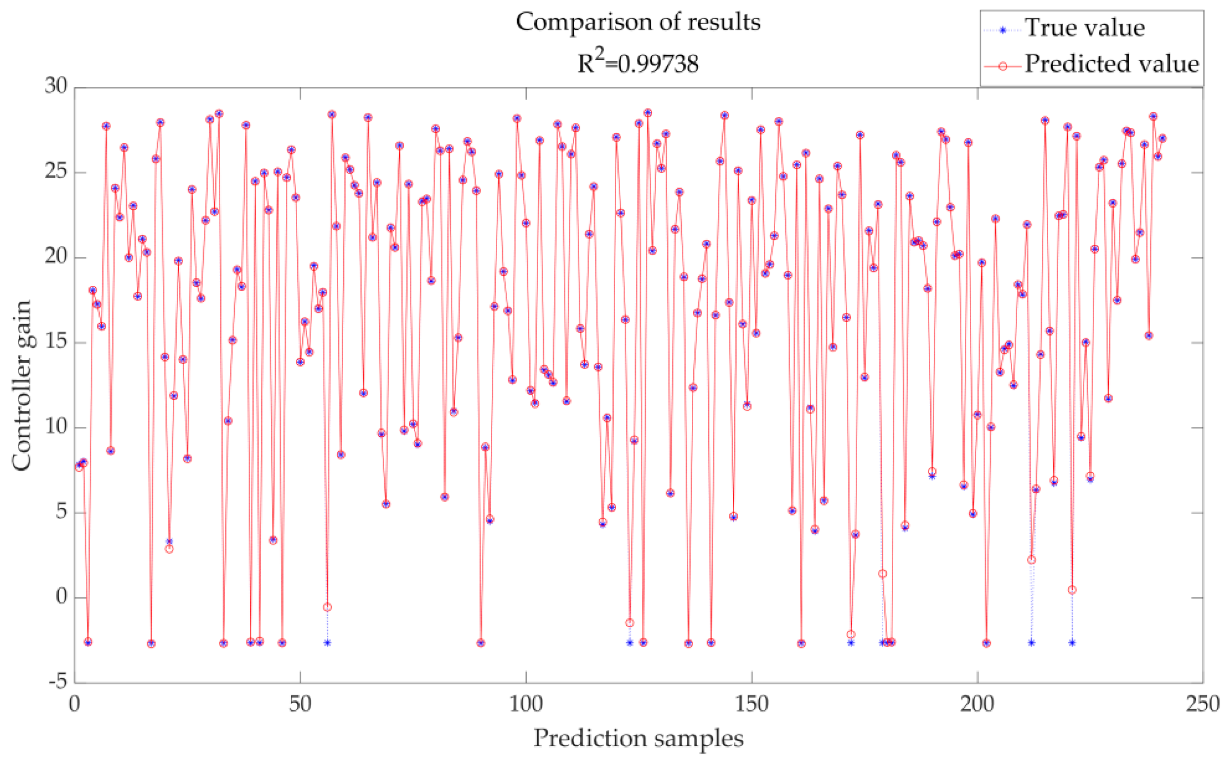
For this wind turbine model, basic system parameters are imported into the system to obtain corresponding rotor speed and pitch angle parameters; continuous data collection yields 200 sets of trained data including rotor speeds under corresponding wind speeds as well as pitch angles and optimal controller parameters for BP neural network training purposes. The trained data are shown in Figure 5 below.
R2 represents the proportion of variance that can be explained by the model and is commonly employed for comparing the performance of different models. In general, the R2 determination coefficient ranges from 0 to 1. A value of 1 indicates perfect prediction by the model.
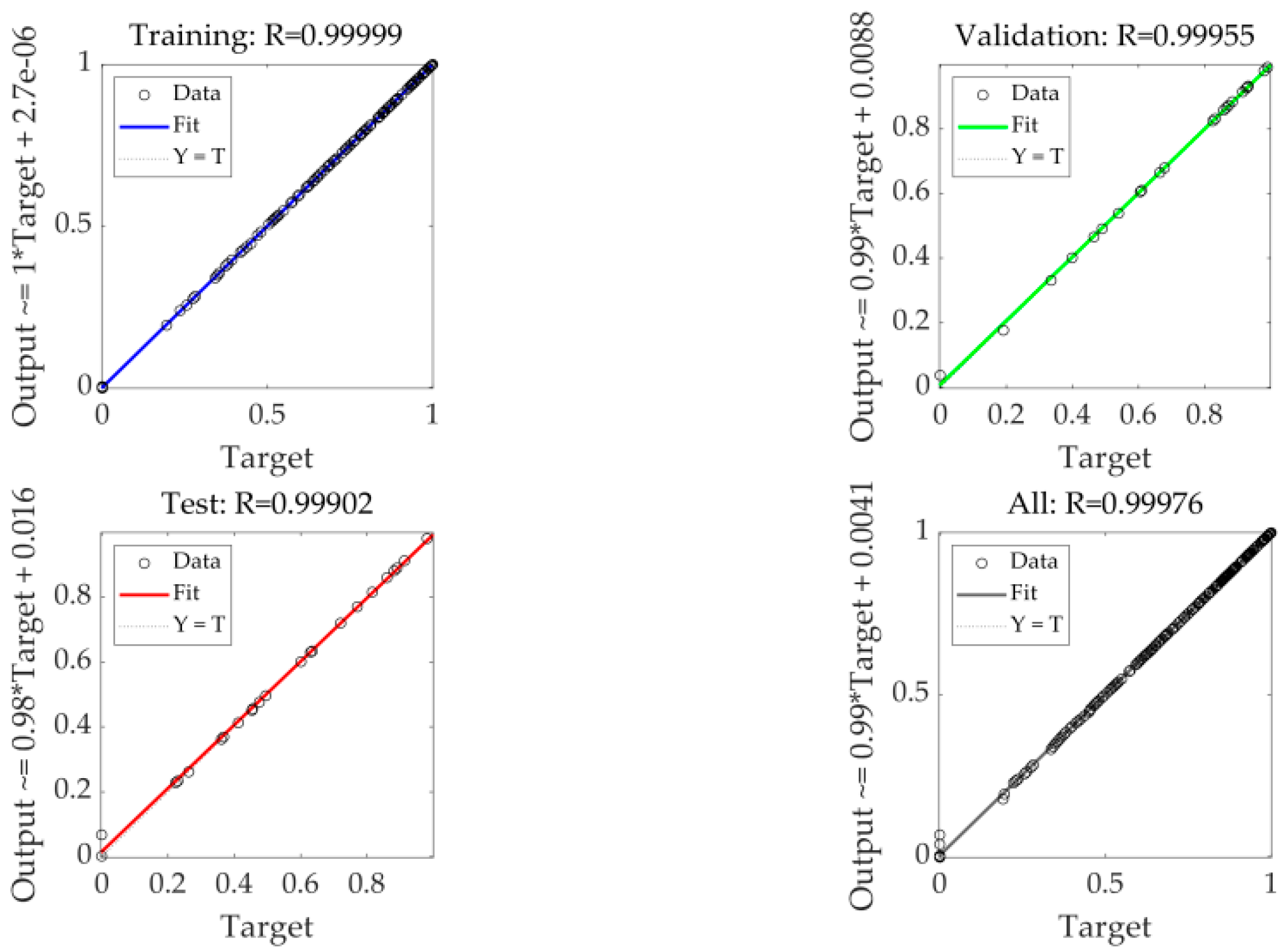
Figure 6 shows that the performance of the network is measured by mean square error, and it can be observed that the more epochs there are, the better the performance. Figure 7 measures the degree of fitting of the corresponding data of the neural network by drawing the regression line for the solution objects in the graph; the R-value in any one case is 0.95+, so it is clear that this fit is reasonable.
When applying a BP neural network to adjust the gain of the optimal controller, the small size of the training dataset or long training time of the network may lead to low computational efficiency. In practical situations, this may result in erroneous operation of the controller. To address this issue, future experiments may focus on improving the network structure or combining optimization algorithms to enhance the computational efficiency of the network.
The trained BP neural network is inserted into the system, and the optimal controller parameters are changed in real time by inputting wind speed, rotor speed and pitch angle, so as to complete the adjustment of pitch angle and make the wind turbine run in a steady state.

4. System Simulation and Result Analysis

In this chapter, modeling and simulations will be conducted in MATLAB 2019b, and the experimental parameters are as follows: the radius of the wind wheel is 21.65 m, the air density is 1.25 kg/m3, the rated rotor speed of the wind turbine is 4.35 rad/s, the rated power of the generator is 0.6 MW, and the total moment of inertia of the wind turbine and the generator is 322,000. The control effects of the BP optimal controller and three other controllers will be compared under four different wind speed scenarios and the respective advantages and disadvantages will be analyzed. Wind speed scenarios are shown in Table 1.
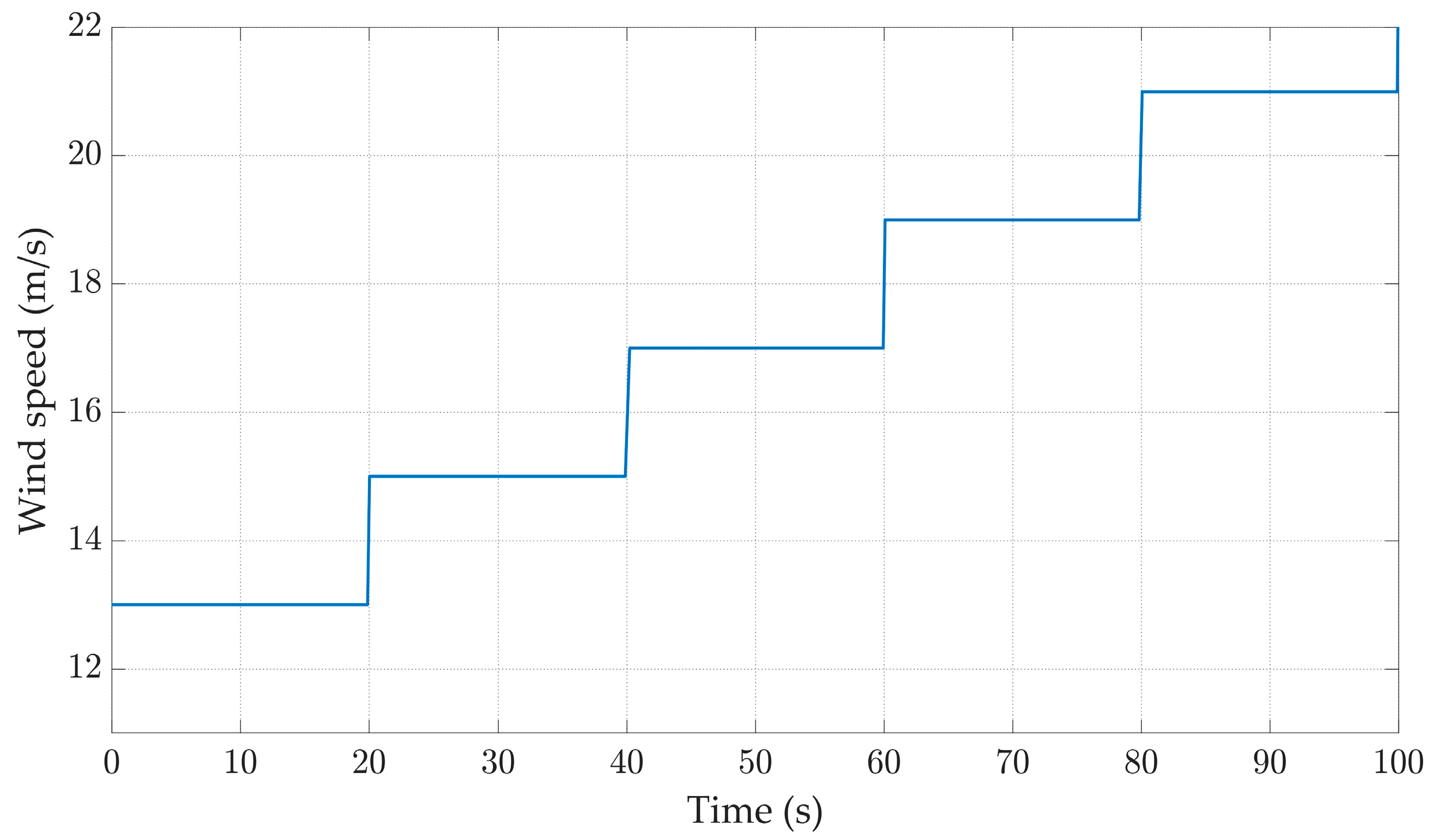
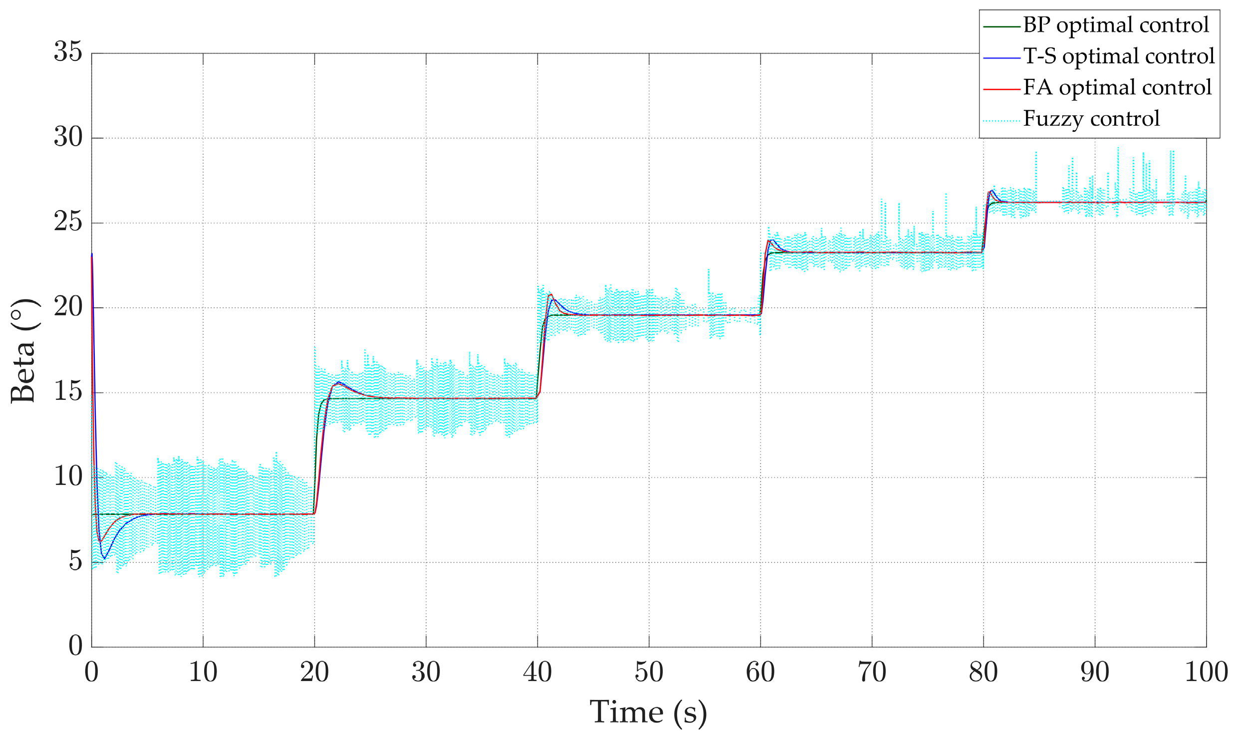
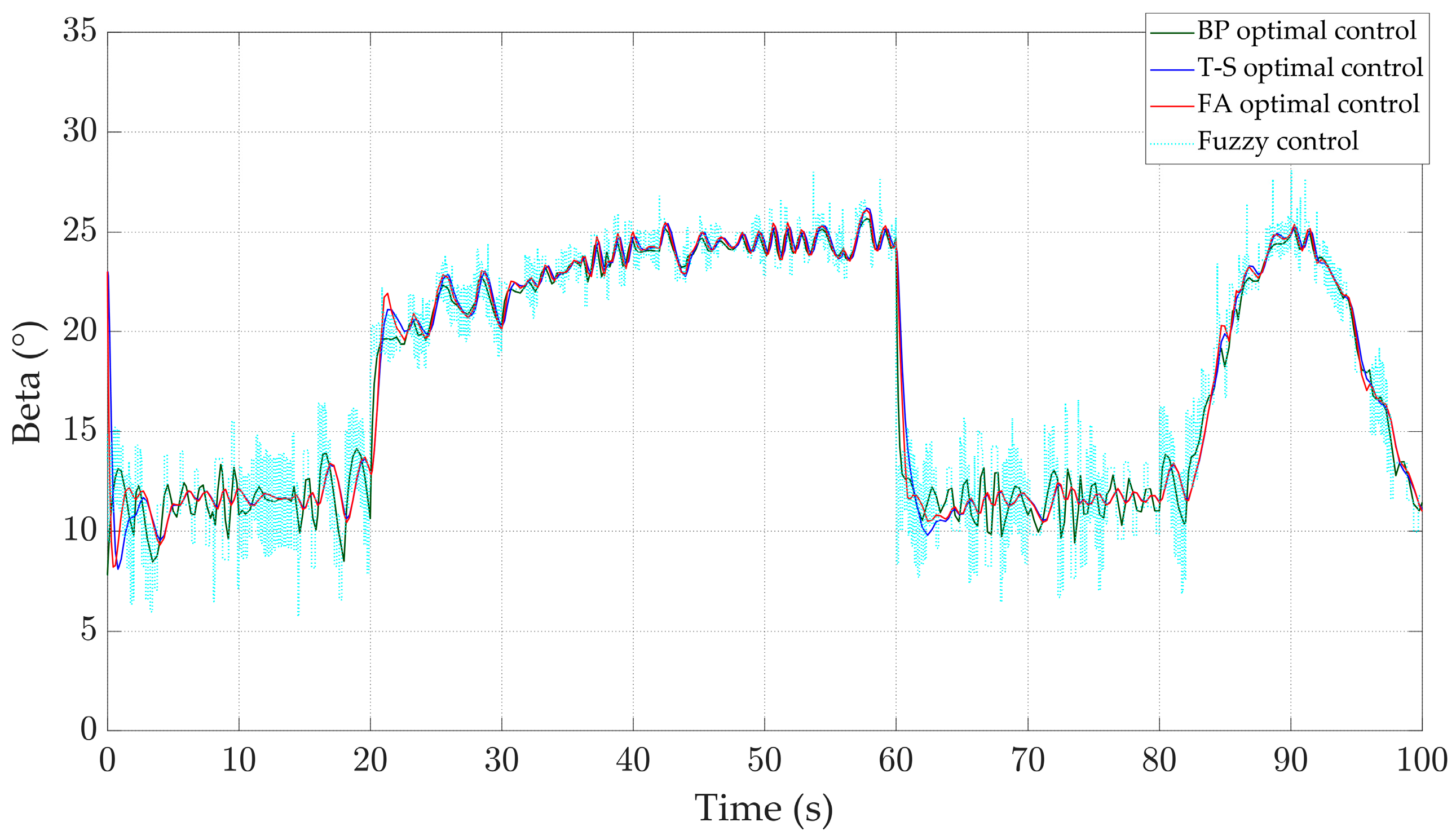
To evaluate the controller’s ability under step wind, a signal with a step of 2 m/s and a range of 13 m/s to 21 m/s is input into MATLAB/Simulink 2019b, as shown in Figure 8. As depicted in Figure 9, when adjusting the pitch angle, the BP optimal controller exhibits a better response speed and overshoot performance. At 40 s, there is almost no overshoot when the pitch angle is adjusted by the BP optimal controller. The peak pitch angles for the T-S optimal controller and FA optimal controller are, respectively, 0.87° and 1.24° higher than that of the BP optimal controller, with response times exceeding 3 s, significantly longer than that of the BP optimal controller. Meanwhile, the fuzzy controller shows mediocre control effects with continuous oscillations in propeller pitch angle waveform.
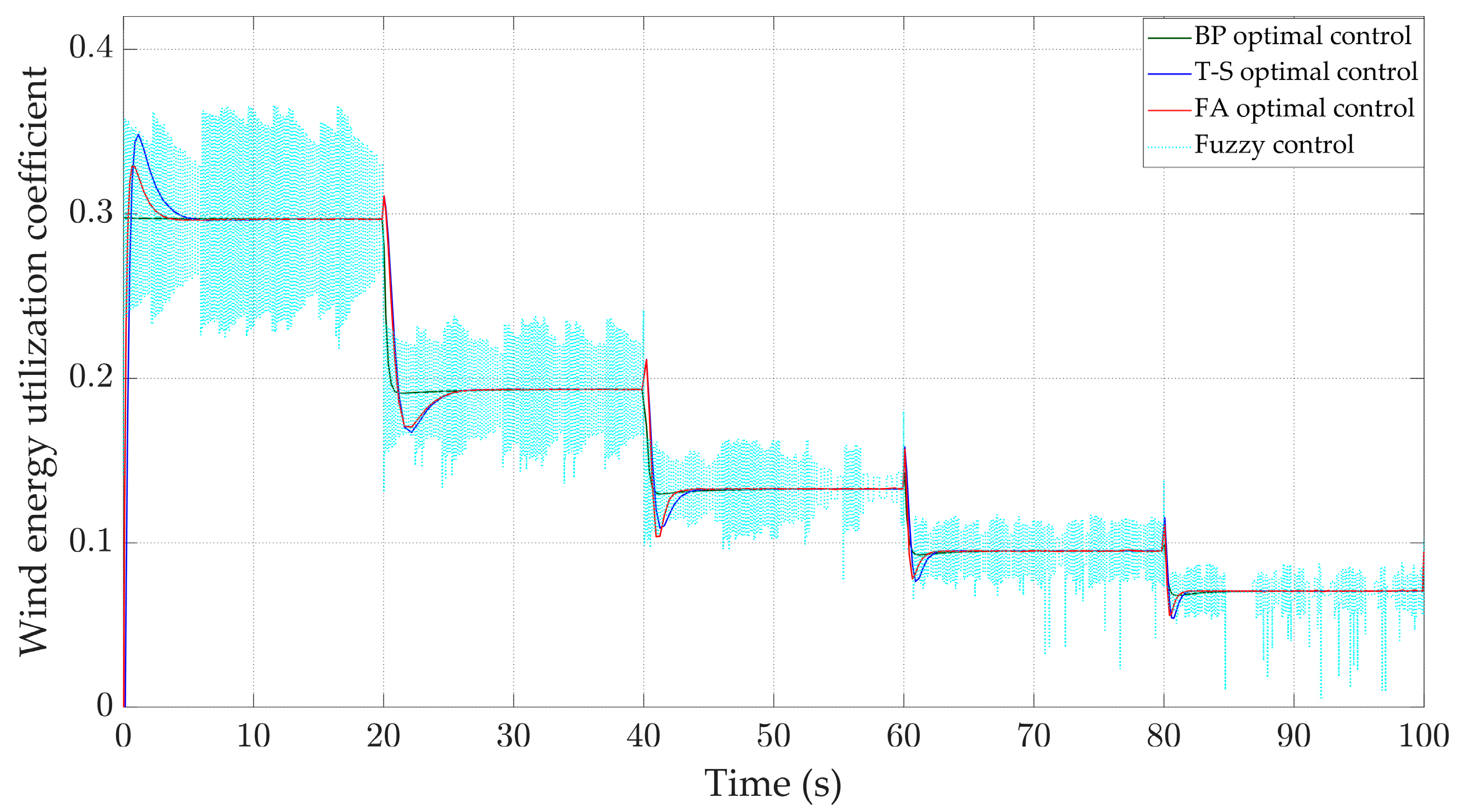
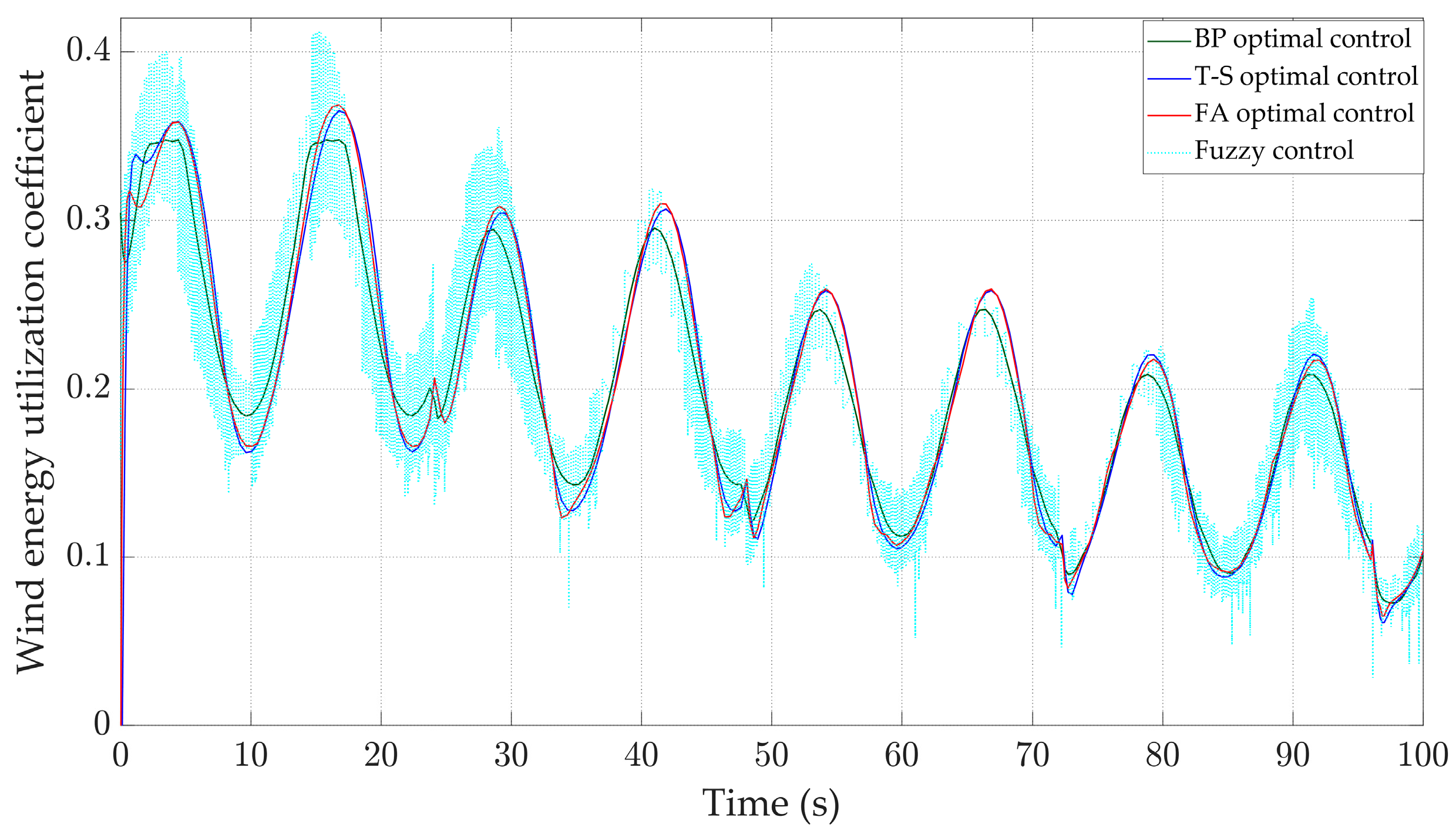
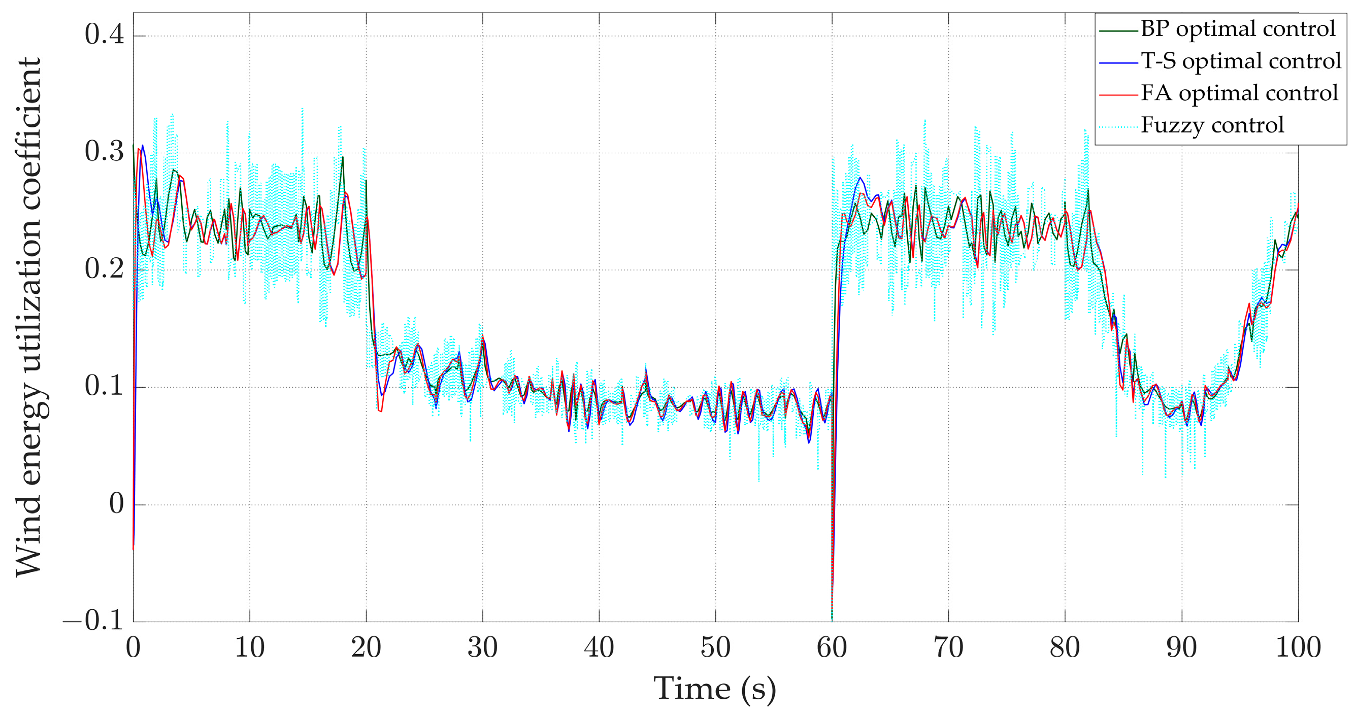
The wind energy utilization coefficients of the four controllers are shown in Figure 10. The BP optimal controller exhibits almost no overshoot at the 40th second, with a response time of only 1 s. In contrast, both the T-S optimal controller and FA optimal controller have response times close to 2 s and show some degree of overshoot. The fuzzy controller’s wind energy utilization coefficient oscillates throughout and cannot maintain a constant value. It is evident that compared to the T-S optimal controller, FA optimal controller and fuzzy controller, the control stability of the BP optimal controller is far superior.
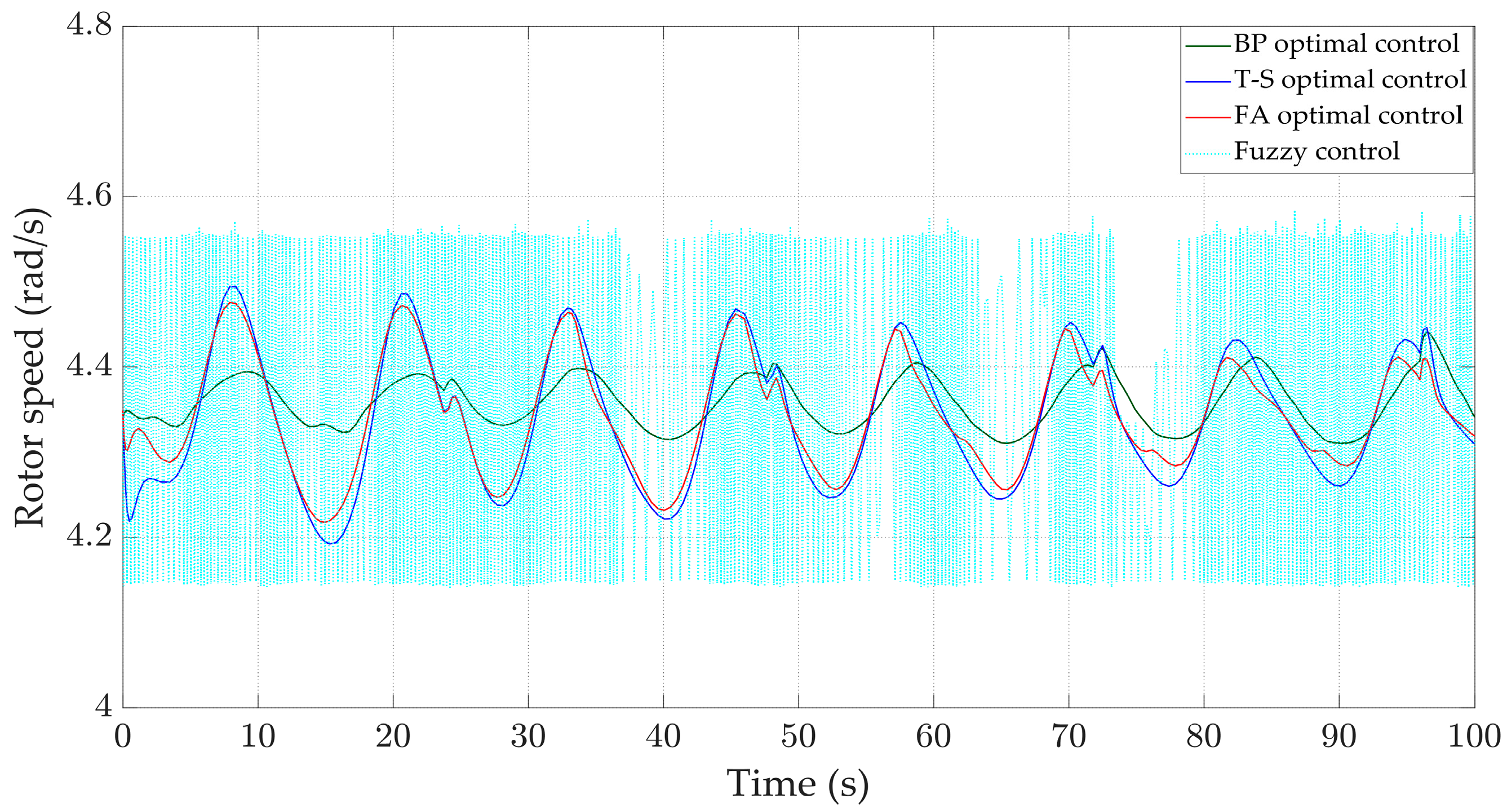
Figure 11 shows the curves of rotor speed controlled by the four controllers. At 20 s, the peak speed under the BP optimal controller is 4.39 rad/s with a response time of approximately 12 s. Meanwhile, under the T-S optimal controller, the peak speed is 4.5 rad/s with a response time of around 6 s. Under the FA optimal controller, the peak speed is 4.48 rad/s with a response time of around 7 s. The fuzzy controller’s speed fluctuates between 4.15 rad/s and 4.55 rad/s, unable to maintain constant. From the data above, it can be seen that the peak speed under the BP optimal controller is 1% higher than the rated value, while the T-S optimal controller is 3.44% higher, the FA optimal controller is 2.98% higher and the fuzzy controller is 4.59% higher. At the same time, the mean and standard deviation of the rotor speed under the control of the BP optimal controller are 4.359 rad/s and 0.015 rad/s; for the T-S optimal controller, they are 4.355 rad/s and 0.0347 rad/s; for the FA optimal controller, they are 4.357 rad/s and 0.025 rad/s; and for the fuzzy controller, they are 4.346 rad/s and 0.181 rad/s. It is evident that the BP optimal controller has significant advantages in terms of accuracy compared to the T-S optimal controller, FA optimal controller, and fuzzy controller, with a smaller overshoot as well.
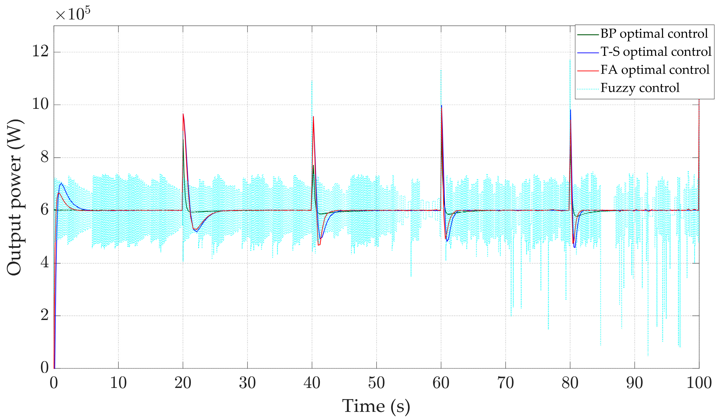
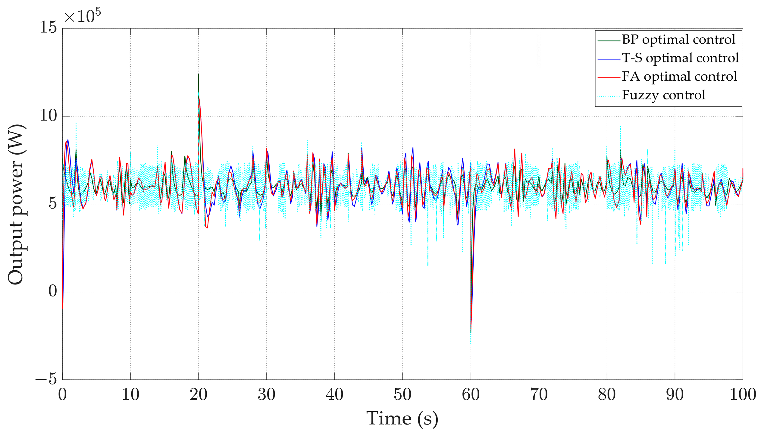
The output power data are shown in Figure 12 and Table 2. At 40 s, the peak power under the BP optimal controller is 0.76 MW, with a response time of around 1 s. In contrast, the peak power under the T-S optimal controller and FA optimal controller is 0.96 MW for both, with a response time of around 2 s, which are higher than those of the BP optimal controller by 0.20 MW and 1 s, respectively. The fuzzy controller achieves a peak power reaching 1.11 MW and a minimum power of 0.44 MW, showing much less effective control compared to the BP optimal controller. Based on the graph, it can be observed that the BP optimal controller exceeds the rated power by 26.67%, while both the T-S and FA controllers exceed the rated power by 60%. In contrast, the fuzzy controller’s maximum and minimum powers are 45% higher and 31% lower than the rated power, respectively. Furthermore, compared to the T-S and FA optimal controllers, the BP optimal controller reduces the response time by one second. Based on these data, it can be inferred that the BP optimal controller demonstrates better control performance in terms of overshoot, response time and overall effectiveness when compared to the T-S and FA optimal controllers and the fuzzy controller. Additionally, there were no oscillations observed with the BP optimal controller after 80 s; its control waveform remained stable during this period.
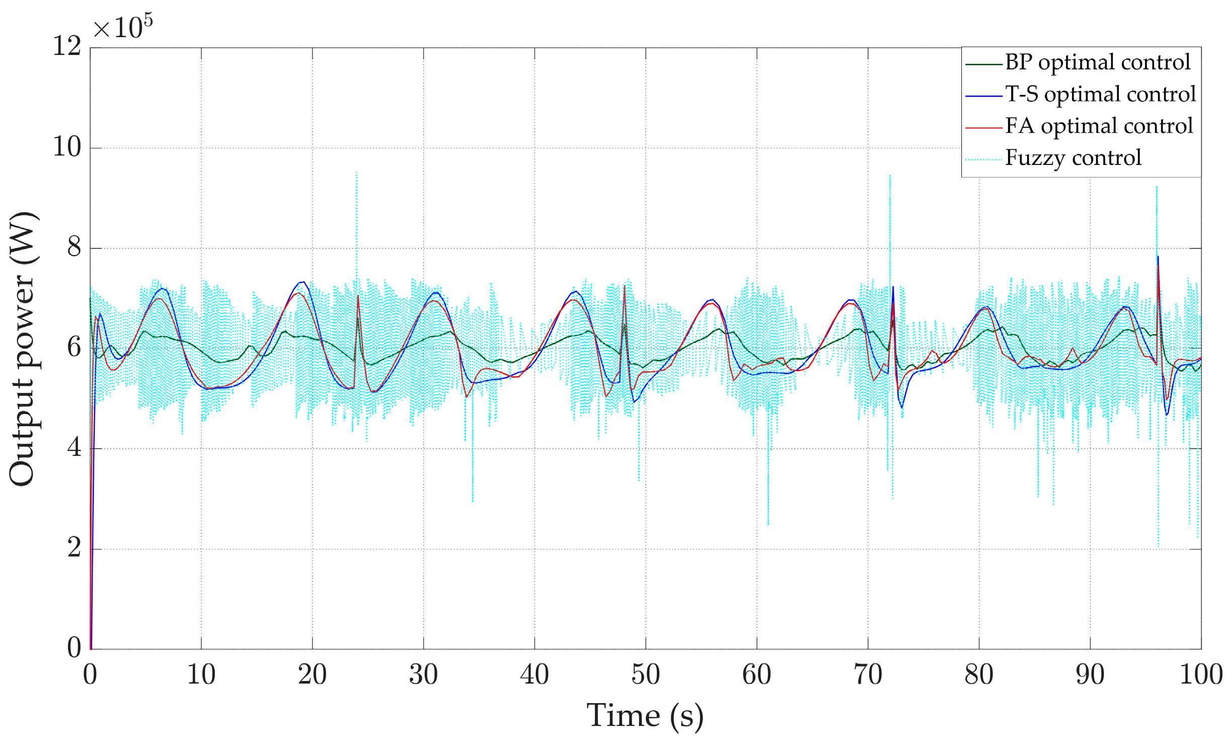
The wind shear effect refers to the phenomenon where wind speed varies with height. The wind shear effect can affect the power output and stability of wind turbines. As shown in Figure 13, adding wind shear to a step wind speed of 13–21 m/s results in a continuous upward sine signal of wind speed with height. The response waveform is shown in Figure 14, Figure 15, Figure 16 and Figure 17. It can be observed that under the action of the BP optimal controller, the range of rotor speed variation is the smallest, between 4.3 and 4.45 rad/s, and tends to stabilize after 40 s, with only a fluctuation of 0.15 rad/s. At the same time, the standard deviation of rotor speed is 0.032 rad/s under BP optimal control, which is 0.045 rad/s less than the T-S optimal controller, 0.031 rad/s less than the FA controller and 0.15 rad/s less than the fuzzy controller. According to Figure 17 and Table 3, the output power of the BP optimal controller is closer to 0.6 MW and the maximum power is only 0.63 MW, resulting in more stable power generation efficiency. It can be seen that when facing wind shear effects, BP optimal control is more stable and robust than the other three controllers.
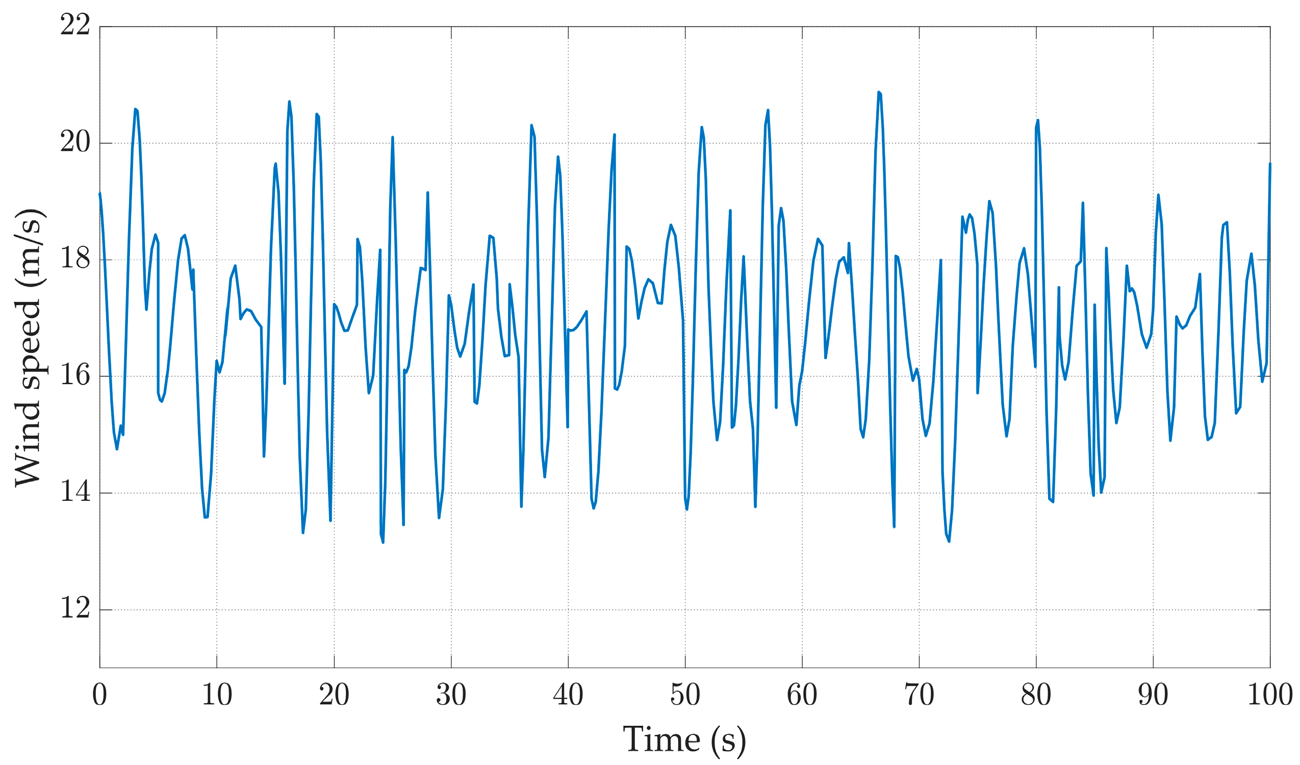
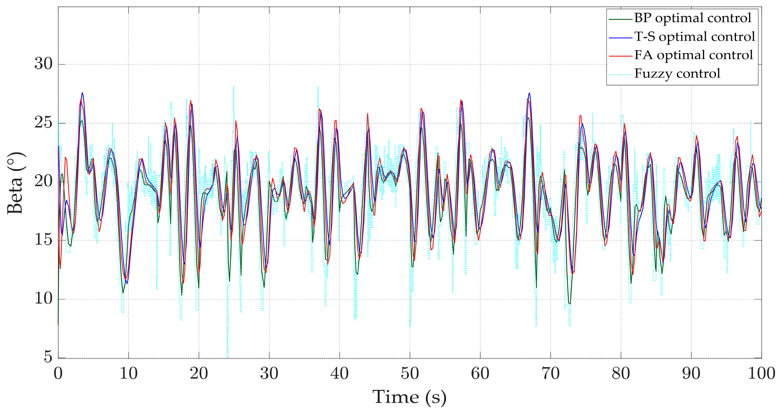
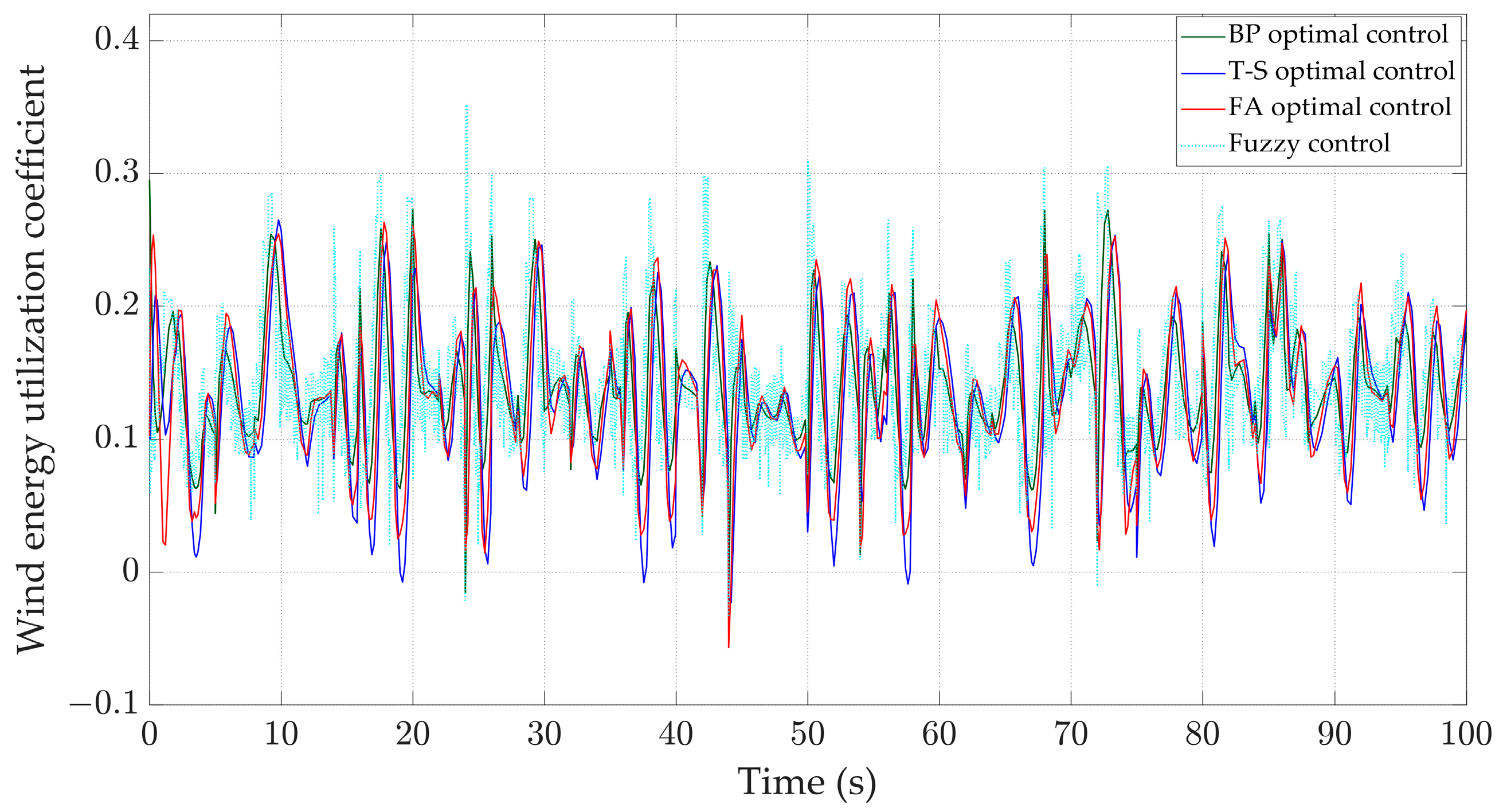
According to reference [33] and the real-time measurement of wind speed in Yancheng City on very windy days, Figure 18 is drawn. When the input of the wind turbine is real-time wind speed, the variation curves of various physical quantities of the WTGS are shown in Figure 19, Figure 20, Figure 21 and Figure 22. Compared to the other three controllers, the BP optimal controller can better stabilize the rotor speed around 4.35 rad/s, and the oscillation range is between 4.31 and4.58 rad/s, which is smaller than that of the other controllers; at the same time, the rotor speed under the control of the BP optimal controller has the smallest standard deviation of 0.041 rad/s. According to Table 4, it can be concluded that the maximum speed and minimum speed under the BP optimal controller are 4.52 rad/s and 4.30 rad/s, which are closer to the stable values than those of the other controllers. According to Figure 22, it can be seen that its output power is also more stable, fluctuating around 0.6 MW with a smaller range of fluctuation. At the same time, the pitch angle changes rapidly, the response speed is fast, which shows better stability.
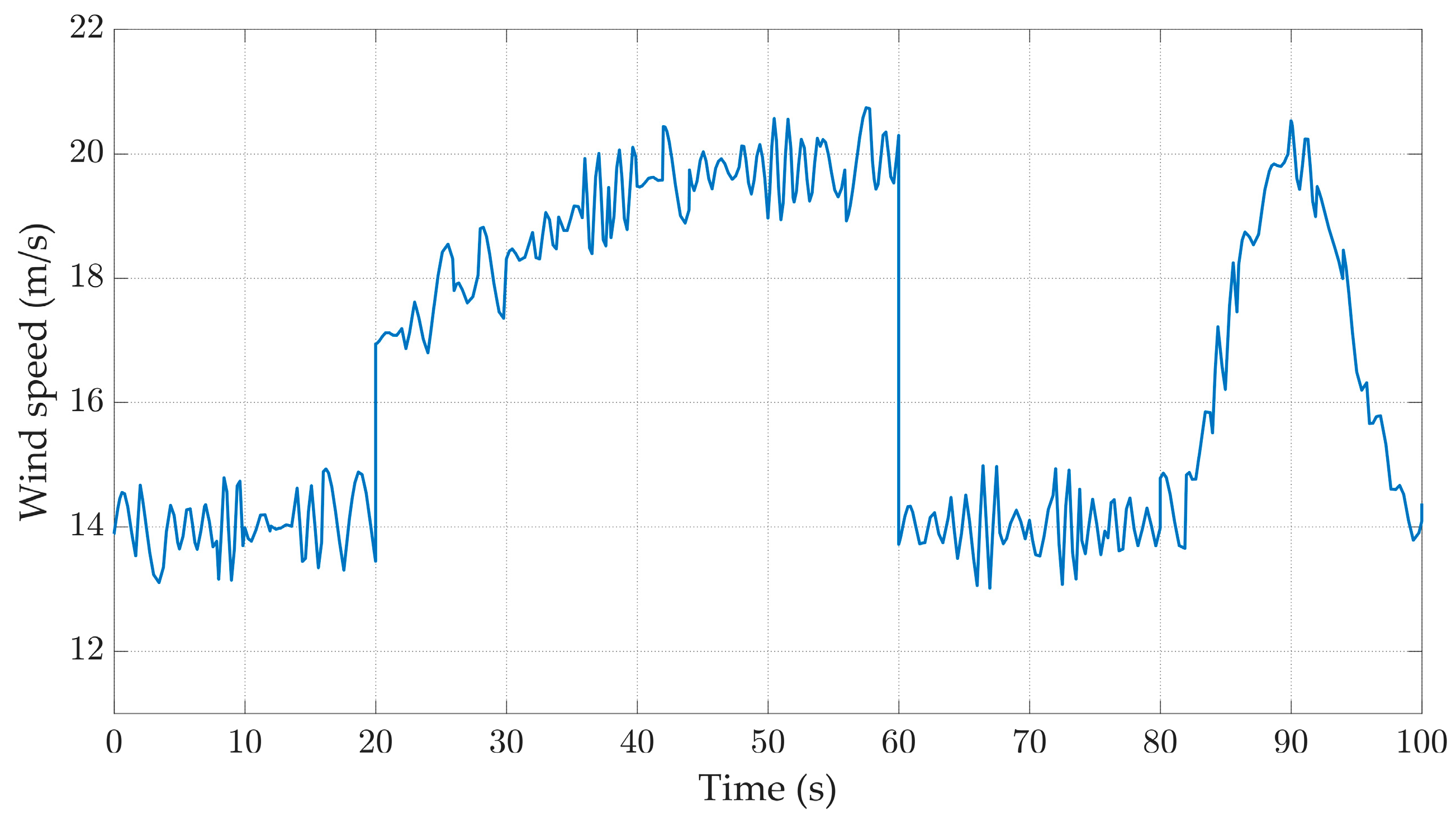
When the input to the system is mixed wind, the response curves of various physical quantities are shown in Figure 23, Figure 24, Figure 25, Figure 26 and Figure 27. Compared with the other three controllers, the BP optimal controller can more stably control the pitch angle and wind energy utilization coefficient. According to the data in Table 5 and Figure 26, compared with other controllers, the BP optimal controller can better stabilize the rotor speed around 4.35 rad/s, and has the smallest oscillation range and the smallest standard deviation of 0.028 rad/s. As shown in Figure 27, the output power curve of the BP optimal controller is more stable, and the frequency of exceeding 0.8 MW and being below 0.5 MW is significantly lower than the other three controllers. Therefore, the control effect of the BP optimal controller is more stable.

5. Conclusions and Prospect

This paper proposes a variable pitch control strategy based on optimal theory and a BP neural network. To ensure the steady-state operation of the WTGS, the controller aims to maintain the rotor speed and output power constant when the wind speed exceeds the rated value. By training the neural network to dynamically adjust the parameters of the optimal controller in real time, system stability is ensured, thus preventing malfunctions.
This paragraph will compare the performance of the controllers under different wind speeds. Under step wind speed, the rotor speed of the optimal BP controller has the smallest maximum of 4.4 rad/s, which is 0.11 rad/s smaller than that of the T-S optimal controller, 0.09 rad/s smaller than that of the FA optimal controller and 0.22 rad/s smaller than that of the fuzzy controller. At the same time, the optimal BP controller has almost no overshoot, indicating more stable control. Considering the effect of wind shear, the rotor speed fluctuation of the optimal BP controller is minimal, ranging from 4.3 rad/s to 4.45 rad/s with an oscillation range of 0.15 rad/s. This oscillation range is 38% smaller than that of the T-S optimal controller, 25% smaller than that of the FA optimal controller and significantly 70% smaller than that of the fuzzy controller. Under the other two wind speed conditions, the fluctuation range of the rotor speed of the BP optimal controller is always the smallest, and it can best stabilize near 4.35 rad/s. In conclusion, it can be inferred that compared to other controllers, the BP optimal controller has better control effects. It can better ensure that the system operates under steady-state conditions, maintains the rotor speed constant, and has stronger anti-interference ability when facing different wind speeds.
Future research prospects: (1) a BP neural network is prone to overfitting and significant errors when facing rapid changes in wind speed. Therefore, in the future, other optimization algorithms can be combined with a BP neural network to increase the total amount of data for improvement. (2) This study did not consider the control objective of wind speed below the rated value. In the future, we will conduct research on this operating condition to achieve the control of the entire wind speed range. (3) Due to the fluctuation and instability of wind energy, many wind farms are currently equipped with energy storage stations to regulate it. So, in the future, the research focus can be shifted to energy storage devices.

Author Contributions

S.Q. carried out the majority of the work in this paper. Z.C. participated in the experiments. All authors have taken part in the data analysis and interpretation. All authors have read and agreed to the published version of the manuscript.

Funding

I would like to thank the School of Electrical Engineering, Yancheng Institute of Technology, and the Department of Electrical and Electronic Engineering, Faculty of Engineering, Universiti Malaysia Sarawak for the funding, the funding number is UNI/F02/GRADUATES/85400/2022.

Data Availability Statement

The raw data supporting the conclusions of this article will be made available by the authors on request.

Acknowledgments

Throughout the writing of this dissertation, I have received a great deal of support and assistance. I would particularly like to acknowledge my teammate/group mate/team members, Zhipeng Cao, Sze Song Ngu, Lee Chin Kho, Hui Cai and Feng Wang, for their wonderful collaboration and patient support. Finally, I am really grateful to all those who have devoted much time to reading this thesis and have given me much advice, which will benefit me in my later study.

Conflicts of Interest

The authors declare no conflicts of interest.

References

  1. Strong 2023 Offshore Wind Growth as Industry Sets Course for Record-Breaking Decade. Available online: https://gwec.net/strong-2023-offshore-wind-growth-as-industry-sets-course-for-record-breaking-decade/ (accessed on 17 June 2024).
  2. Zhang, M.; Cong, N.; Song, Y.; Xia, Q. Cost analysis of onshore wind power in China based on learning curve. Energy 2024, 291, 130459. [Google Scholar] [CrossRef]
  3. Liu, X. Research on pitch control and low voltage crossing technology of doubly-fed wind turbine. Appl. Energy Technol. 2023, 6, 39–43. [Google Scholar]
  4. Lu, S.-X.; Shi, H. Technical analysis of pitch angle control for wind turbine. Integr. Circuit Appl. 2023, 40, 70–72. [Google Scholar]
  5. Yang, B.; Yang, L. Research on Robust Control of Variable Speed and Variable Pitch Permanent Magnet Synchronous Wind Turbine; Kunming University of Science and Technology: Kunming, China, 2022. [Google Scholar]
  6. Ren, H.; Zhang, H.; Zhou, H.; Zhang, P.; Lei, X.; Deng, G.; Hou, B. A Novel Constant Output Powers Compound Control Strategy for Variable-speed Variable-Pitch Wind Turbines. IEEE Access 2018, 6, 17050–17059. [Google Scholar] [CrossRef]
  7. Zhang, K.; Lu, W.; Xiong, L.; Wang, M.; Ding, Y. Maximum Power Control of wind Power System based on improved active disturbance rejection. China Electr. Eng. 2022, 12, 7–13+41. [Google Scholar]
  8. Qin, S.; Hu, G.; Gu, C.; Li, D. Constant Power Nonlinear H∞ Robust Control of Wind Power System. Control Theory Appl. 2012, 29, 617–622. [Google Scholar]
  9. Ren, B.; Jia, Y.; Li, Q.; Wang, D.; Tang, W.; Zhang, S. Robust Wind Power Ramp Control Strategy Considering Wind Power Uncertainty. Electronics 2024, 13, 211. [Google Scholar] [CrossRef]
  10. Lasheen, A.; Elnaggar, M.; Yassin, H. Adaptive control design and implementation for collective pitch in wind energy conversion systems. ISA Trans. 2020, 102, 251–263. [Google Scholar] [CrossRef]
  11. Yang, Q.M.; Jiao, X.G.; Sun, Y.X. L1 adaptive pitch angle controller of wind energy conversion systems. ISA Trans. 2020, 103, 28–36. [Google Scholar] [CrossRef] [PubMed]
  12. Phung, B.N.; Wu, Y.-K.; Pham, M.-H. Novel Fuzzy Logic Controls to Enhance Dynamic Frequency Control and Pitch Angle Regulation in Variable-Speed Wind Turbines. Energies 2024, 17, 2617. [Google Scholar] [CrossRef]
  13. Lalonde, E.R.; Vischschraper, B.; Bitsuamlak, G.; Dai, K. Comparison of neural network types and architectures for generating a surrogate aerodynamic wind turbine blade model. J. Wind Eng. Ind. Aerodyn. 2021, 216, 104696. [Google Scholar] [CrossRef]
  14. Xu, Q.; Fan, Z.; Jia, W.; Jiang, C. Quantile regression neural network-based fault detection scheme for wind turbines with application to monitoring a bearing. Wind Energy 2019, 22, 1390–1401. [Google Scholar] [CrossRef]
  15. Liu, Y.; Xie, P.; Yang, Y.; Lu, Q.; Ma, X.; Zhou, C.; Wu, G.; Hu, X. Wind power output prediction in complex terrain based on modal decomposition attentional convolutional network. Front. Energy Res. 2023, 11, 1236597. [Google Scholar] [CrossRef]
  16. Luo, Z.; Wu, Y.; Zhu, J.; Zhao, W.; Wang, G.; Shen, X. Super-short-term Power Prediction of Wind Power Based on Multi-scale Time Series Block Auto-encoder Transformer Neural Network Model. Power Syst. Technol. 2023, 47, 3527–3537. [Google Scholar]
  17. Yang, J. Research on Power Smoothing Control Strategy of Wind Power System Based on RBF Neural Network; Northwest Minzu University: Lanzhou, China, 2023. [Google Scholar]
  18. He, G.; Qin, B.; Wang, X. Fault Modeling and Simulation of 5MW onshore wind power generation System. Electr. Eng. 2024, 4, 22–26. [Google Scholar]
  19. Shi, H. Research on Output Power Control Strategy of Wind Turbine Considering the Effect of Aerodynamic Effect; Shenyang Institute of Technology: Fushun, China, 2023. [Google Scholar]
  20. Zhang, J.; Ji, R.; Ma, Y.; Yang, M.; Wang, K. Wind Power Generation Variable Pitch fuzzy adaptive PID Control. Sci. Technol. Innov. Appl. 2022, 12, 16–19. [Google Scholar] [CrossRef]
  21. Shao, W.; Kang, E. Control System of Permanent Magnet Synchronous Motor Based on RBF Neural Network; Harbin University of Science and Technology: Harbin, China, 2019. [Google Scholar]
  22. Ren, H.; Hou, B.; Zhou, G.; Shen, L.; Wei, C.; Li, Q. Variable Pitch Active Disturbance Rejection Control of Wind Turbines Based on BP Neural Network PID. IEEE Access 2020, 8, 71782–71797. [Google Scholar] [CrossRef]
  23. Lu, Z.; Wang, H. Research on Maximum Power Point Tracking of SRG Wind Power Based on BP Neural Network. Mach. Build. Autom. 2019, 48, 217–220. [Google Scholar]
  24. Bai, Y.; Zhang, Y.; Chen, G.; Hong, Y. Modeling and Simulation of maximum Wind Energy Capture and pitch Control. Electrotech. Eng. 2019, 20, 136–139+143. [Google Scholar]
  25. Shan, J.; Pan, J.-S.; Chang, C.-K.; Chu, S.-C.; Zheng, S.-G. A distributed parallel firefly algorithm with communication strategies and its application for the control of variable pitch wind turbine. ISA Trans. 2021, 115, 79–94. [Google Scholar] [CrossRef]
  26. Shan, J.; Chu, S.-C.; Weng, S.-W.; Pan, J.-S.; Jiang, S.-J.; Zheng, S.-G. A parallel compact firefly algorithm for the control of variable pitch wind turbine. Eng. Appl. Artif. Intell. 2022, 111, 104787. [Google Scholar] [CrossRef]
  27. Mirinejad, H.; Inanc, T. An RBF collocation method for solving optimal control problems. Robotics and Autonomous systems. Robot. Auton. Syst. 2017, 87, 219–225. [Google Scholar] [CrossRef]
  28. Yang, Y. Adaptive Radial Basis Function Neural Network Biquadratic Function Optimal Control of Manipulator. Control Theory Appl. 2020, 37, 47–58. [Google Scholar]
  29. Sun, G.; Wang, H. Neural Network Adaptive Optimal Control of Robot Hydraulic Actuator. J. Huazhong Univ. Sci. Technol. Nat. Sci. Ed. 2015, 43, 7–11. [Google Scholar]
  30. Mao, J.; Wu, B.; Wu, A.; Zhang, X.; Yu, F. Fault Diagnosis and MPPT slip Mold Tolerance control for wind Power Generation System. J. Sol. Energy 2019, 41, 301–310. [Google Scholar]
  31. Betz, A. Das Maximum der theoretisch möglichen Ausnutzung des Windes durch Windmotoren. Z. Das Gesamte Turbinenwesen 1920, 26, 307–309. [Google Scholar]
  32. Zhang, H.; Hou, B.; Gao, J.; Guo, M. Research and implementation of steady pendulum control for linear inverted pendulum based on LQR. Mach. Des. Manuf. 2024, 1, 186–190. [Google Scholar]
  33. Pan, L.; Zhu, P.; Chen, C.; Chen, S. Analysis of coastal wind characteristics in Dafeng District, Yancheng City, Jiangsu Province. Henan Agric. 2017, 8, 31–32. [Google Scholar]
Figure 1. Working area of wind turbine at different wind speeds.
Energies 17 04076 g001
Figure 2. Simulation model of wind turbine in MATLAB 2019b.
Energies 17 04076 g002
Figure 3. Diagram of pitch angle control system for wind turbine.
Energies 17 04076 g003
Figure 4. Neural network structure diagram.
Energies 17 04076 g004
Figure 5. Prediction of the data set.
Energies 17 04076 g005
Figure 6. Neural network training performance.
Energies 17 04076 g006
Figure 7. Neural network training regression.
Energies 17 04076 g007
Figure 8. Wind speed.
Energies 17 04076 g008
Figure 9. Pitch angle.
Energies 17 04076 g009
Figure 10. Wind energy utilization coefficient.
Energies 17 04076 g010
Figure 11. Rotor speed.
Energies 17 04076 g011
Figure 12. Output power.
Energies 17 04076 g012
Figure 13. Wind speed.
Energies 17 04076 g013
Figure 14. Pitch angle.
Energies 17 04076 g014
Figure 15. Wind energy utilization coefficient.
Energies 17 04076 g015
Figure 16. Rotor speed.
Energies 17 04076 g016
Figure 17. Output power.
Energies 17 04076 g017
Figure 18. Wind speed.
Energies 17 04076 g018
Figure 19. Pitch angle.
Energies 17 04076 g019
Figure 20. Wind energy utilization coefficient.
Energies 17 04076 g020
Figure 21. Rotor speed.
Energies 17 04076 g021
Figure 22. Output power.
Energies 17 04076 g022
Figure 23. Wind speed.
Energies 17 04076 g023
Figure 24. Pitch angle.
Energies 17 04076 g024
Figure 25. Wind energy utilization coefficient.
Energies 17 04076 g025
Figure 26. Rotor speed.
Energies 17 04076 g026
Figure 27. Output power.
Energies 17 04076 g027
Table 1. Wind speed scenarios.
Simulation Scenarios
1Step wind speed: v = 13–21 m/s
2Step wind speed under wind shear effect
3Real-time wind speed
4Mixed wind speed
Table 2. Response parameters of output power under different controllers at the 40th second.
ControllerPeak Power
(MW)
Response Time
(s)
Oscillation Range
(MW)
BP optimal controller0.7610.18
T-S optimal controller0.9620.36
FA optimal controller0.9620.39
Fuzzy controller11 0.67
Table 3. Response parameters under different controllers at the 70th second.
ControllerMaximum Speed
(rad/s)
Oscillation Range
(rad/s)
Maximum Power
(MW)
BP optimal controller4.41280.120.63
T-S optimal controller4.45160.210.70
FA optimal controller4.43630.190.69
Fuzzy controller4.56110.490.96
Table 4. Response parameters of controllers under real-time wind speed.
ControllerMaximum Speed (rad/s)Minimum Speed (rad/s)
BP optimal controller4.51754.2997
T-S optimal controller4.63854.1245
FA optimal controller4.61494.1594
Fuzzy controller4.67134.0537
Table 5. Response parameters of controllers under mixed wind speed.
ControllerMaximum Speed (rad/s)Minimum Speed (rad/s)
BP optimal controller4.43234.2839
T-S optimal controller4.51114.1138
FA optimal controller4.51134.1637
Fuzzy controller4.62404.1425
Disclaimer/Publisher’s Note: The statements, opinions and data contained in all publications are solely those of the individual author(s) and contributor(s) and not of MDPI and/or the editor(s). MDPI and/or the editor(s) disclaim responsibility for any injury to people or property resulting from any ideas, methods, instructions or products referred to in the content.