NILM for Commercial Buildings: Deep Neural Networks Tackling Nonlinear and Multi-Phase Loads

Abstract

As energy demand and electricity costs continue to rise, consumers are increasingly adopting energy-efficient practices and appliances, underscoring the need for detailed metering options like appliance-level load monitoring. Non-intrusive load monitoring (NILM) is particularly favored for its minimal hardware requirements and enhanced customer experience, especially in residential settings. However, commercial power systems present significant challenges due to greater load diversity and imbalance. To address these challenges, we introduce a novel neural network architecture that combines sequence-to-sequence, WaveNet, and ensembling techniques to identify and classify single-phase and three-phase loads using appliance power signatures in commercial power systems. Our approach, validated over four months, achieved an overall accuracy exceeding 93% for nine devices, including six single-phase and four three-phase loads. The study also highlights the importance of incorporating nonlinear loads, such as two different inverter-type air conditioners, within NILM frameworks to ensure accurate energy monitoring. Additionally, we developed a web-based NILM energy dashboard application that enables users to monitor and evaluate load performance, recognize usage patterns, and receive real-time alerts for potential faults. Our findings demonstrate the significant potential of our approach to enhance energy management and conservation efforts in commercial buildings with diverse and complex load profiles, contributing to more efficient energy use and addressing climate change challenges.

1. Introduction

This research paper is a continuation of the research paper [1] published in IEEE Access in May of 2023 and an extension of the conference paper [2], published in the 2023 IEEE World AI IoT Congress (AIIoT) held in Seattle, USA, in June of 2023. In addition to the work presented in [2], this paper contains a detailed evaluation of the neural network model’s capability on a more complex electrical system, including nonlinear loads. A web application is also built, combining all the techniques implemented to test user interaction with our approach to NILM.

As a consequence of the growing demand for energy and escalating electricity expenses, electric utilities and consumers have started to adopt more enhanced energy-efficient practices. Consequently, consumers are becoming more aware of their energy usage day by day, leaning toward energy-efficient load components and lighting and adapting to energy-conservation habits. This shift has prompted electric utilities to acknowledge the potential advantages of more detailed metering solutions capable of monitoring the energy consumption of load components at the individual level. Such advanced, detailed metering empowers utilities and consumers to optimize their energy resources by offering heightened awareness. Currently, making well-informed decisions regarding energy conservation remains challenging, primarily due to the limited availability of information on energy usage at the individual load level, with most customers relying solely on their monthly electricity bills for insights into their energy usage [3].

Monitoring loads have gained recognition as valuable tools in various applications, with Building Energy Management Systems (BEMS) and Ambient Assisted Living (AAL) being particularly prominent examples. The importance of Energy Management Systems (EMS) has grown significantly to counter the ongoing upward trajectory of electrical energy consumption. The building sector is the largest energy consumer within the economy. According to the U.S. Department of Energy in 2015 (DOE, 2015), buildings accounted for 40% of total primary energy consumption, responsible for 74% of electricity sales. Non-intrusive load monitoring (NILM) allows for the disaggregation of energy consumption into individual load components in a building. A comprehensive analysis of existing literature by Kelly and Knottenbelt in 2016 indicates that solely utilizing NILM feedback can contribute to an average reduction in domestic electricity consumption ranging from 0.7% to 4.5%, instead of the more common approach of providing feedback on aggregate electricity consumption [4].

Voltage imbalance represents a frequent concern within three-phase power systems. In the United States, it is observed that around 66% of electrical distribution systems exhibit voltage imbalances of less than 1%, while approximately 98% display imbalances of less than 3%. It is important to note that voltage imbalances can have significant detrimental effects on three-phase induction motors, such as increased losses, elevated temperatures, diminished efficiency, and reduced torque generation [5]. One primary factor contributing to voltage imbalances in three-phase systems is the uneven distribution of single-phase loads. However, system imbalances can also arise due to variations in different loads’ ON and OFF times. To mitigate the imbalances and empower users with increased control over electricity, real-time load monitoring can be implemented, utilizing load classification and identification techniques on live data.

Appliance load monitoring (ALM) is carried out using three different methods: intrusive load monitoring (ILM), semi-supervised intrusive load monitoring (SSILM), and non-intrusive load monitoring (NILM). ILM necessitates the installation of individual sensors for each load component, making it a hardware-centric approach with multiple practical difficulties when it comes to a typical commercial building due to the increased number of loads in the electrical system to be monitored, even though the ILM might be the more suitable approach in small households [6]. In contrast, SSILM employs dedicated sensors to gather local data alongside online datasets and adopts semi-supervised learning techniques for energy disaggregation. Unlike the preceding methods, NILM relies on a single point of data sensing and leverages data-driven approaches using existing data. Consequently, NILM proves to be more effective for commercial buildings as well as households due to its consumer-friendly nature, as it reduces the requirement for hardware compared to the previous approaches [7].

In the 1980s, George Hart conducted pioneering research on data-driven methods for NILM, where he focused on extracting several features from voltage and current waveforms. His study concludes that NILM is a solid approach for ON/OFF load components and specifies the limitations of NILM for some loads, such as for small load components and continuously variable load components. The paper also identifies that multistate load components require more sophisticated methods and that the technology needed for monitoring continuously variable load components is currently lacking [6].

Later, as the capabilities of Artificial Intelligence (AI) advanced, it became evident that integrating AI methods into NILM significantly enhanced the accuracy of energy disaggregation, even for the multistate variable load components [8,9,10,11].

Research by J. Kelly and W. Knottbelt explores using deep neural networks (NNs) to estimate individual load electricity consumption from a single meter, known as energy disaggregation. Three NN architectures, including recurrent NNs, denoising autoencoders, and regression networks, are applied to actual aggregate power data from five appliances to evaluate their performance. The results indicate that all three NNs outperform traditional methods, such as combinatorial optimization, and can generalize well to unseen houses. However, the study only focuses on single-phase loads [8].

Research by C. Athanasiadis et al. proposes a method that includes three key components: An event-detection system that identifies active power changes related to turn-on events, A CNN binary classifier that determines whether a turn-on event was caused by a specific target appliance, A power estimation algorithm that calculates the appliance’s real-time power usage per second, allowing for accurate energy consumption measurement. The authors highlight that the approach is most suitable for the single-state appliance but not for the multistate or nonlinear devices due to the inherent nature of the algorithm used for the power estimation [12].

Research by W. A. T. Wickramarachchi et al. proposes an NN architecture where a separate convolutional NN (CNN) model is trained for each load with different window sizes. They tested their approach for four loads from the UK-DALE dataset, which includes a fridge, microwave, kettle, and washing machine. They also mention the further research needed on some loads they have considered in their study [9].

In a subsequent study by B. Gowrienanthan et al., they introduce a cost-effective ensemble method employing sequence-to-sequence learning for enhancing the energy disaggregation performance of deep neural network models. Their evaluation of the UK-DALE dataset demonstrates a significant enhancement in load disaggregation performance, highlighting its potential for practical applications [10].

Later research by Nalmpantis et al. proposes a paper that suggests a novel neural architecture that has fewer learning parameters, smaller size, and fast inference time without trading off performance. Even though that is the case, this research is also limited to a few household devices, not including nonlinear loads or three-phase loads [11].

Incorporating nonlinear loads into Non-Intrusive Load Monitoring (NILM) has become imperative due to their prevalence in electrical systems, driven by their energy-saving attributes. Nonlinear loads exhibit intricate and unpredictable power patterns, characterized by a substantial number of power stages during operation. The complexity of these patterns poses a significant challenge in integrating nonlinear loads into NILM systems. Research conducted by Mahmood Akbar et al. explores the viability of employing current harmonics for monitoring nonlinear loads. The primary focus of this research lies in the monitoring and analysis of current harmonics. Subsequently, the frequency domain spectrum, in conjunction with real and reactive power, is employed to discern nonlinear loads. The study concentrates on developing appliance signatures in frequency and time domains, facilitating the identification of nonlinear load components. The scope of this research is limited, as it does not extend to the identification of high power-consuming nonlinear loads, such as inverter-type air conditioners, and does not address their impact on the load monitoring of other conventional loads typically assessed using NILM [13].

The Non-intrusive Load Monitoring Toolkit (NILMTK) is an open-source platform to compare diverse energy disaggregation techniques in a replicable fashion systematically. The challenge of comparing distinct data-driven methods for Non-intrusive Load Monitoring (NILM) arises from the difficulty in achieving generalization. NILMTK encompasses parsers tailored for diverse datasets, preprocessing algorithms, statistical tools for data set characterization, benchmark algorithms, and precision metrics [14].

Research by Batra, Nipun, et al. explores the application of NILM algorithms, including the Combinational Optimization (CO) model, specifically designed for residential settings, to a commercial dataset with a sampling time of 30 s. They have also created their own dataset called “COMBED”, with the main focus of testing their approaches for Air Handling Units (AHUs) in a Heating, Ventilation, and Air Conditioning (HVAC) system. The naive CO approach they have used fails to model the continuously varying power demand of the AHU. However, they conclude that disaggregation performance improves significantly when we perform disaggregation at the floor level [15].

A study by Zheng, Chen, et al. categorizes NILM implementation into two categories: optimization methods and pattern recognition methods. The solution to the optimization problem is described as knowing appliances that are on in the household at a specific time, while the objective of pattern recognition methods is to recognize appliances one by one using pattern recognition algorithms such as event-based algorithms and deep learning (DNN)-based algorithms. In this paper, a supervised event-based NILM framework is proposed and validated using both public datasets and laboratory experiments. The experiment shows that harmonic current features’ additive properties are independent of power network states, which is suitable for event-based NILM. This approach only considers nonlinear appliances with on/off and multistate appliances. Although there are many nonlinear loads in buildings, including appliances with little current distortion, such as vacuums, air conditioners, and fridges, they cannot be distinguished by steady-state harmonic features-based methods [16].

More recent research introduces ELECTRIcity, an efficient, fast transformer-based architecture for energy disaggregation. They test their approach on several public datasets, including UK-DALE, which has increased performance for some appliances when compared with several other approaches: GRU+ [17], LSTM+ [17], CNN [18,19], and BERT4NILM [20]. Even though this is the case, their approach is not tested with highly nonlinear loads or for complex commercial or industrial electrical systems [21].

In this research study, we propose a deep neural network (NN)-based methodology to tackle the complexities of NILM in classifying and identifying single- and three-phase loads within a complex commercial power system. We test our approach by applying NILM to a three-phase system with 10 high-power-consuming loads and 21 low-power distractor loads like fans, TVs, and lights. The approach integrates a data preprocessing model and the training and testing of a NN model. Results demonstrate the effectiveness of the proposed method in accurately identifying and classifying loads in a complex commercial environment. Accurate load identification and classification using NILM can optimize energy distribution and utilization, improve energy efficiency, and reduce overall energy costs in commercial power systems. We have also developed a web application that runs our NN model in the backend to predict the power pattern for the selected load component for the selected period in the electrical power system, and it also shows how each load component has consumed electrical energy for the same period chosen using a pie chart as well. We built the web application to show how close we are to having WIFI-like awareness for electricity usage. We have also examined the capability of our model for nonlinear load components by including two inverter-type ACs in the dataset. The power patterns of these nonlinear load components varied, with one exhibiting a more straightforward pattern than the other. Our evaluation also delves into how including load components with more nonlinearity impacts the pre-existing NILM system designed for linear load components.

2. Our Approach

In this research, we have developed a deep NN model combining WaveNet [22], sequence-to-sequence, and Ensemble [23] techniques. To train and test the NN model, we have created a year-long, three-phase dataset with a frequency of 6 s, which includes nine target load components in the first step. In the second step, we developed a web-based application capable of predicting the selected load component’s power pattern and energy consumption for the time period selected. The web application also plots a pie chart to visualize each load component’s contribution to the energy usage in the system. In the next step, we experiment with including a load component with higher nonlinear behavior than the previous loads into the three-phase dataset to test our model’s capability on highly nonlinear loads and to test the effect on the accuracy of the existing load components due to the added nonlinearity of the electrical system.

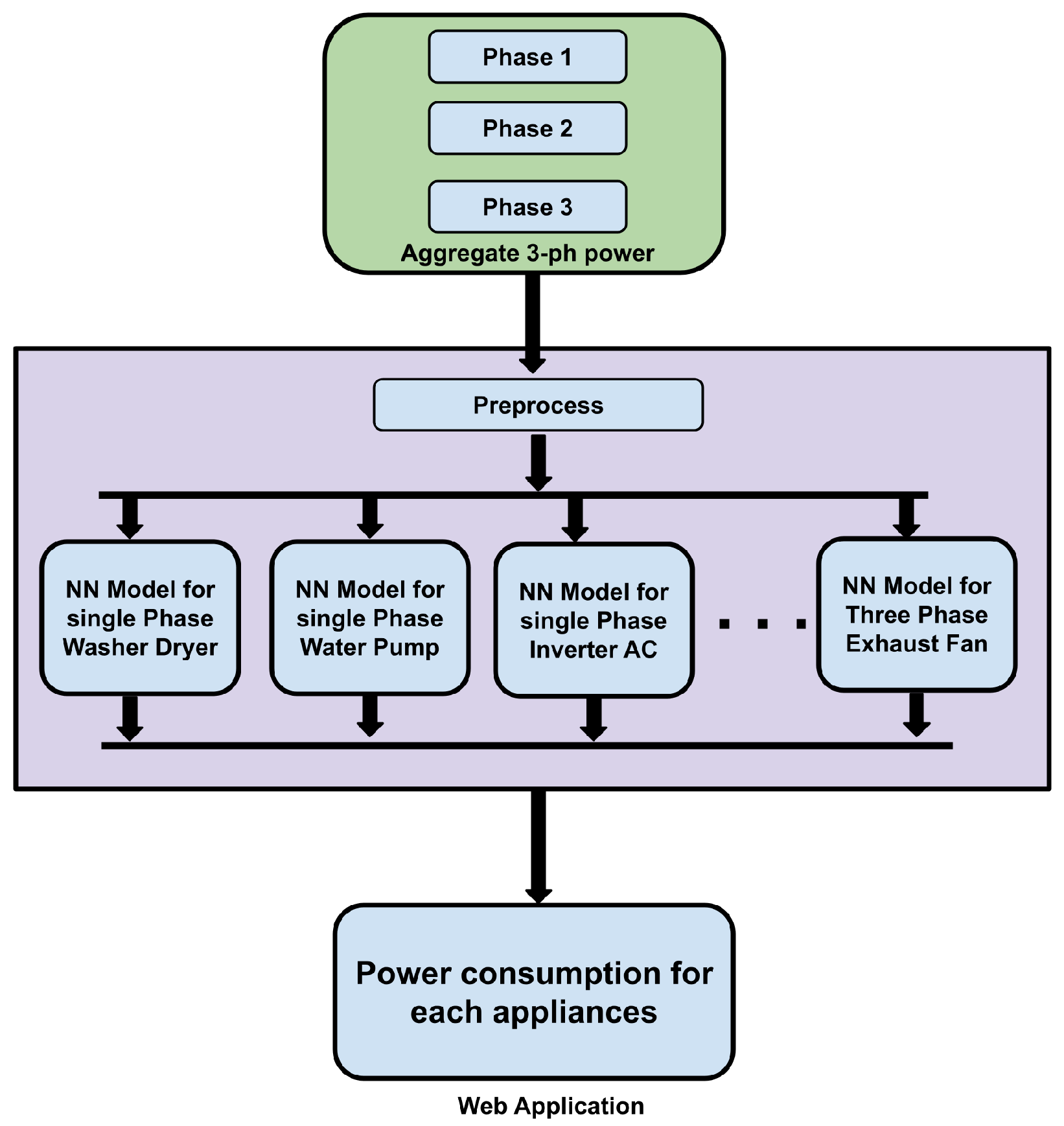
The pipeline of the proposed approach comprises two sub-models: data preprocessing and training and testing. The data preprocessing model creates the three-phase dataset and the standardizing required before the data are fed to the NN. For that, we use the NILMTK tool kit. The training and testing model uses this preprocessed data to train and test the NN. Here, we train separate NN models for each target load component. In inference, the three-phase power data that we obtain from the customer power mains are fed to these NN models so that each model predicts the power pattern of the load component it is trained to identify and classify, as shown in the following simplified Figure 1.

2.1. Data Preprocessing

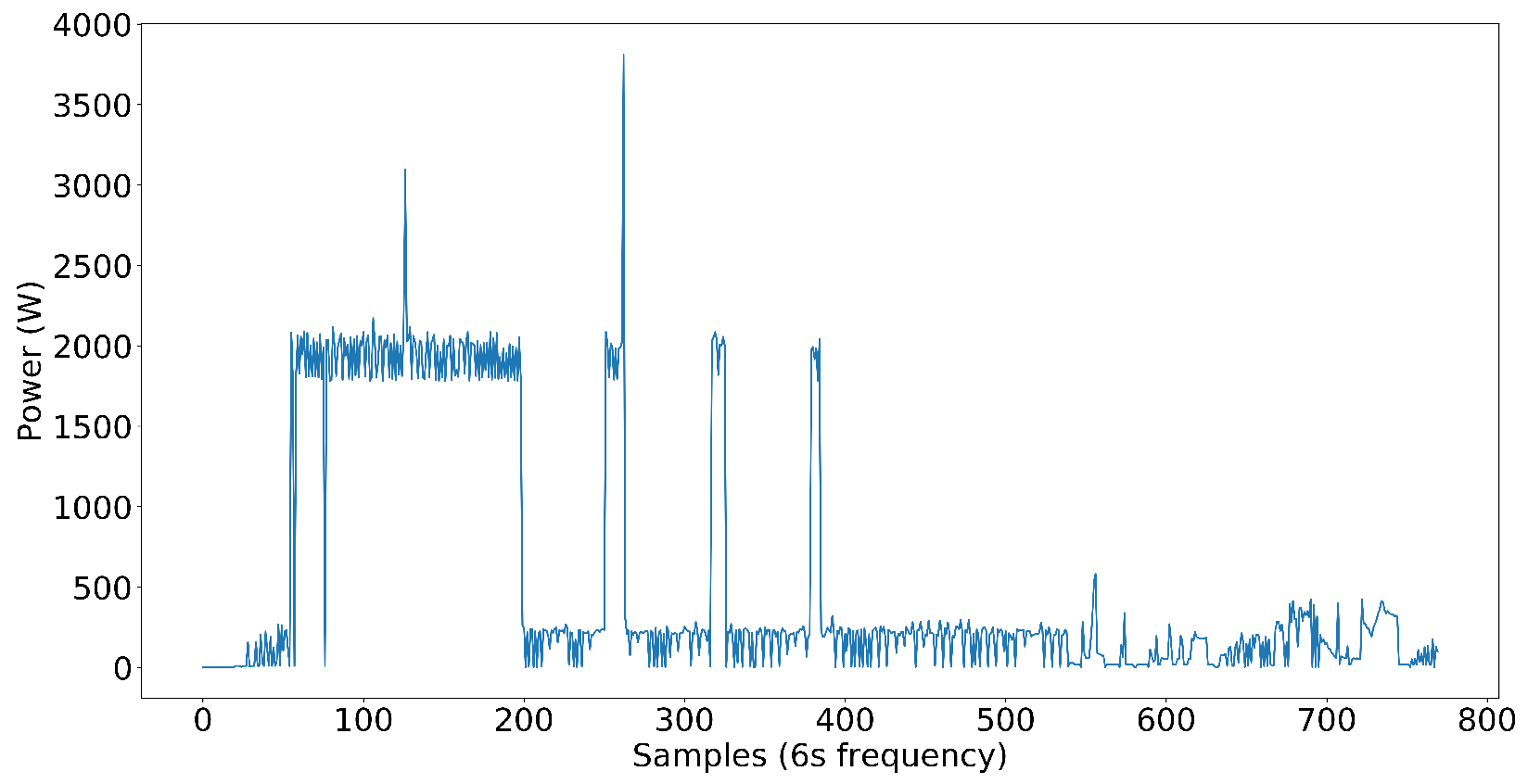
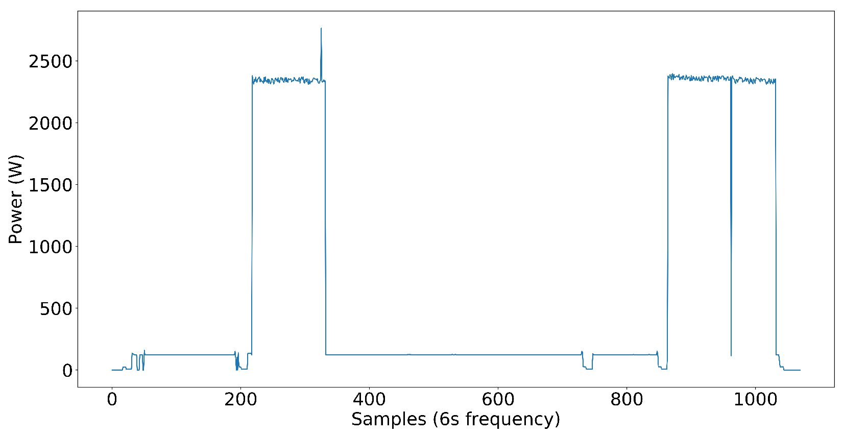
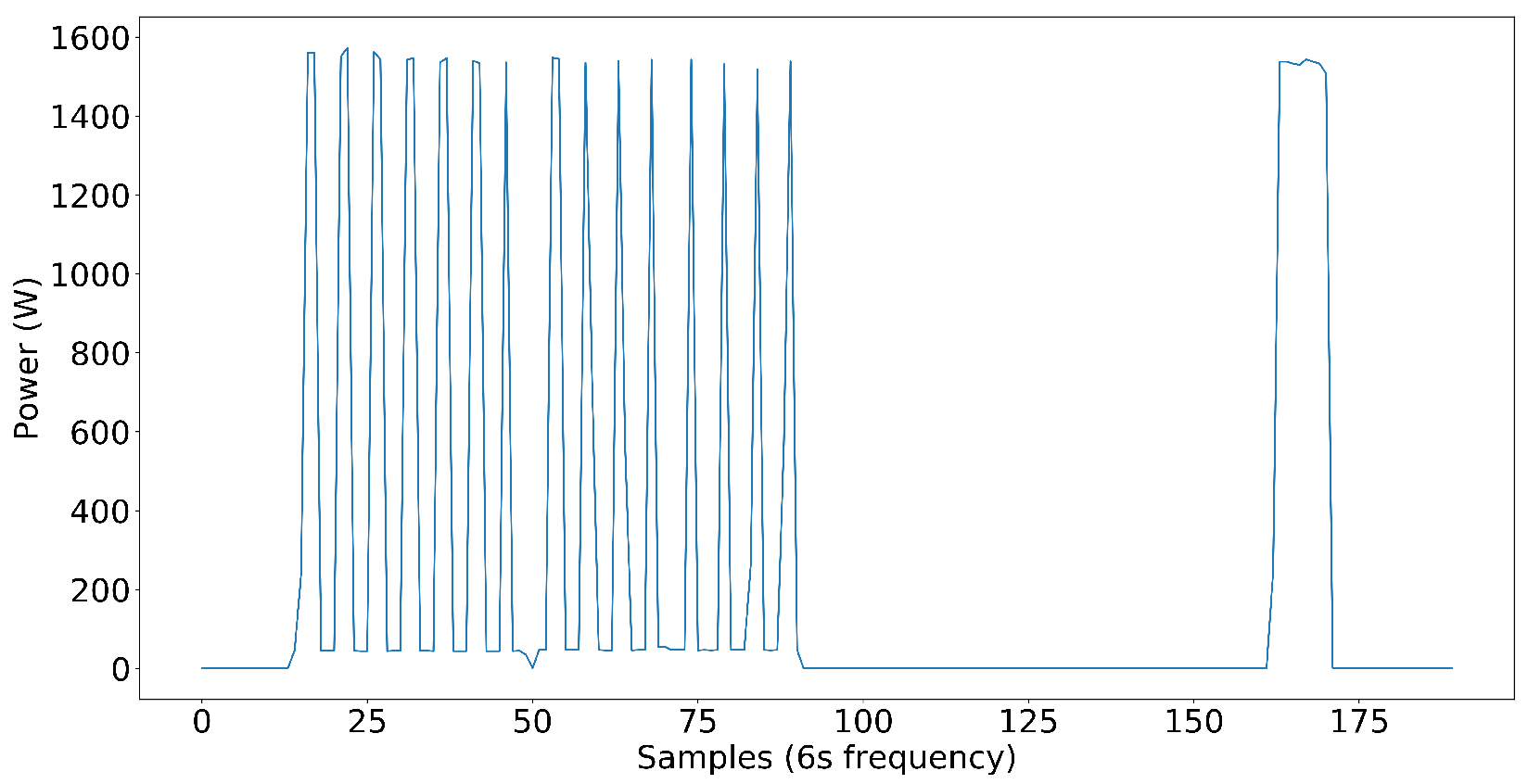
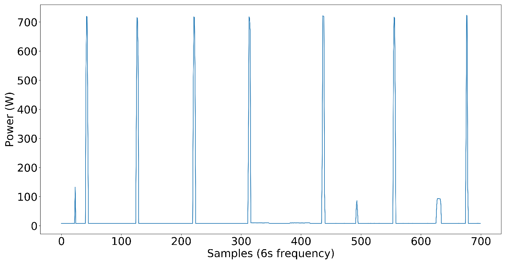
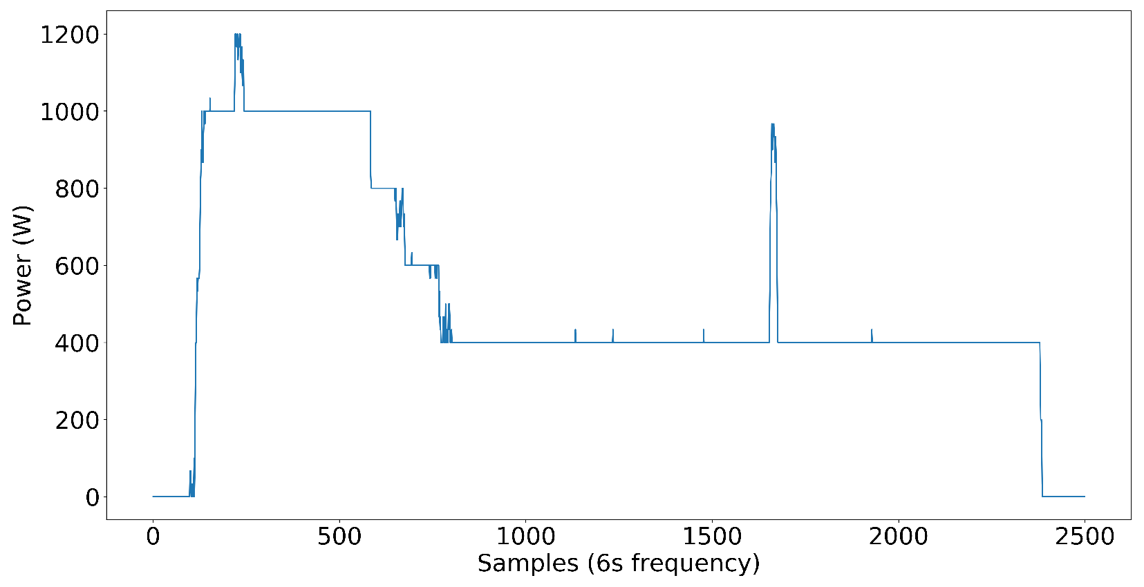
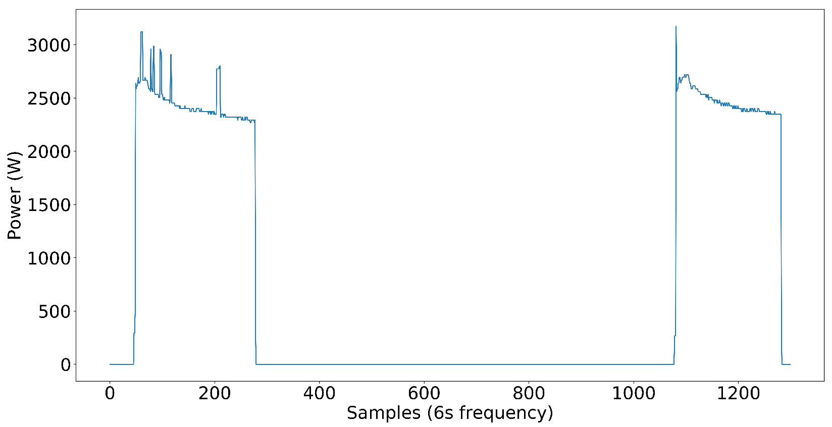
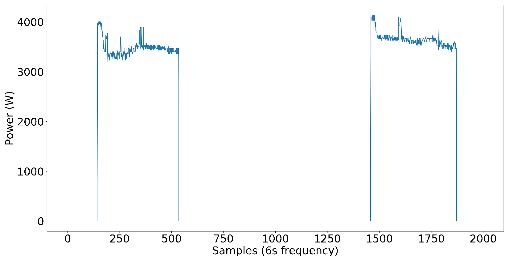
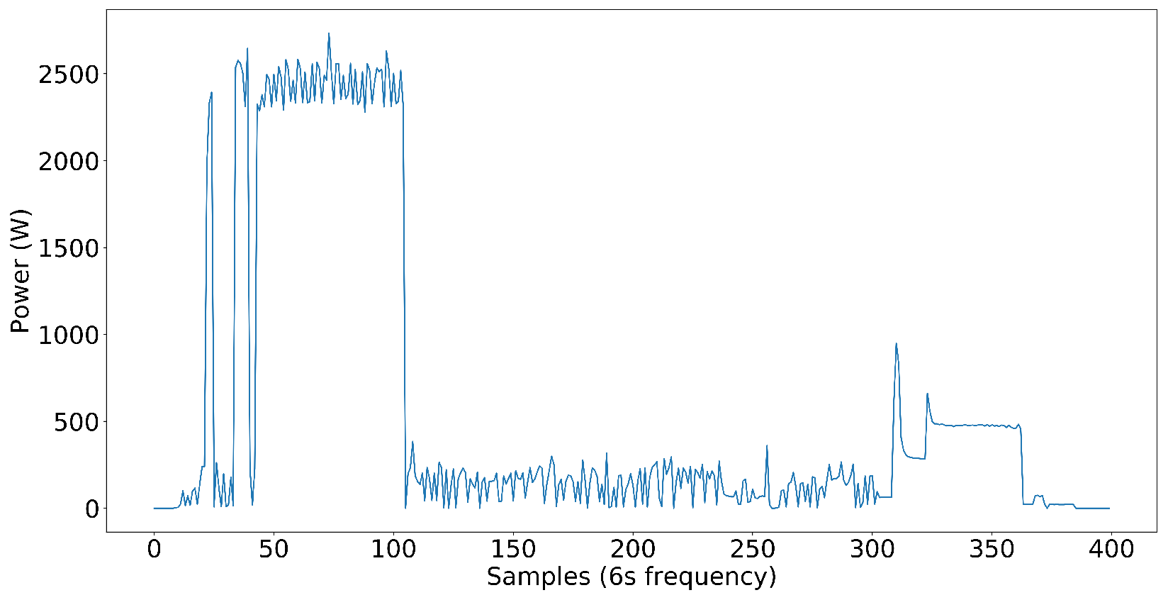
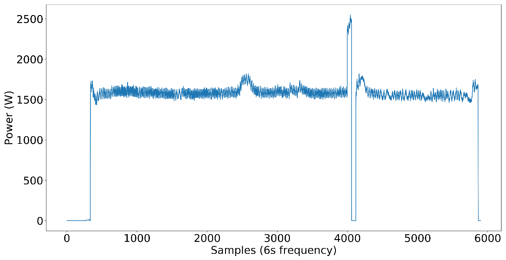
Dataset creation was significant for us since our goal was to develop an NN model that has the capability of disaggregating power into individual load components in complex power systems. For the first step, we included nine target load components in the dataset, which include a washer–dryer, dishwasher, microwave, water pump, and AC as single-phase load components and two fridges, a washing machine, and an exhaust fan as three-phase load components and power pattern are shown in Figure 2, Figure 3, Figure 4, Figure 5 and Figure 6. Later, we added inverter-type AC to test on nonlinear loads. The loads that are not high power but affect the NN model’s capability to disaggregate the power to each target load are distractor loads. Distractor loads include lights, fans, desktop computers, chargers, TVs, etc. As you can see, the dataset already included some low-power nonlinear loads without inverter-type ACs, even though we did not have any high-power nonlinear loads. It proves that the NN model performs well even in the presence of nonlinear loads in the electrical system.

For the creation of the three-phase dataset, data are collected from three online datasets, namely UK Domestic Appliance-Level Electricity (UK-DALE) [24], Industrial Machines Dataset for Electrical Load Disaggregation (IMDELD) [25], and Pecan Street Dataport [19], which are supported by the NILMTK toolkit. These datasets were selected based on their relevance, diversity, and the specific requirements of our study.

UK-DALE is a widely known dataset for load identification and classification, chosen due to its detailed appliance-level data and high sampling frequency, providing valuable insights into residential energy consumption patterns. The UK-DALE dataset contains information on the electricity consumption of five houses, including the total power demand of each house’s mains every six seconds and the power demand of individual appliances in each house every six seconds.

IMDELD is a dataset containing heavy machinery used in Brazil’s industrial sector, collected from a poultry feed factory in Minas Gerais, Brazil. This dataset was selected for its representation of industrial loads, offering a different perspective from residential datasets and aiding in the development of a robust NILM model capable of handling various load types.

The Pecan Street Dataport dataset contains circuit-level and building-level electricity data from 722 households. A subset that supports NILMTK was used due to its extensive coverage of residential energy usage and the variety of electrical appliances monitored, which enhances the diversity of our training data.

Due to the lack of online datasets representing nonlinear load components, we decided to record data locally. We selected two inverter-type ACs inside the University of Moratuwa premises to address the gap in existing datasets. Data are recorded using a Fluke 435 series-2 device and a PZEM-004T power sensor module, both with a 1 Hz sampling frequency. These data are also added to the three-phase dataset created.

We also use the NILMTK toolkit to preprocess this locally recorded data, ensuring consistency and compatibility with the online datasets. This comprehensive approach in dataset selection and data recording enhances the robustness and generalized of our NILM model across various load types and operational conditions.

The target load components we have selected cover a wide variety of loads in the commercial power systems we see today. Some loads are closer to ON-OFF power patterns, some have multi-stage power patterns, and loads like exhaust fans have continuous power patterns with small variations in power. The following figures illustrate the power patterns of each target load component we used to create the three-phase dataset.

Even though a wide variety of loads were selected to test the NN model for more complex loads, we also included loads close to similar power patterns. You can see that from the two three-phase fridges in the figures: Figure 7 and Figure 8 and three-phase washing machine and exhaust fan pattern in Figure 9 and Figure 10.

As can be observed from Figure 11, the aggregated three-phase power patterns represent:

• A very complex aggregated power pattern. This is desirable since a commercial electrical power system typically contains many loads with different power signatures.
• A noisy electrical system. Usually, this is the case with commercial power systems.
• An unbalanced electrical power system. This is the case with most industries due to highly complex electrical systems. Adding different loads to the system without proper design can lead to inherent imbalances. Even though loads are distributed among the three phases to have phase balance due to the turn ON and OFF times of loads, unbalances can occur, as explained in the introduction.

When creating the three-phase dataset, we created a Python object with the aggregated power of the three phases and each load’s power. After adding all the data, the Python object is saved in Pickle format. We followed this method to retrieve data quickly when training and testing the NN model.

Now, let us move into the NN model we have implemented. From the three-phase dataset, 75% of the data are used to train the NN model to obtain the trained weights. These weights are later loaded into the NN model with the rest of the 25% of the dataset to test our approach.

2.2. Deep Neural Network Architecture

We have tried several techniques to convince ourselves that our final NN architecture can capture any load component’s features. Because of this same reason, we created a more complex and diverse dataset. Here, we discuss our approach to give you an overview of the implemented NN architecture.

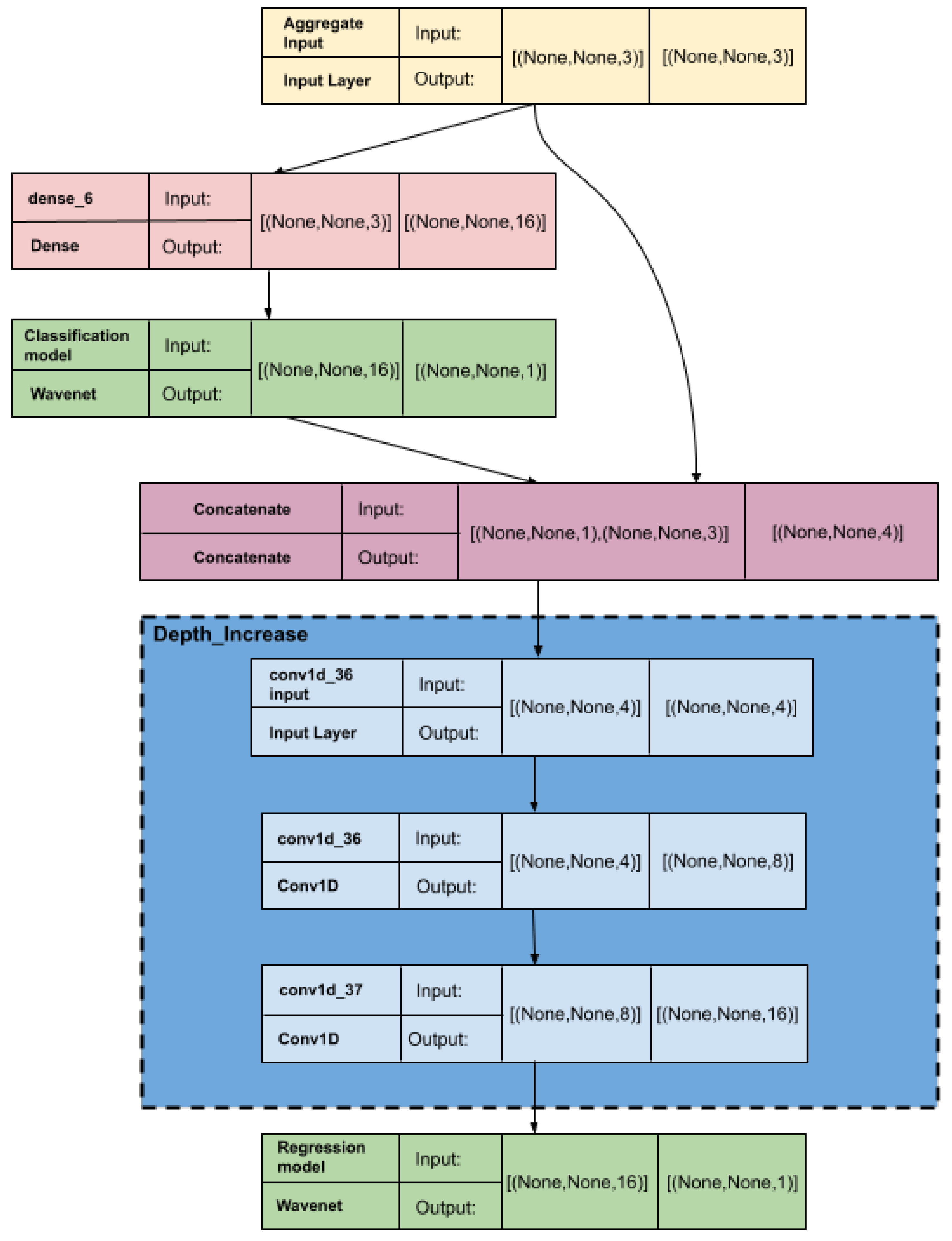
Figure 12 represents the implemented NN architecture. The input layer accepts the aggregated power data from the three phases. We also use an ON/OFF classifier to determine whether the target load component is ON or OFF before predicting the power curve using a power ON threshold to generate labels to train the classifier. The classification layer increases the model’s accuracy by predicting ON times, suppressing the power prediction by the NN model’s regression layers when the load component is OFF. The classifier’s output and the aggregate input are then fed to the concatenate layer. After concatenation, the data undergoes a series of convolution layers to extract the features. Finally, a regression layer is used to predict the power of the target load component. As Figure 12 indicates, both the classification and regression sub-models use the WaveNet architecture. When considering the final weights of the NN model for a particular load component, We use a low-cost ensemble technique to obtain more generalized model weights. Here, we used a sequence-to-sequence approach instead of a sequence-to-point approach [18].

2.2.1. WaveNet Architecture

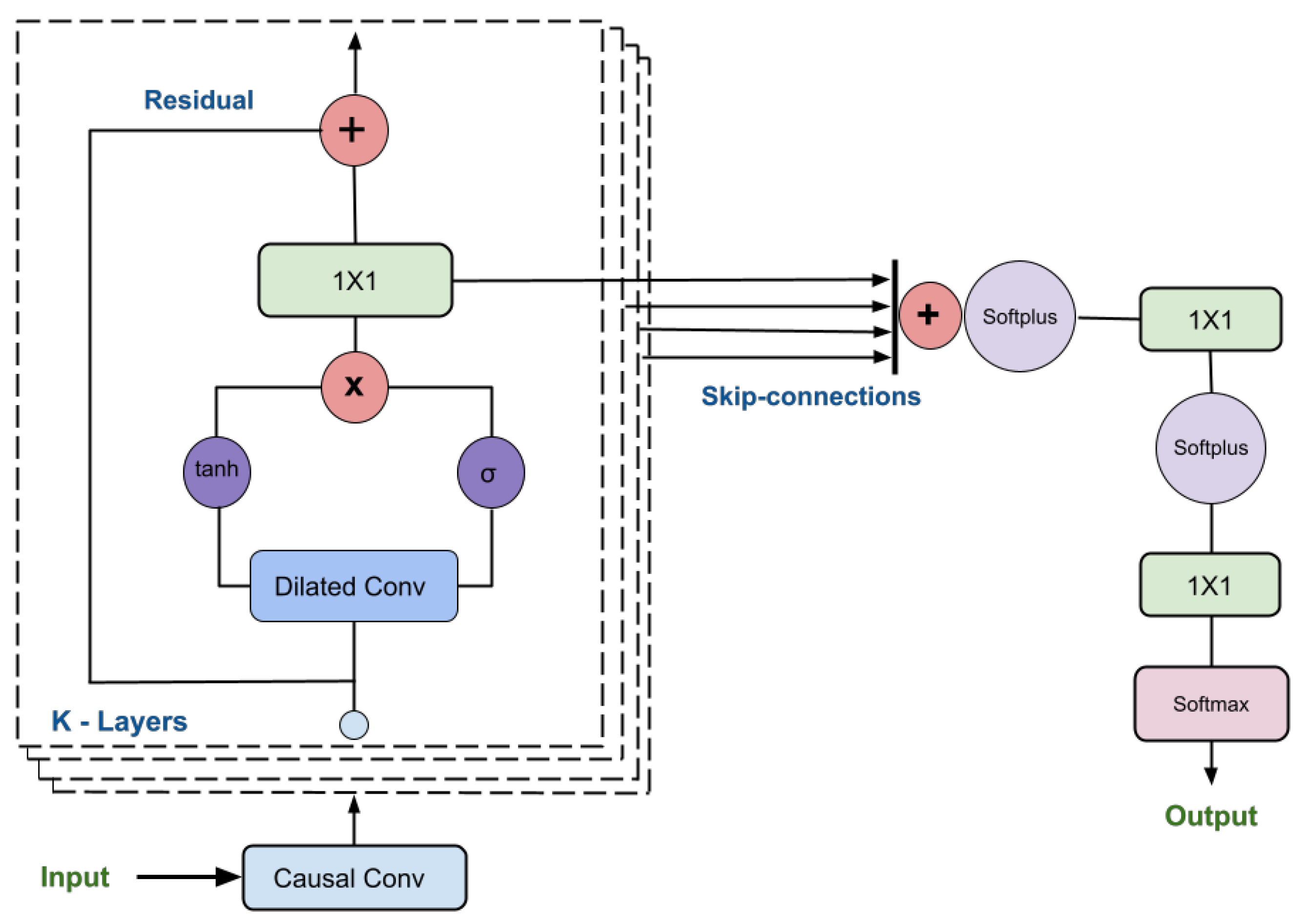
Figure 13 represents the WaveNet architecture we used to implement the classification and regression model layers. We selected WaveNet because it effectively learns long-range temporal dependencies in data through dilated and causal convolutions. Dilated convolutions capture long-term features and incorporate larger context information without significantly increasing the number of parameters, making it suitable for tasks such as image segmentation and sequential data analysis. Causal convolutions ensure that the output at each time step only depends on previous time steps, mimicking a causal relationship crucial for time series analysis. Previous researchers used models like Sequence-to-Sequence, Sequence-to-Point, and Long Short-Term Memory (LSTM) for non-intrusive load monitoring. However, these older architectures are optimized for natural language processing and may not be ideal for power pattern recognition. We found WaveNet to be particularly suitable for this purpose, effectively capturing signal variations with noise and distinct features and outperforming the previously mentioned models, especially for three-phase devices. We further enhanced the WaveNet model using ensemble techniques, which significantly improved performance. Given these successful results across various devices, we chose to stick with this architecture.

Here are some other main components and characteristics of the WaveNet architecture:

• Residual Connections: WaveNet utilizes residual connections inspired by the ResNet architecture to improve the flow of information through the model. Residual connections enable the model to retain and propagate important information through the layers, which helps alleviate the vanishing gradient problem and speed up training.
• Gated Activation Units: WaveNet employs gated activation units, specifically the combination of a sigmoid and a hyperbolic tangent activation function, to control the flow of information within the network. This gating mechanism allows the model to selectively update and pass information through the layers, enhancing the modeling capabilities of the network.
• Skip Connections: Skip connections, similar to the residual connections, are used in WaveNet to create shortcut connections between the early and late layers of the network. These connections enable the model to capture both short-term and long-term dependencies simultaneously, facilitating the generation of coherent and realistic audio samples.

2.2.2. Low-Cost Ensemble Technique

Ensembling is a technique used in NNs to improve the performance and generalization of the model by combining predictions from multiple individual models. It leverages the idea that multiple models with diverse characteristics can provide more accurate and robust predictions than a single model. There are different methods to perform ensembling in neural networks, but two commonly used techniques are:

• Model averaging: In model averaging, multiple individual models are trained independently on the same dataset using different initializations or hyperparameters. During prediction, the outputs of all models are averaged or combined in some way to obtain the final prediction. This approach helps reduce the impact of individual model biases or overfitting and improves overall performance.
• Model stacking: Model stacking, also known as a stacked generalization, involves training multiple individual models on the same dataset, similar to model averaging. However, instead of directly combining their predictions, a meta-model is trained to learn how to best combine the predictions from the individual models. The meta-model takes the outputs of the individual models as inputs and learns to make a final prediction based on them. This approach allows for more sophisticated combination strategies and potentially captures more complex relationships between the individual models.

Ensembling techniques can be applied to different types of neural networks, including feed-forward networks, convolutional neural networks (CNNs), and recurrent neural networks (RNNs). It is important to note that ensembling requires training and maintaining multiple models, which increases computational resources and training time. However, the improved performance and generalization often justify the additional complexity.

Our Low-Cost Ensembling approach, shown in Figure 14, involves the first technique by continuously training our same NN model. After convergence, we obtain multiple models with high accuracy and average them to obtain the final model weights. The reason it is called low-cost is that we only use one model to obtain multiple model weight combinations, which saves a lot of computational resources. By combining weights from multiple models, we could reduce errors and improve the model’s overall accuracy. Ensembling provided us with several benefits:

• It could help capture different aspects or patterns in the data that a single model may miss.
• Improved generalization: Ensembling helps reduce overfitting by incorporating diverse models. Each model weight combination may have its strengths and weaknesses, and ensembling can mitigate the impact of individual model weaknesses, leading to better generalization on unseen data.
• Enhanced robustness: Ensembling can improve the robustness of the model by reducing the impact of outliers or noisy data points. Outliers may affect the predictions of individual models differently, but ensembling combines the predictions, reducing the influence of individual errors.
• Confidence estimation: Ensembling can provide estimates of prediction confidence or uncertainty. By considering the variability of predictions across different models, ensembling can offer insights into the reliability of the predictions.

2.3. Web Application

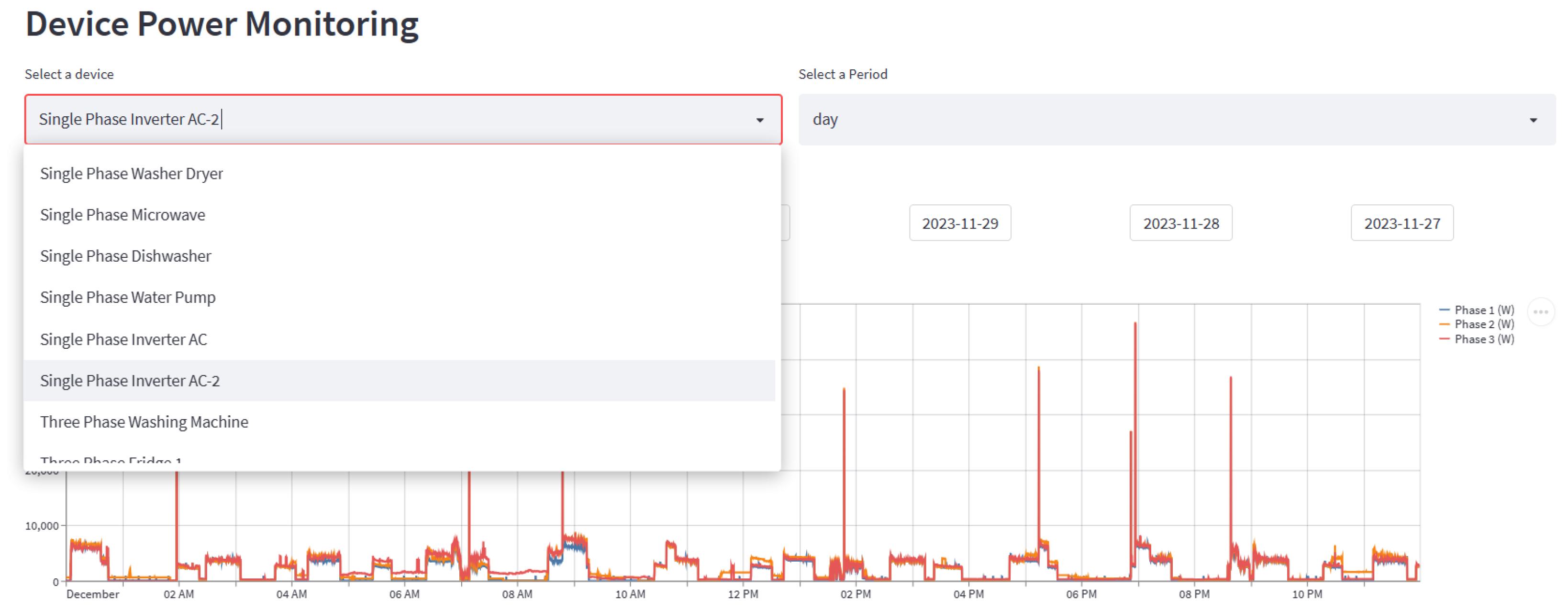
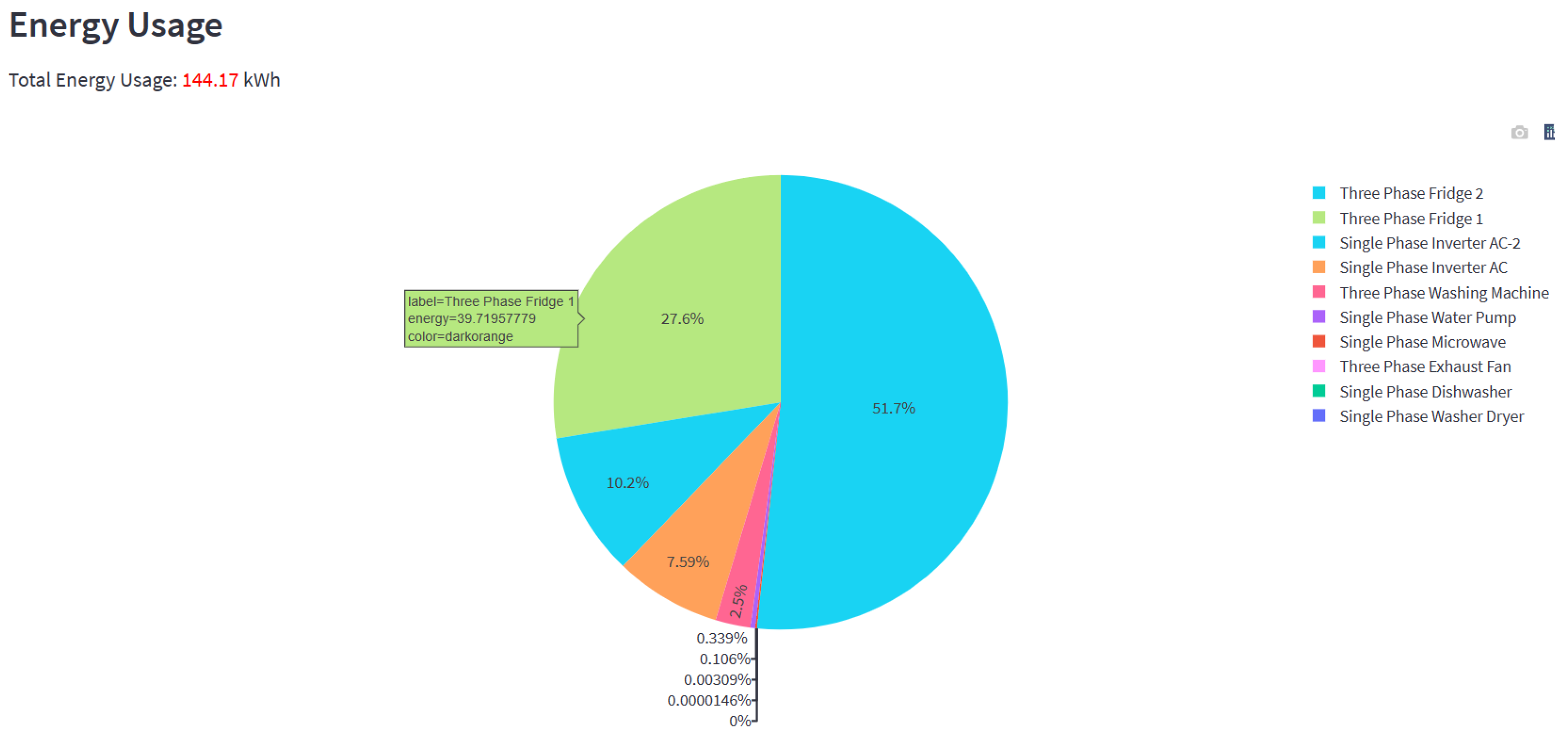
The following Figure 15, Figure 16 and Figure 17 represent the developed web application. As shown in Figure 15, the user can select the load component that needs to be monitored and the time period. The graph shown in Figure 15 is the three-phase power, which should be coming from the sensor installed at the user’s power mains, ideally. According to the user selection, the NN model, which runs in the backend, predicts the power pattern for the selected load component. Energy usage for the load component chosen for the set period is also shown. Users can zoom in and out of these graphs and view the power at any time. The pie chart shown in Figure 17 shows how each high-power load component in the system consumed energy.

Here, the load component is selected as “Single-Phase Inverter AC-2” and the period as “day”. Users can also select “month” as the period to see the energy usage for the month. This gives a WiFi-like approach by empowering users with information to gain control over their electrical energy usage.

3. Experimentation and Results

This research is unique and innovative since it addresses quite challenging aspects of NILM in today’s world. Our final dataset, which is used to train and test the NN model, is very complex, and with the added randomness due to the nonlinear loads, it became quite challenging to have good accuracies for the load components in the system. While addressing these challenges, we also ran the NN in the web application’s backend to experiment with the NILM on the user experience. We were able to give the users WIFI-like awareness, as explained earlier.

3.1. Three-Phase Dataset

Initially, we tested our model with only limited loads. As explained earlier, the dataset contains load components with somewhat similar power signatures, up to the load components with highly random power patterns. We also made sure to use NILMTK to process the datasets that we obtained online. We synthesized only the locally recorded data, and we made sure to separate the training and testing data so that testing data are new to the NN model.

3.2. Nonlinear Loads

We wanted to test our NN model for the nonlinear load components as well. However, due to the unavailability of data online, we went with collecting data locally. For that, we used a PZEM-004T power sensor to record the data continuously for 12 days. As a highly nonlinear load component, we selected an inverter AC manufactured by LG located at the Transport and Logistics Department of the University of Moratuwa. After carefully examining its power pattern, we selected this AC to confirm its highly nonlinear operation. You can see its power pattern in Figure 18. As can be seen from Figure 18 unlike the previous non-inverter-type AC shown in Figure 6, its power pattern is very complex. When it comes to this inverter-type AC, it is a load component that can run at any power in a specified power range, which goes under Type-IV as described in [14]. The inverter AC we have considered can run even at a hundred watts, but when it is running at full power, it is about 2 kW. Also, its power pattern is highly dependent on the outside weather. This behavior shows us how complex the inverter AC we have considered is. Later, under the topic “Inverter-type AC integration”, we mainly assess the impact of this inverter AC integration on the existing dataset.

3.3. Evaluation Matrices

To assess the model’s performance and validate the accuracy of its predictions, we employ three essential metrics: mean absolute error (MAE), mean squared error (MSE), and F1-score. The mean absolute error (MAE) quantifies the average magnitude of the errors between the observed and predicted values within a dataset. The calculation of MAE is carried out by applying Equation (1). The mean squared error (MSE) assesses the average of the squared differences between predicted and observed values within a dataset. The calculation of MSE is carried out by applying Equation (2), as shown below.

$$MAE={\displaystyle \frac{1}{T}}\sum _{t=1}^T|y_t-{\widehat{y}}_t|$$

(1)

$$MSE={\displaystyle \frac{1}{T}}\sum _{t=1}^T{|y_t-{\widehat{y}}_t|}^2$$

(2)

where

$${\widehat{y}}_t=The prediction of the model at time t$$

$$y_t=The actual power consumption at time t$$

The Following two equations help to calculate the F1_Score.

$$Precision={\displaystyle \frac{TP}{TP+FP}}$$

(3)

$$Recall={\displaystyle \frac{TP}{TP+FN}}$$

(4)

$$F1\_Score=2·{\displaystyle \frac{Precision·Recall}{Precision+Recall}}$$

(5)

where

$$TP=The model prediction indicates the loadcomponent$$

$$is ON,when the loadcomponent is actually ON$$

$$FP=The model prediction indicates the loadcomponent$$

$$is ON,when the loadcomponent is actually OFF$$

$$FN=The model indicates the loadcomponent is OFF$$

$$when the loadcomponent is actually ON$$

Predicted values are classified as ON or OFF using a threshold value; values over the threshold are classified as ON, and values below it as OFF. The needs particular to the application are used to calculate the suitable threshold value. For instance, we chose a threshold value of 0.25 for most of the load components. The F1 score helps assess classification algorithms, especially for imbalanced datasets, as it integrates precision and recall into a single value. Recall is the percentage of genuine positive outcomes among actual positive outcomes, whereas precision is the percentage of real positive outcomes among anticipated positive outcomes.

3.4. Inverter-Type AC Integration

This study additionally presents a method to enhance the efficacy of non-invasive load monitoring (NILM) in commercial buildings through the integration of nonlinear load components into the current model. Because these load components can save energy, their integration into power systems has much potential. Two inverter-type AC units were used in this investigation, and pertinent data were collected as previously discussed. With notable performance measures for both Inverter AC 1 and Inverter AC 2, the preliminary results show promise.

3.5. Results

The Kaggle platform was employed in our study to train and test our model. To improve computational efficiency, we specifically used the GPU P100 accelerator accessible on the Kaggle platform. We conducted experiments on Kaggle to achieve the results that are shown here.

We systematically explored various hyperparameters to optimize performance for appliance prediction. Our exploration ranged from simple to more complex models, varying sample sizes, depths, the number of WaveNet layers, and initial learning rates. Through manual iteration and parameter tuning, we identified two sets of hyperparameters that yielded promising results. Notably, these parameters consistently demonstrated efficacy across different appliances. The evaluation metrics employed include training validation mean squared error (MSE), mean absolute error (MAE), and training time.

The accompanying

Table 1. Hyper Parameters: Analysis.

Appliance	Hyper Parameter 1			Hyper Parameter 2
	MSE	MAE	Training Time (S)	MSE	MAE	Training Time (S)
Inverter AC 1	0.00471	0.01578	741.51	0.00162	0.00679	965.925
Inverter AC 2	0.04241	0.12931	744.56	0.04360	0.13068	939.32
Washer–Dryer	0.00624	0.01079	717.77	0.00943	0.01326	957.73
Exhaust Fan	0.04882	0.03107	569.19	0.05176	0.02709	673.41
Fridge 2 (3-Phase)	0.00112	0.00777	706.49	0.00129	0.00701	828.73

illustrates the performance of the two inverter AC units, one single-phase device, and two three-phase devices, alongside other appliances. For Hyperparameter Set One, with a sample size of 42,000 and an initial learning rate of 0.01, the model depth was set at 16, with six WaveNet layers. Conversely, Hyperparameter Set Two featured a sample size of 42,000, an initial learning rate of 0.01, a depth of 20, and eight WaveNet layers. Despite exploring various configurations, these two sets consistently outperformed others in terms of predictive accuracy and training time.

A comparative analysis presented in the table suggests that Hyperparameter Set Two generally outperformed Hyperparameter Set One, albeit with exceptions noted for the washer–dryer appliance. Notably, while Hyperparameter Set Two exhibited superior predictive performance, it incurred significantly longer training times. Thus, based on our research findings, we elected to adopt Hyperparameter Set One as our final configuration.

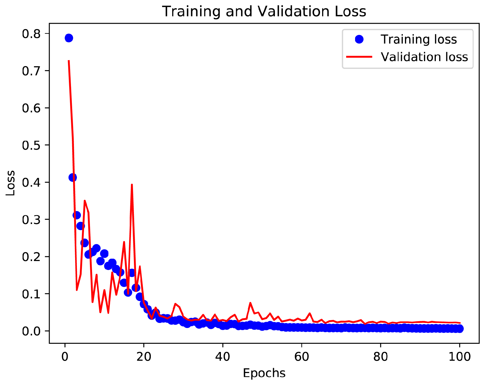
The study of the learning curve offers insightful information about how each appliance behaves throughout training. Examining the learning curves allows us to determine whether overfitting or underfitting is occurring. The training and validation loss curves must be closely examined for this analysis. We can successfully optimize the training process using such an approach.

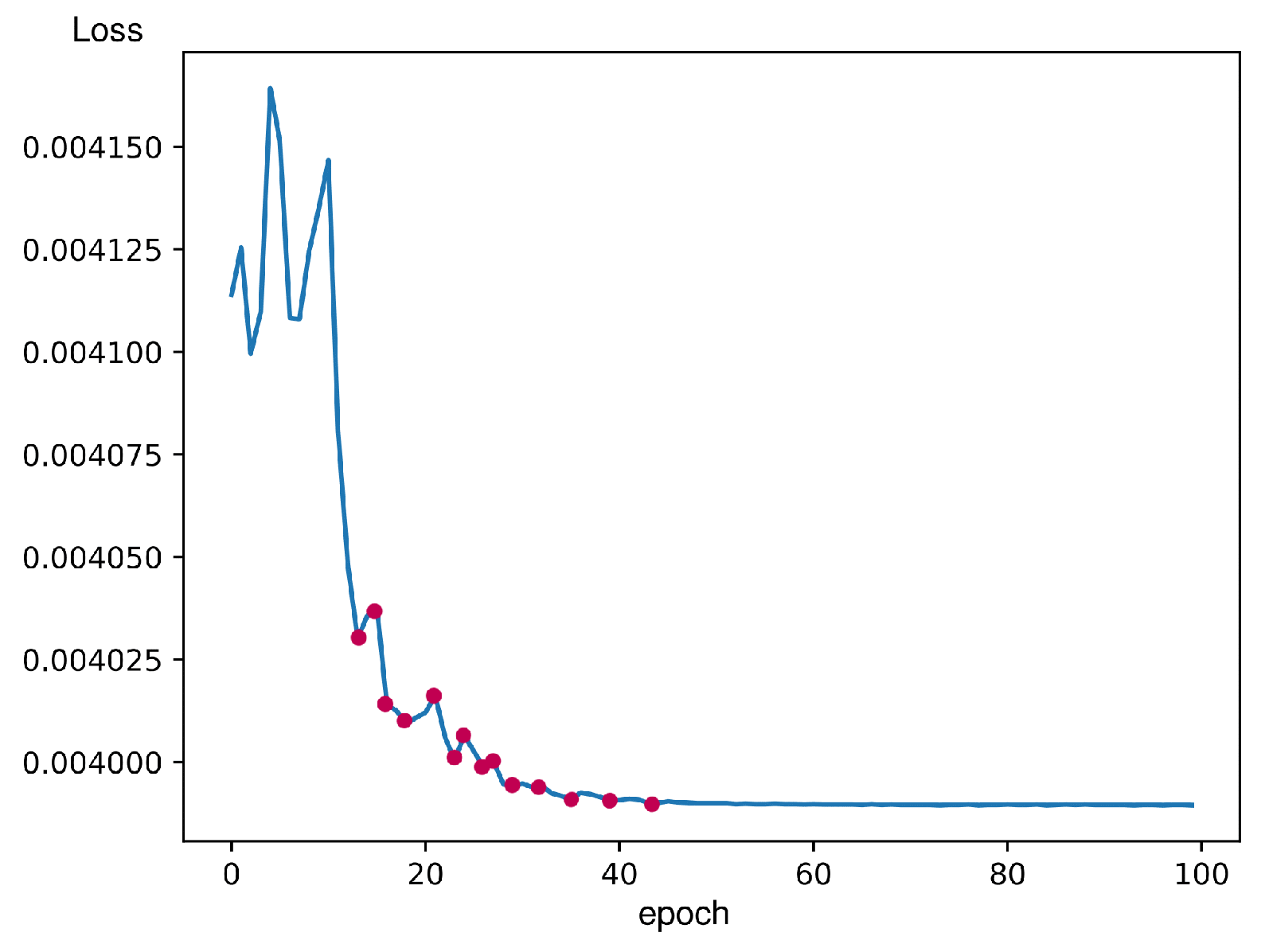
We conducted a comprehensive analysis of the learning curves for all appliances, focusing initially on the single-phase microwave device as shown in Figure 19. Remarkably, similar learning curves were observed across all other appliances studied. In this learning curve, you can observe the fluctuation in the beginning that happens because of the ADAM optimizer. Adam changes the learning rate according to the observed gradient, resulting in a gradual reduction of the learning rate over time. The fluctuation of validation loss decreases when the learning rate decreases. This scenario explains the adaptive nature of the ADAM optimizer and its impact on the training dynamics.

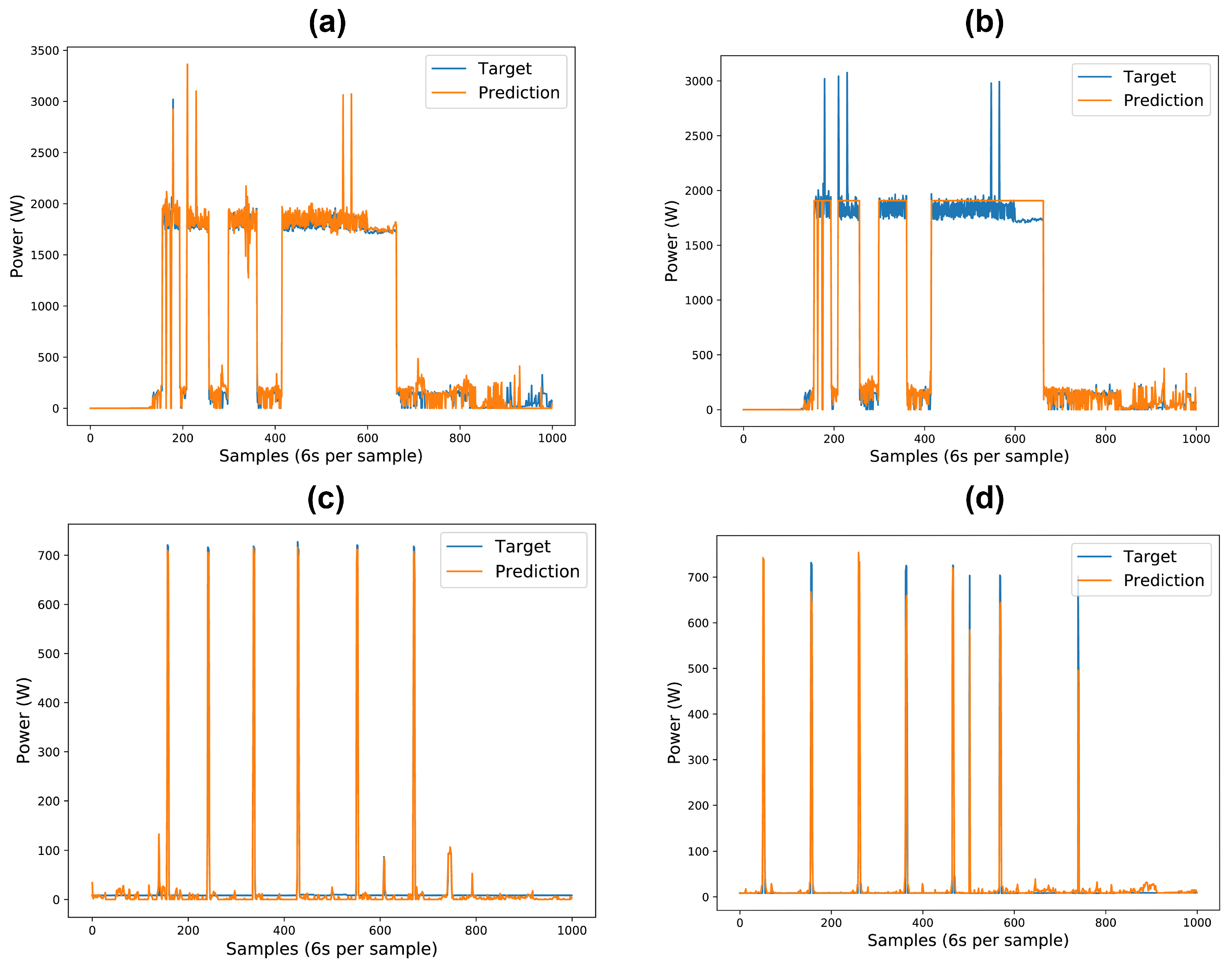
The deep NN model could accurately predict the single-phase and three-phase load components’ power patterns for the three-phase test dataset. Some predictions done by the NN model are shown in Figure 20, Figure 21, Figure 22, Figure 23 and Figure 24. The test dataset includes the last 25% of the three-phase dataset, which adds up to three months. The validation of results comprises the utilization of classification and regression model losses. Specifically, validation classification model loss is a metric to assess the classification model’s performance during the training process’s validation phase. Similarly, validation regression model loss is employed as a metric to evaluate the regression model’s performance during the training process’s validation phase. Detailed load-specific validation classification loss and validation regression loss values are presented in

Table 2. Classification and Regression Validation Loss.

Load Component	Validation Classification Loss	Validation Regression Loss
Dish Washer	2.45 × 10−8	7.75 × 10−3
Microwave	2.60 × 10−8	1.47 × 10−2
Washer-Dryer	2.90 × 10−8	4.76 × 10−3
Water Pump	2.38 × 10−8	7.23 × 10−1
Fridge 1 (3 Phase)	4.09 × 10−2	1.24 × 10−2
Fridge 2 (3 Phase)	1.09 × 10−2	5.33 × 10−3
Washing Machine (3 Phase)	2.66 × 10−8	8.87 × 10−3
Exhaust Fan (3 Phase)	2.08 × 10−2	2.48 × 10−3

.

Mean absolute error values for the load components are provided in

Table 3. Mean Absolute Error Values for the Load Components.

Load Components	MAE
Dish Washer	1.13 × 10−2
Microwave	1.35 × 10−2
Washer Dryer	1.17 × 10−2
Water Pump	7.88 × 10−3
Fridge 1 (3 Phase)	1.62 × 10−2
Fridge 2 (3 Phase)	9.17 × 10−3
Washing Machine (3 Phase)	1.92 × 10−2
Exhaust Fan (3 phase)	8.09 × 10−2

. The preliminary results of nonlinear devices exhibit promise, with noteworthy performance metrics for both Inverter AC 1 and Inverter AC 2. Specifically, for Inverter AC 1, the mean absolute error is 7.88 × 10⁻³, accompanied by a validation classification loss of 4.35 × 10⁻³ and a validation regression model loss of 1.19 × 10⁻³. Meanwhile, for Inverter AC 2, the mean absolute error is 1.80 × 10⁻², with a validation classification loss of 4.48 × 10⁻¹ and a validation regression model loss of 5.30 × 10⁻². The visualization of our model predictions is illustrated in Figure 25 and Figure 26.

Upon integrating the inverter-type load component, we observed a marginal reduction in prediction accuracy for specific load components, namely the washer–dryer and water pump. This underperformance, as illustrated in Figure 27, can primarily be attributed to the integration of inverter-type devices, which do not exhibit specific on-off power patterns. Instead, they generate various power patterns, causing the model to misinterpret signals from other devices, leading to errors in device identification and classification. To address this issue, we recorded additional inverter-type device data locally to enhance the model’s learning. The presence of inverter-type devices introduced marginal errors, particularly affecting devices with small variations like water pumps and washer-dryers. However, even with the inclusion of these marginal errors, our model still delivered very good results. Future implementations will benefit from the continued recording and inclusion of diverse inverter-type device data to mitigate these issues and further enhance model accuracy.

4. Conclusions

In this research, we have developed a robust, Non-Intrusive Load Monitoring (NILM) technique utilizing a Convolutional Neural Network with the WaveNet architecture. Our model is versatile and suitable for deployment in both domestic and commercial buildings. Through rigorous experimentation and the implementation of inventive solutions, we have proactively tackled the following challenges for the future.

• Energy Disparity: The higher consumption of three-phase load components can overshadow the power usage of smaller single-phase load components, potentially distorting accurate load monitoring.
• Customized Data Gathering and Model Training: Each customer’s building necessitates tailored data collection and model training, introducing logistical complexities.
• Aging Load Patterns: Our research has thoughtfully addressed aging load components’ evolving power consumption patterns over time.
• Load Distinction Challenges: Our NN model could accurately distinguish between similar load components using small differences in power signatures.
• Nonlinear Loads: Accurately predicted the power patterns of the two inverter-type ACs. Also identified that the integration of nonlinear load types may marginally affect overall accuracy, prompting consideration.

Our model has outstanding performance in both commercial building and home applications, showcasing great precision in load identification, especially when confronted with nonlinear load components. The exceptional efficiency and brief training period of this technology result in practical advantages. In our study, we employed ten separate devices with varying levels of distraction to evaluate the effectiveness of our concept. The model effectively processed datasets that were both noisy and imbalanced, accurately simulating real-world scenarios. In our study, we used power data with a 6-s frequency. However, our model is designed to be flexible and is expected to perform well with data frequencies ranging from 1 s to 10 s. The effectiveness of the model may decrease if the data frequency is too low, leading to noisy data, or too high, resulting in insufficient features for the model to utilize effectively. This range provides a robust framework for various data granularities while maintaining performance.