Analysis of the Relationships between Variables and Their Applications in the Energy Saving Field

Abstract

Energy saving is an important measure to promote social green transformation. The traditional energy-saving ideas usually only focus on a specific loss, and seldom consider the possible relationship and influence among various losses. In relatively complex energy-using systems, there are often many kinds of losses, and each loss may have many influencing factors. There may be some relationship between these losses and the influencing factors. To solve this problem, this paper presents an analysis method of the variable association in multi-variable systems. First, the basic relationships between variables and the representation methods are discussed. The basic concept of a path between variables is given, and the analysis method of variable association based on path statistics is provided. This paper focuses on the analysis of the influencing factors and paths of the observed variables, as well as which observed variables will be affected by a control variable. Then, based on the correlation matrix, the quantitative analysis method of the influence between variables is given. Variable correlation analysis is innovatively applied in the field of energy saving to determine the correlation of losses through variable associations, guiding the preliminary screening of energy-saving measures and analyzing the collateral effects of these measures. Based on the correlations between energy losses, a scientific process for formulating energy-saving measures is proposed. The variable correlation analysis method proposed in this paper is a generalized method, which can judge the correlation between variables from the perspective of theoretical analysis and avoid the dependence on data. In addition to good applications in the field of energy conservation, it can also be widely used in construction, transportation, climate change, and other fields. The proposed energy-saving ideas take into account the intensity of influencing factors on loss and the correlation between loss, which improves the effectiveness of energy saving measures.

1. Introduction

Energy saving is the “first energy source” [1], with the intensification of the global energy crisis and the improvement of environmental protection awareness, energy conservation has been an area of concern. Energy saving is an important means to promote a carbon peak and carbon neutrality [2]. Energy conservation and emission reduction have emerged as crucial topics of enduring significance, both presently and in the long term. Adopting a systemic approach to energy-saving serves as the pivotal point for enhancing energy utilization efficiency [1].

Many scholars have conducted research on energy consumption and energy efficiency at the macro level. Researchers in [3] point out that researching the influencing factors and trends in energy structure has become the foundation for policy formulation. The national indicators proposed by Helmut Haberl [4] can predict energy demand and carbon emissions. In [5], a threshold model is established to examine factors influencing energy consumption, finding that technological advancements significantly contribute to energy savings. In [6], the factors affecting energy efficiency are proposed to be categorized into economic and social factors, as well as natural environmental factors, where the economic and social factors represent the genuine potential for energy savings that can be achieved. Researchers in [7] suggest dividing the influencing factors of energy efficiency into innate factors and acquired factors, which is of great significance for reducing energy loss and improving energy efficiency. In order to clarify the specific energy consumption of energy-using industries, existing studies usually use machine learning [8,9], clustering techniques [10,11], and regression analysis [12] to predict energy consumption and analyze its influencing factors.

Many industries have made efforts in energy conservation, with most energy-consuming enterprises achieving this goal through the energy-using process control or energy supply control. A secondary optimization strategy aims to enhance energy efficiency by manipulating the train’s arrival time to either advance or delay its scheduled arrival, thereby optimizing overall energy consumption [13]. Researchers in [14] delve into the investigation of the impact of rooftop photovoltaic installations on the energy consumption of buildings. In [15], a survey is presented on the most common methods of energy conservation in buildings: controlling lighting and regulating air-conditioning temperatures. Researchers in [16] suggest that new energy-saving equipment and technologies such as ground source heat pumps should be widely applied to improve building efficiency. Common energy-saving measures tend to focus on a specific energy or loss, and pay little attention to the correlation between multiple losses.

In the field of statistics, typical correlation analysis methods mainly include Granger causality analysis [17], Copula analysis [18], mutual information [19], and gray correlation analysis [20]. In the study of variable association, an adaptive variable grouping method based on Pearson correlation is proposed [21] to measure the similarity of the evolutionary trend in associated variables; however, this method may increase the complexity of large-scale optimization problems. Current studies pay more attention to the association rules among random variables, and estimate the potential association relationship between variables from a probabilistic point of view by analyzing a large amount of data, but this method cannot describe the exact relationship between variables, while the size of the database, and the number of extraneous and redundant variables will affect the accuracy of the analysis.

The development of digital and information technology has a significant impact on energy-saving and consumption reduction [22,23]. Before formulating energy-saving measures, it is usually necessary to collect a large amount of energy consumption data and monitor the changes in these data in real time [24,25]. Zhou and Razak [26,27] proposed a building energy consumption prediction model based on deep learning and machine learning. In [28], transfer learning is applied to improve the feasibility and robustness of data-driven solutions for individual buildings. Tian [29] proposes a theoretical framework of data-driven building energy consumption analysis and energy-saving design, and utilizes a Bayesian network model to identify the distribution and variation patterns of building energy consumption. These methods require a high degree of data completeness and extensive experience in designing parameters. In addition, energy saving analysis based on large amounts of data can only be used as a post hoc analysis, after the system is constructed and operated, as it takes time to collect enough data for analysis. In order to obtain data from energy-using systems, additional monitoring systems need to be installed, increasing the cost of installation, data collection, and storage.

The study in [30] proposes an optimum energy-saving technology combination suitable for a building based on a multi-objective optimization model, aiming to achieve optimal energy efficiency. Ouyang and Ju [31] formulated several mathematical models of self-saving and shared saving modes, and deduced the optimal production quantity strategy as well as the optimal unit energy saving ratio. The selection of energy-saving measures is frequently guided by the effect of energy saving, and the influence mechanism and scope of action of different energy-saving technologies are rarely discussed, which leads to the lack of the scientific selection of energy-saving measures.

Multiple variables in the energy use system may be interrelated [32], leading to the situation where energy-saving measures taken for one loss may also impact other losses [33]. At this point, the overall impact of the measure on the system has to be fully assessed to see whether the overall energy-saving effect of the measure meets the expectations, and whether it is necessary to replace the measure or take auxiliary measures.

This paper introduces a variable association analysis method, grounded in systematic energy use principles, to identify loss influencing factors and examine potential loss couplings. For systems with explicit mathematical models, the associations between variables can be directly determined. Based on the intensity of the factors and the correlation between losses within the energy-using system, two energy-saving measures are proposed to assist in planning energy usage schemes prior to the construction of the energy system.

The primary objective of this paper is to propose a methodology for analyzing and describing the correlations among variables. On this basis, we focus on which control variables will affect an observed variable, which observed variables will be affected by a control variable, and the paths of the effects. This paper expounds on the application of variable correlation analysis in the realm of energy conservation, and presents a scientific methodology for devising effective energy-saving measures.

2. Associations between Variables and the Description Method

2.1. Path and Variable Association Diagram

To analyze the interaction between variables, a “variable association diagram” is used to show the connection relationships among variables, while “path” is used to describe the direction of influence of one variable on another variable [34].

A path can be depicted by a single or a sequence of directional arrows. If $v_1,v_2,v_3$ represent variables in a system, respectively, $v_1\to v_2$ represents that variable $v_1$ has an influence on variable $v_2$, and $v_1\to v_2\to v_3$ represents that variable $v_1$ influences variable $v_3$ through the transitional variable $v_2$.

A variable association diagram comprises nodes symbolizing variables and arrows indicating the paths of influence, elucidating the inter-relationships among multiple variables within a system, as shown in Figure 1 [35].

2.2. Basic Relationship between Variables

As shown in Figure 2a, if the variable $v_1$ does not directly affect the variable $v_2$ through any variable, there is a direct causal relationship between the variables $v_1$ and $v_2$. This relationship is called direct causality.

As shown in Figure 2b, if variable $v_1$ affects variable $v_3$ through at least one transitional variable $v_2$, there is an indirect causal relationship between variables $v_1$ and $v_3$. This relationship is called indirect causality [36].

Based on the above analysis, a criterion for causality can be derived: if two variables are on the same path, a causal relationship between them must exist.

As shown in Figure 3, if there are causalities both between variables $v_1$ and $v_2$ and between $v_1$ and $v_3$, but there is no causality between $v_2$ and $v_3$, then there is a correlation between $v_2$ and $v_3$.

Based on the above analysis, a criterion of a correlation relationship can be derived: if there is no path between two variables, but they are, respectively, on the path induced by the same variable, then the relationship between the two variables is correlation.

Taking the process of energy loss in a building lighting system as an example, the influence relationship between variables is demonstrated in Figure 4.

The variables linked by arrows in Figure 4 have a causal relationship with each other, $E_{\mathrm{in}}$ and $Q_{\mathrm{line}}$ have a certain degree of correlation, and $U,R_{\mathrm{light}},R_{\mathrm{line}}$ are factors in this system that can directly or indirectly affect the efficiency of energy use.

3. Analysis Method for Variable Association Paths

3.1. Variable Association Matrix

In graph theory, the node–branch incidence matrix effectively captures the relationship between each node and its incident edges [11], yet it lacks the intuitive representation of direct connections between nodes.

To comprehensively characterize the diverse potential influence of relationships among variables within a system, a variable association matrix is constructed, structured as follows:

Suppose the i-th variable ($v_i$) has k ways influencing the j-th variable ($v_j$), that is, there are k direct causalities from $v_i$ to $v_j$, denoted as $e_{ij}=k(k\ge 0,k\in Z)$. Based on $e_{ij}$, an “E-type association matrix” can be formed, abbreviated as the E-matrix [37].

Specifically, it is stipulated that the diagonal elements $e_{ii}$ in the E-matrix are zero, meaning that a variable is not considered to have a direct causality with itself. When there is no direct causality between $v_i$ and $v_j$, $e_{ij}=0$. There is no direct causality between many variables in the system, so the E-matrix tends to be sparse. It should be noted that $e_{ij}$ represents the influence of $v_i$ on $v_j$, while $e_{ji}$ represents the influence of $v_j$ on $v_i$. In many cases, $e_{ij}\ne e_{ji}$, that is, the E-matrix is generally not symmetric. Typically, the E-matrix is characterized by zero diagonal elements, sparsity, and asymmetry.

For a system of n variables, the E matrix is an n × n matrix, as depicted in Equation (1).

$$\mathrm{E}=\left[\begin{array}{cccc}{e}_{11}& e_{12}& \cdots & e_{1n}\\ e_{21}& e_{22}& & ⋮\\ ⋮& & \ddots & \\ e_{n1}& \cdots & & e_{nn}\end{array}\right],$$

(1)

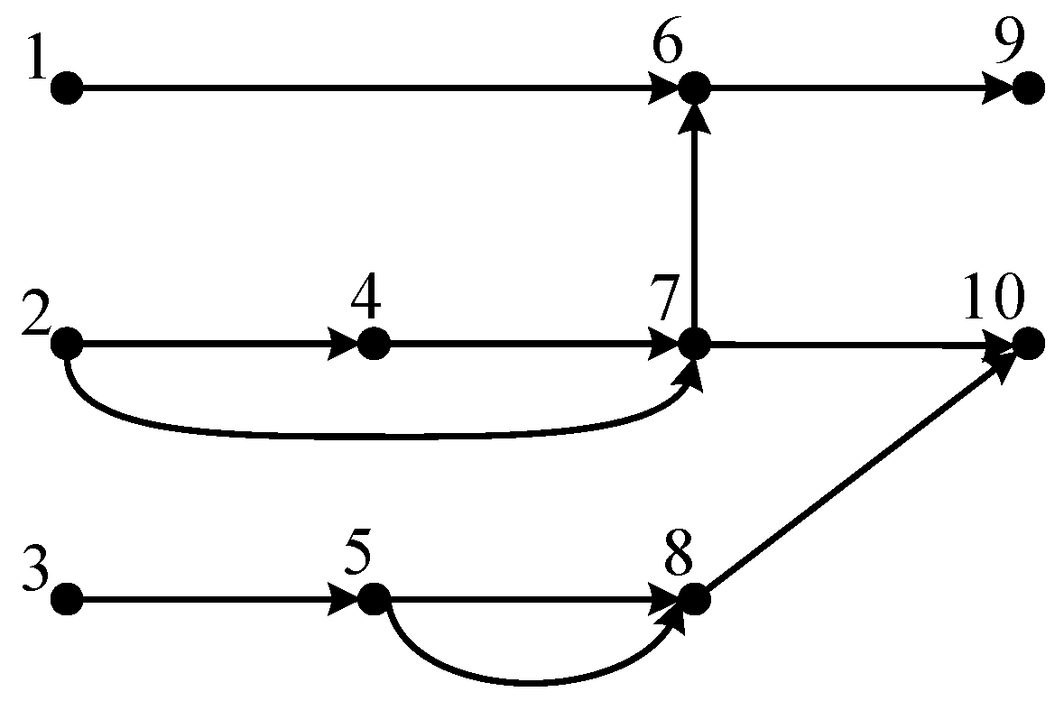
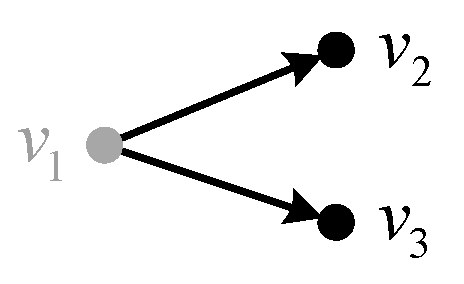
The corresponding E-matrix of the simple variable association diagram shown in Figure 5 can be derived as shown in Equation (2).

$$\mathrm{E}=\left[\begin{array}{cccc}0& 1& 0& 0\\ 0& 0& 1& 0\\ 0& 1& 0& 2\\ 0& 0& 0& 0\end{array}\right],$$

(2)

3.2. Analysis Method of the Influencing Factors and Influencing Paths of an Observed Variable

This paper introduces a path analysis methodology aimed at elucidating the relationships between specific variables. The variables in a system that need to be controlled and have an impact on the system are called control variables, denoted as $v^{\mathrm{c}}$. The variables in a system that need to be observed and can be observed are called observed variables, denoted as $v^{\mathrm{o}}$. Other variables that are directly or indirectly associated with control variables or observed variables are called transitional variables and are denoted as $v^{\mathrm{t}}$.

An observed variable may be influenced by multiple control variables in different ways. By tracing all paths terminating at a specific node, we can ascertain which control variables affect the observed variable corresponding to that node, as well as the possible paths of such an influence.

Assuming the j-th variable $v_j$ in the system is the observed variable, the element of the j-th column and i-th row in the E-matrix represents the number of causalities between $v_i$ to $v_j$. For each non-zero $e_{ij}$ found, the variable $v_i$ corresponding to the i-th row is recorded, and we simultaneously check whether the element $e_{ki}$ in the i-th column is zero. If a non-zero element is found, we continue to check further back in this manner, repeating the process until the row index of a non-zero element corresponds to a node number of a control variable.

The search process for the influencing factors and paths of an observed variable is illustrated in Figure 6.

In Figure 6, N represents the number of non-zero elements in the j-th column of the E-matrix, and the row indices of these non-zero elements are recorded in the set {list}.

For simple systems, the influencing factors of the observed variables can be directly inferred from the variable association diagram. For a system with a large number of variables and high dimensionality, it is difficult to see it directly from the variable association diagram, so the analysis shown in Figure 6 is required.

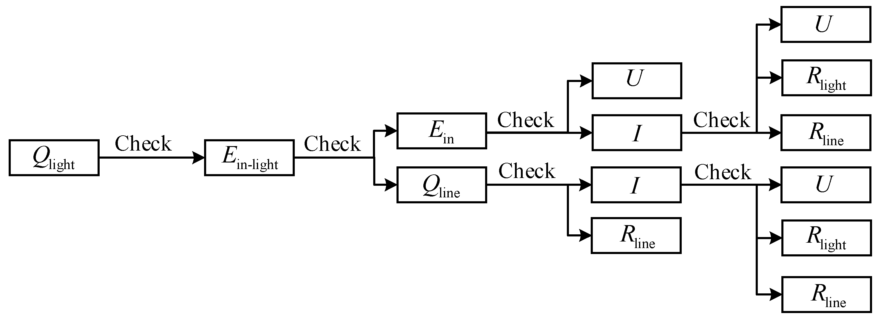
The building lighting system represented in Figure 4 can be taken as an example, demonstrating the search process for identifying the influencing factors of an observed variable. $Q_{\mathrm{light}}$ is the observed variable, and $U,R_{\mathrm{light}},R_{\mathrm{line}}$ are the control variables. We are searching for the influencing factors of $Q_{\mathrm{light}}$. Input the variable association matrix. The check module is applied to $Q_{\mathrm{light}}$, and the elements in column $Q_{\mathrm{light}}$ of the matrix that are not 0 correspond to $E_{\mathrm{in}-\mathrm{light}}$. The check module is continuously applied to $E_{\mathrm{in}-\mathrm{light}}$ until all variables found are control variables, and the serial number of the variables is recorded in the set Y. The process is shown in Figure 7.

3.3. Path Analysis Method of the Influence of a Control Variable

A control variable may influence multiple observed variables in different manners. By tracing all the paths originating from a specific node, we can ascertain which observed variables are influenced by the control variable corresponding to that node, as well as identifying the potential pathways of such an influence.

Assuming the i-th variable $v_i$ in the system is the control variable, the element of the i-th row and j-th column in the E-matrix represents the number of causalities between $v_i$ to $v_j$. For each non-zero $e_{ij}$ found, the variable $v_j$ corresponding to the j-th column is recorded, and we simultaneously check whether the element $e_{jk}$ in the j-th row is zero. If a non-zero element is found, we continue to check backward in this manner, repeating the process until the column index of a non-zero element corresponds to a node number of an observed variable. The specific search process is similar to that in Figure 5.

4. Quantitative Analysis Method of the Effects of Variables

4.1. Influence Mechanism between Variables

4.1.1. Influence between Any Two Variables

Each variable in the system can be written as a function of all variables, as shown in Equation (3).

$$\{\begin{array}{c}{v}_1=h_1(v_1,v_2,\dots ,v_n)\\ v_2=h_2(v_1,v_2,\dots ,v_n)\\ ⋮\\ v_n=h_n(v_1,v_2,\dots ,v_n)\end{array},$$

(3)

To precisely capture the specific interplay between two variables, we perform partial differentiation on Equation (3) and express the resulting derivatives in a matrix form, such as Equations (4) and (5).

$$\mathsf{\Delta }{\mathit{V}}^{\prime }=\mathit{J}\cdot \mathsf{\Delta }\mathit{V},$$

(4)

$$\left[\begin{array}{c}\mathsf{\Delta }{v}_1^{\prime }\\ \mathsf{\Delta }{v}_2^{\prime }\\ ⋮\\ \mathsf{\Delta }{v}_n^{\prime }\end{array}\right]=\left[\begin{array}{cccc}{J}_{11}& J_{12}& \cdots & J_{1n}\\ J_{21}& J_{22}& & ⋮\\ ⋮& & \ddots & \\ J_{n1}& \cdots & & J_{nn}\end{array}\right]\left[\begin{array}{c}\mathsf{\Delta }{v}_1\\ \mathsf{\Delta }{v}_2\\ ⋮\\ \mathsf{\Delta }{v}_n\end{array}\right],$$

(5)

where $\mathsf{\Delta }\mathit{V}$ represents the active change in variable V; $\mathsf{\Delta }{\mathit{V}}^{\prime }$ represents the actual change in variable V; Matrix J is the Jacobian matrix, herein, $J_{ij}={\displaystyle \raisebox{1ex}{$\partial v_i$}\!\left/ \!\raisebox{-1ex}{$\partial v_j$}\right.}$.

Many variables may not be correlated with each other, and those that are correlated may not interact equally, so the J-matrix tends to be an asymmetric sparse matrix with diagonal elements of one.

4.1.2. Influence of Control Variables on Observed Variables

In practical applications, more attention is paid to the influence of control variables on observed variables. Placing the control variables (assuming there are $n_{\mathrm{c}}$) on the right-hand side of the equation and the observed variables (assuming there are $n_{\mathrm{o}}$) on the left-hand side of the equation, the equations shown in Equations (6) and (7) are derived, which are used to characterize the effect of the control variables on the observed variables.

$$\mathsf{\Delta }{\mathit{V}}^{\mathrm{o}}=\mathit{F}\cdot \mathsf{\Delta }{\mathit{V}}^{\mathrm{c}},$$

(6)

$$\left[\begin{array}{c}\mathsf{\Delta }{v}_1^{\mathrm{o}}\\ \mathsf{\Delta }{v}_2^{\mathrm{o}}\\ ⋮\\ \mathsf{\Delta }{v}_{n_{\mathrm{o}}}^{\mathrm{o}}\end{array}\right]=\left[\begin{array}{cccc}{f}_{11}& f_{12}& \cdots & f_{1n_{\mathrm{c}}}\\ f_{21}& f_{22}& & ⋮\\ ⋮& & \ddots & \\ f_{n_{\mathrm{o}}1}& \cdots & & f_{n_{\mathrm{o}}{n}_{\mathrm{c}}}\end{array}\right]\left[\begin{array}{c}\mathsf{\Delta }{v}_1^{\mathrm{c}}\\ \mathsf{\Delta }{v}_2^{\mathrm{c}}\\ ⋮\\ \mathsf{\Delta }{v}_{n_{\mathrm{c}}}^{\mathrm{c}}\end{array}\right],$$

(7)

The matrix F describes the mapping between the amount of change in the control variable and the amount of change in the observed variable. $\left|f_{ji}\right|$ represents the influence intensity of the control variable on the observed variable. The larger the value of $\left|f_{ji}\right|$, the stronger the ability to affect the change in the control variable on the change in the observed variable.

4.2. Analysis of Two Typical Scenarios

4.2.1. Quantitative Analysis of an Observed Variable Affected by Multiple Control Variables

For a specified observed variable $v_j^{\mathrm{o}}$, when there are multiple paths connected to its corresponding node j, it means that it is affected by more than one control variable (assuming there are $n_{\mathrm{c}}$) at the same time, and its quantitative relationship is shown in Equation (8).

$$\mathsf{\Delta }{v}_j^{\mathrm{o}}={\displaystyle \sum _{i=1}^{n_{\mathrm{c}}}{f}_{ji}\mathsf{\Delta }{v}_i^{\mathrm{c}}=\left[f_{j1}{f}_{j2}\cdots f_{j{n}_{\mathrm{c}}}\right]\left[\begin{array}{c}\mathsf{\Delta }{v}_1^{\mathrm{c}}\\ \mathsf{\Delta }{v}_2^{\mathrm{c}}\\ ⋮\\ \mathsf{\Delta }{v}_{n_{\mathrm{c}}}^{\mathrm{c}}\end{array}\right]},$$

(8)

4.2.2. Quantitative Analysis of a Control Variable Affecting Multiple Observed Variables

For a specified control variable $v_i^{\mathrm{c}}$, when its corresponding node i has paths leading to different observed variables, it means that it can affect more than one observed variable at the same time (assuming there are $n_{\mathrm{o}}$), and its quantitative relationship is shown in Equation (9).

$$\left[\begin{array}{c}\mathsf{\Delta }{v}_1^{\mathrm{o}}\\ \mathsf{\Delta }{v}_2^{\mathrm{o}}\\ ⋮\\ \mathsf{\Delta }{v}_{n_{\mathrm{o}}}^{\mathrm{o}}\end{array}\right]=\left[\begin{array}{c}{f}_{1i}\\ f_{2i}\\ ⋮\\ f_{n_{\mathrm{o}}i}\end{array}\right]\cdot \mathsf{\Delta }{v}_i^{\mathrm{c}},$$

(9)

Two issues deserve attention:

(1)

Influence of a control variable on the whole system

A change in the control variable changes multiple observed variables affected by it, and results in an overall amount of change in the system:

$${\displaystyle \sum _{j=1}^{n_{\mathrm{o}}}\mathsf{\Delta }{v}_j^{\mathrm{o}}}=({\displaystyle \sum _{j=1}^{n_{\mathrm{o}}}{f}_{ji}})\mathsf{\Delta }{v}_i^{\mathrm{c}}=f_{\sum }\cdot \mathsf{\Delta }{v}_i^{\mathrm{c}},$$

(10)

If $f_{\sum }>0$, it signifies that the overall change in direction of the system aligns with the direction of change exhibited by the control variable; if $f_{\sum }<0$, it signifies that the overall change in direction of the system is contrary to the direction of change exhibited by the control variable.

(2)

Correlations between observed variables

Multiple observed variables $\left\{v^{\mathrm{o}}\right\}$ are simultaneously influenced by the control variable $v_i^{\mathrm{c}}$, and they exhibit correlation among themselves. Suppose that the two variables are $v_j^{\mathrm{o}}$ and $v_k^{\mathrm{o}}$. Compare $f_{ji}$ and $f_{ki}$ in the F-matrix. $v_j^{\mathrm{o}}$ and $v_k^{\mathrm{o}}$ are positively correlated when $f_{ji}$ and $f_{ki}$ are positive or negative at the same time. $v_j^{\mathrm{o}}$ and $v_k^{\mathrm{o}}$ are positively correlated. Conversely, when $f_{ji}$ and $f_{ki}$ have opposite signs, it indicates a negative correlation between $v_j^{\mathrm{o}}$ and $v_k^{\mathrm{o}}$.

There is a correlation between an observed variable $v_j^{\mathrm{o}}$ and all the observed variables as a whole $\left\{v^{\mathrm{o}}\right\}$ affected by the same control variable $v_i^{\mathrm{c}}$; its correlation coefficient is:

$${\beta }_j={\displaystyle \frac{{\displaystyle \sum \mathsf{\Delta }{v}_k^{\mathrm{o}}}}{\mathsf{\Delta }{v}_j^{\mathrm{o}}}}={\displaystyle \frac{f_{\sum }}{f_{ji}}},$$

(11)

If ${\beta }_j>0$, it indicates that the overall change trend in the observed variables $\left\{v^{\mathrm{o}}\right\}$ is the same as that of the control variable $v_j^{\mathrm{o}}$; if ${\beta }_j<0$, it indicates that the overall change trend in the $\left\{v^{\mathrm{o}}\right\}$ is the opposite to that of the $v_j^{\mathrm{o}}$.

Using the data-driven method to judge association rules requires the collection of a large amount of data and demands high data completeness and accuracy. With Equation (11), for a system whose principle is clear and the model is determined, the correlation coefficients between local variables and global variables can be determined by a limited number of sets of data.

5. Application of Variable Association in Energy Saving Fields

In actual energy usage scenarios, there is often not a single form of energy involved, and a multitude of losses may occur. These losses can be influenced by various factors, and correlations may exist among different types of losses. All these circumstances should be considered when formulating energy-saving measures.

5.1. Initial Selection of Energy-Saving Measures

The initial selection of energy-saving measures involves two primary considerations: determining which loss to target for energy saving, and identifying the specific influencing factor of that loss to address with measures.

(1)

Selection of maximum loss

If there are multiple losses in the system and the losses can be quantitatively compared (including approximate estimates and empirical perceptions), energy-saving measures are often prioritized for the largest loss. Because the amount of this loss is large, the corresponding energy-saving potential is naturally the largest. If technical measures for this loss are difficult or too costly, other losses can also be considered as targets for energy-saving measures.

(2)

Selection of the most significant influencing factor

According to the analysis in Section 4.2.1, a variable may be affected by multiple factors. Once a loss has been selected, it is crucial to observe its influencing factors, prioritize them based on their influence intensity, and then implement energy-saving measures targeting the factor with the highest influence intensity. This approach often leads to significant energy-saving results. Sometimes, although a certain factor has the greatest impact, if the energy-saving program based on that factor is difficult to implement or the cost is too high, energy conservation can also be carried out from other influence factors.

The following is an example of heat dissipation in a building. The main heat loss of a building consists of heat dissipation $Q_1$ from the walls and heat dissipation $Q_2$ from the windows [38]:

$$Q_1={\alpha }_1{A}_1\mathsf{\Delta }T,$$

$$Q_2={\alpha }_2{A}_2\mathsf{\Delta }T,$$

where ${\alpha }_1,{\alpha }_2$ denote the heat dissipation coefficients of the wall and window, respectively, $A_1,A_2$ denote the heat dissipation areas of the wall and window, respectively, and $\mathsf{\Delta }T$ denotes the indoor–outdoor temperature difference.

$Q_2$ accounts for a large portion of building heat dissipation [39], and it is generally considered first when energy-saving measures are developed.

Assume that the total heat dissipation area of the building is A and the area ratio of window to wall is k. The total building loss Q is:

$$Q=Q_1+Q_2=({\alpha }_1{\displaystyle \frac{A}{k+1}}+{\alpha }_2{\displaystyle \frac{kA}{k+1}})\mathsf{\Delta }T,$$

The wall heat dissipation coefficient is assumed to be constant. ${\alpha }_2$ and k are control variables, and Q is an observed variable. Equations in the form of Equation (7) are obtained:

$$\mathsf{\Delta }Q=\left[\begin{array}{cc}{f}_1& f_2\end{array}\right]\left[\begin{array}{c}\mathsf{\Delta }{\alpha }_2\\ \mathsf{\Delta }k\end{array}\right],$$

where $f_1={\displaystyle \frac{k}{k+1}}A\mathsf{\Delta }T$, $f_2={\displaystyle \frac{(2k+1){\alpha }_2+{\alpha }_1}{{(k+1)}^2}}A\mathsf{\Delta }T$. Compare the values of $\left|f_1\right|$ and $\left|f_2\right|$, under the condition that the two control variables change in the same amplitude. If $\left|f_1\right|$ is larger, the change in the heat dissipation coefficient ${\alpha }_2$ has a greater effect on the change in heat dissipated; if $\left|f_2\right|$ is larger, the change in k has a greater effect on the change in heat dissipated. If construction difficulty and cost are not taken into account, and the sole focus is on the energy-saving effect, then the choice of which control variable to target for energy-saving measures can be determined based on the relative magnitude of $\left|f_1\right|$ and $\left|f_2\right|$.

5.2. Additional Influence Analyses of Measures

According to the analysis in Section 4.2.2, a control variable may affect more than one loss. When changing the influence factor $v_i^{\mathrm{c}}$ with the goal of reducing loss $v_j^{\mathrm{o}}$, other losses may change as a result of the change in $v_i^{\mathrm{c}}$.

The following is an example of the electric heating system shown in Figure 8 to discuss the additional influences of energy-saving measures [40]. Herein, $R_1$ denotes the wire resistance and $R_2$ denotes the heating resistance.

System losses consist of two parts:

(1)

Loss on the wire resistance

$$P_1=I^2{R}_1={\left({\displaystyle \frac{U_1}{R_1+R_2}}\right)}^2{R}_1,$$

(2)

Loss on the heating resistance (equal to the heating power minus the effectively utilized power $P_0$)

$$P_2=I^2{R}_2-P_0={\displaystyle \frac{U_1^2{R}_2}{{(R_1+R_2)}^2}}-P_0,$$

Total system loss:

$$P_3=P_1+P_2,$$

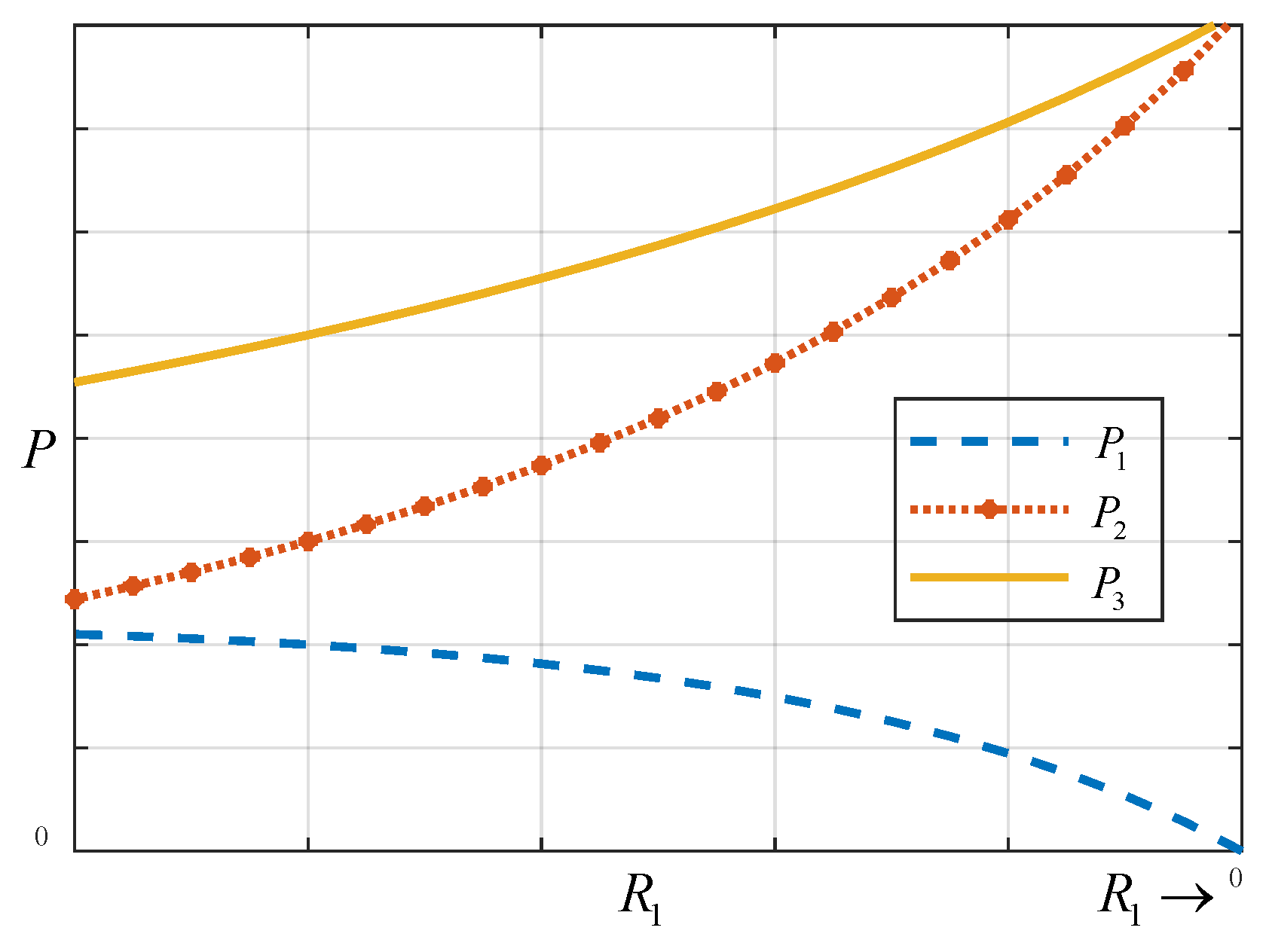
The variations in $P_1,P_2,P_3$ with $R_1$ are shown in Figure 9, where $R_1$ decreases as it shifts in the right direction.

Assuming that the voltage $U_1$ and resistance $R_2$ remain constant, $R_1$ can be reduced in order to reduce the wire resistance loss $P_1$. However, the reduction in $R_1$ increases the current I, which in turn increases the heating resistance loss $P_2$. As seen in Figure 9, with the decrease in $R_1$, although $P_1$ is reduced, $P_2$ and $P_3$ increase. In this case, to reduce $R_1$ is to reduce the wire resistance loss $P_1$, but an undesired result is given, that is, the total system loss increases instead.

5.3. Criteria of Effective Energy Saving

Effective energy-saving measures should meet the following requirements:

Requirement 1: The specific loss targeted by the measure can be reduced significantly (the energy saved is not less than the predetermined value $\mathsf{\Delta }{E}_0$), that is:

$$\{\begin{array}{l}\mathsf{\Delta }{v}_j^{\mathrm{o}}<0\hfill \\ \left|\mathsf{\Delta }{v}_j^{\mathrm{o}}\right|\ge \mathsf{\Delta }{E}_0\hfill \end{array},$$

(12)

Requirement 2: The sum of other losses will not increase significantly, that is:

$${\displaystyle \sum _{k\ne j}\mathsf{\Delta }{v}_k^{\mathrm{o}}}<\theta ,$$

(13)

where $\theta$ is a relatively small positive number, such as 1/10 of the predetermined energy saving value. When ${\displaystyle \sum _{k\ne j}\mathsf{\Delta }{v}_k^{\mathrm{o}}}<0$, it indicates that the sum of the other losses in the system decreases concurrently with the targeted loss being reduced by energy-saving measures; this represents the ideal scenario. Even if the other losses experience an increase, as long as this increase remains within permissible limits ($\theta$), effective energy savings for the system can still be achieved.

Substitute (9) and (10) into (12) and (13). Requirement 1 and requirement 2 may be described in terms of elements in the F-matrix as follows:

$$\{\begin{array}{l}\left|f_{ji}\right|\ge {\displaystyle \frac{\mathsf{\Delta }{E}_0}{\left|\mathsf{\Delta }{v}_i^{\mathrm{c}}\right|}}\hfill \\ f_{\sum }-f_{ji}>{\displaystyle \frac{\theta }{\mathsf{\Delta }{v}_i^{\mathrm{c}}}}\hfill \end{array},$$

(14)

Equation (14) can serve as a criterion for evaluating the effectiveness of energy-saving measures.

5.4. Scientific Processes for Formulating Energy-Saving Measures

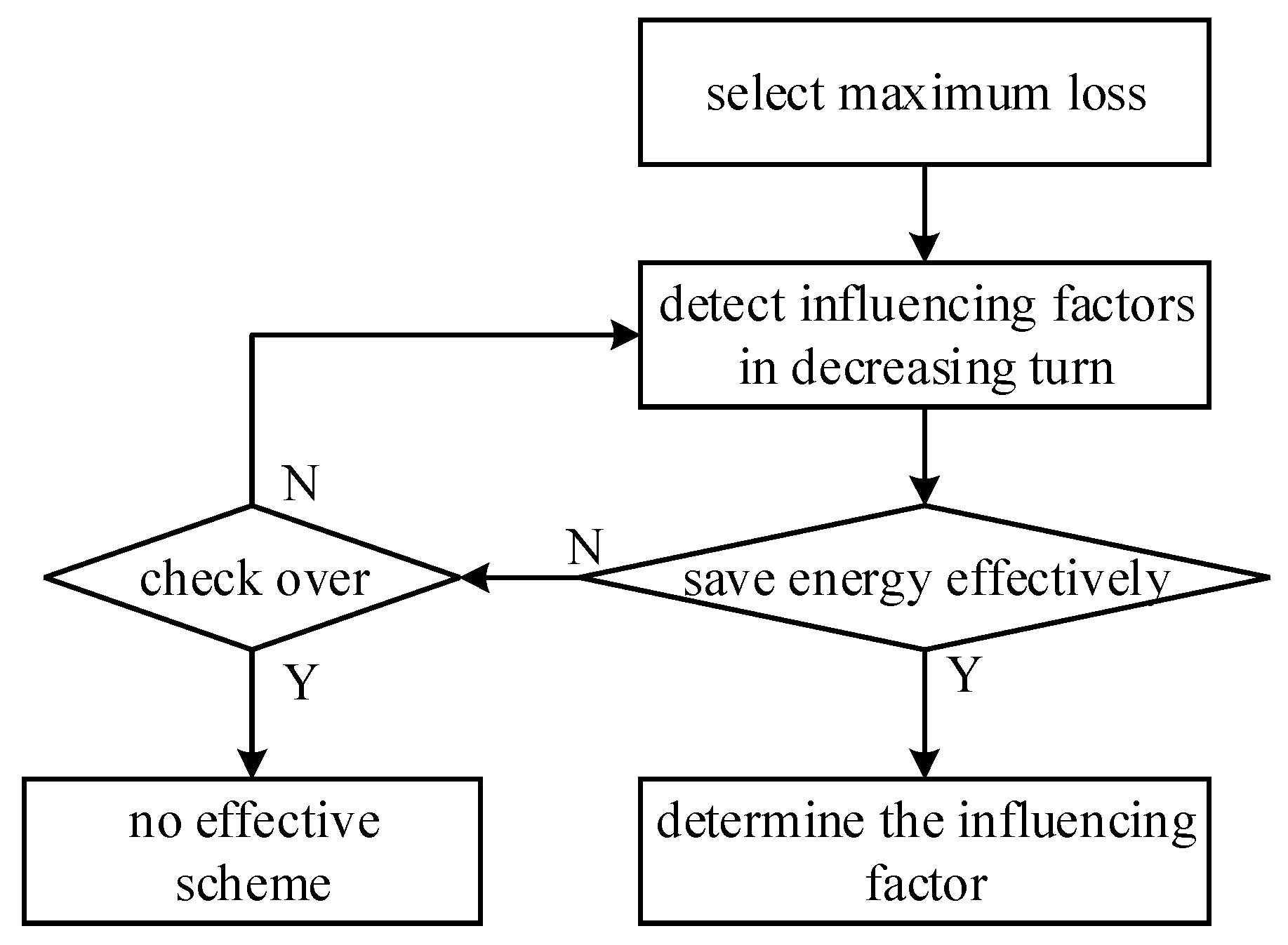
This paper proposes two schemes for formulating energy-saving measures.

(1)

A single energy-saving measure

Analyze the factors that influence $v_j^{\mathrm{o}}$ and rank them in descending order of their influence intensity. First, check whether the measure based on the factor with the highest influence intensity has an effective energy-saving ability, that is, whether it meets the criteria for effective energy saving. When satisfied, energy-saving measures are taken based on the influencing factor. Otherwise, the measure based on the factor with the second highest influence intensity should be considered, and it should be checked whether the criteria for effective energy saving is met. Continue this process until an influencing factor that meets the criteria is found. If none of the influencing factors related to $v_j^{\mathrm{o}}$ meet the criteria, it may not be advisable to implement energy-saving measures specifically for that loss. Instead, focus should be shifted towards energy-saving efforts for other losses.

The specific operation flow is shown in Figure 10.

(2)

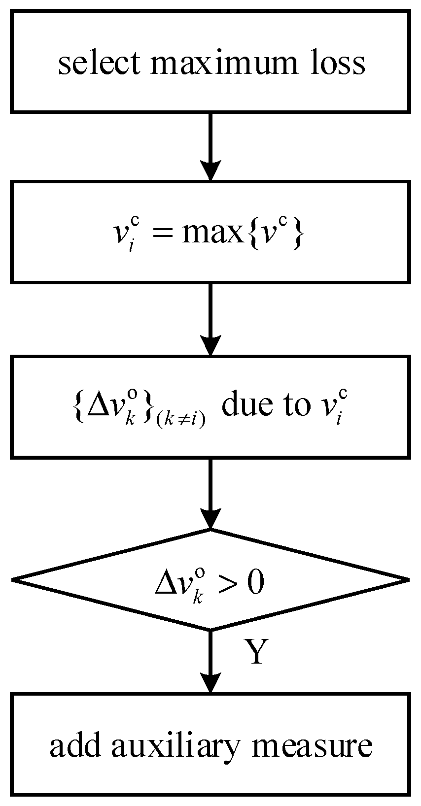
A combination of a main energy-saving measure and auxiliary measures

Among the influencing factors of $v_j^{\mathrm{o}}$, energy-saving measures should be formulated based on the factor $v_i^{\mathrm{c}}$ with the highest influence intensity. Assess the effect of $v_j^{\mathrm{o}}$ on other losses, and the set of other losses affected by $v_i^{\mathrm{c}}$ is denoted as $\left\{v_k^{\mathrm{o}}\right\}$, with the corresponding changes in those losses represented by $\left\{\mathsf{\Delta }{v}_k^{\mathrm{o}}\right\}$. Check whether the elements in $\left\{\mathsf{\Delta }{v}_k^{\mathrm{o}}\right\}$ are positive one by one. If an element is positive, then auxiliary measures based on other influencing factors of $v_i^{\mathrm{c}}$ need to be taken to ensure that this particular loss does not increase significantly. These auxiliary measures should be implemented alongside the energy-saving measures based on $v_i^{\mathrm{c}}$ to ensure effective overall energy savings.

The specific operation flow is shown in Figure 11. Herein, $\mathsf{\Delta }{v}_k^{\mathrm{o}}$ denotes the amount of loss variation.

Both schemes can ensure energy-saving effects, but they differ in the formulation and selection of measures, resulting in potentially varying degrees of energy savings. Generally speaking, the first scheme is simpler and easier to implement, making it the preferred choice for many enterprises. In contrast, the second scheme is slightly more complex, but it may leads to better energy-saving effects. Different industries and enterprises may choose different schemes according to their own actual situations.

5.5. Examples of Applications in Building Energy Savings

Consider the building lighting system (as shown in Figure 4). $U=230\mathrm{V},R_{\mathrm{line}}=0.013\mathsf{\Omega },R_{\mathrm{light}}=0.4\mathsf{\Omega }$, and $E_{\mathrm{light}}$ represents the effective energy required for the luminaire to emit the visible light of the specified illuminance, assumed to be 120,000 kWh. The energy consumption of the wire and luminaire are:

$$Q_{\mathrm{line}}={({\displaystyle \frac{U}{R_{\mathrm{line}}+R_{\mathrm{light}}}})}^2{R}_{\mathrm{line}}t,$$

$$Q_{\mathrm{light}}=E_{\mathrm{in}}-Q_{\mathrm{line}}-E_{\mathrm{light}},$$

$$E_{\mathrm{in}}=U{I}_{\mathrm{light}}t={\displaystyle \frac{U^2}{R_{\mathrm{line}}+R_{\mathrm{light}}}}t,$$

In order to reduce line loss $Q_{\mathrm{line}}$, the most intuitive energy saving idea is to reduce the wire resistance. Within a certain period (1000 h), if the line loss is expected to decrease by 3000 kWh, the resistance of the conductor needs to be reduced by 0.01$\mathsf{\Omega }$. It should be noted that changing $R_{\mathrm{line}}$ will not only affect $Q_{\mathrm{line}}$, but also $Q_{\mathrm{light}}$. When adopting this energy-saving measure, it is necessary to carefully examine its overall energy-saving effect.

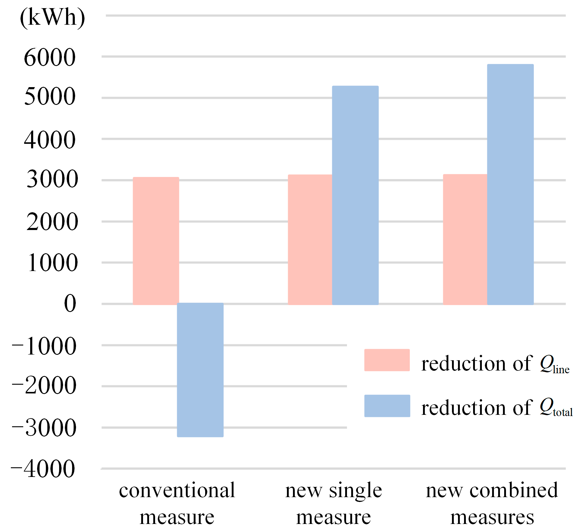
When taking energy-saving measures to reduce $R_{\mathrm{line}}$ from 0.013$\mathsf{\Omega }$ to 0.003$\mathsf{\Omega }$, $Q_{\mathrm{line}}$ decreases by 3054 kWh and $Q_{\mathrm{light}}$ increases by 6263 kWh. It is evident that this energy-saving measure not only fails to save energy, but also increases the system loss $Q_{\mathrm{total}}$ by 3209 kWh.

Now, try the energy saving idea proposed in this paper. Taking $Q_{\mathrm{line}}$ and $Q_{\mathrm{light}}$ as the observed variables, and U and $R_{\mathrm{line}}$ as the control variables, the equation for the effect of the control variables on the observed variables is:

$$\left[\begin{array}{c}\mathsf{\Delta }{Q}_{\mathrm{light}}\\ \mathsf{\Delta }{Q}_{\mathrm{line}}\end{array}\right]=\left[\begin{array}{cc}{f}_{11}& f_{12}\\ f_{21}& f_{22}\end{array}\right]\left[\begin{array}{c}\mathsf{\Delta }{R}_{\mathrm{line}}\\ \mathsf{\Delta }U\end{array}\right],$$

where

$$f_{11}={\left({\displaystyle \frac{U}{R_{\mathrm{line}}+R_{\mathrm{light}}}}\right)}^{2}t-{\displaystyle \frac{2R_{\mathrm{line}}{U}^{2}t}{{\left(R_{\mathrm{line}}+R_{\mathrm{light}}\right)}^3}},$$

$$f_{12}={\displaystyle \frac{2R_{\mathrm{line}}Ut}{{\left(R_{\mathrm{line}}+R_{\mathrm{light}}\right)}^2}},$$

$$f_{21}={\displaystyle \frac{2R_{\mathrm{line}}{U}^{2}t}{{\left(R_{\mathrm{line}}+R_{\mathrm{light}}\right)}^3}}-{\displaystyle \frac{2U^{2}t}{{\left(R_{\mathrm{line}}+R_{\mathrm{light}}\right)}^2}},$$

$$f_{22}={\displaystyle \frac{2Ut}{R_{\mathrm{line}}+R_{\mathrm{light}}}}-{\displaystyle \frac{2R_{\mathrm{line}}Ut}{{\left(R_{\mathrm{line}}+R_{\mathrm{light}}\right)}^2}},$$

Factors that influence $Q_{\mathrm{line}}$ include $R_{\mathrm{line}}$ and U. While reducing $R_{\mathrm{line}}$ can decrease $Q_{\mathrm{line}}$, it results in an increase in overall loss, failing to achieve the expected energy-saving effect. Reducing the other control variable U from 230 V to 228 V results in a decrease in $Q_{\mathrm{line}}$ by 3117 kWh, $Q_{\mathrm{light}}$ by 2148 kWh, and an overall loss in $Q_{\mathrm{total}}$ of 5265 kWh. Not only does the reduction in line loss reach the expected value of 3000 kWh, but the overall loss is significantly reduced as well. It is evident that the first energy-saving measure proposed in this paper facilitates the identification of effective energy-saving measures that meet the specified energy saving requirements.

Let us take a look at the second energy-saving measure. $R_{\mathrm{line}}$ is reduced from 0.013 to 0.003 $\mathsf{\Omega }$, which can be used as a major energy-saving measure to reduce $Q_{\mathrm{line}}$. The increase in $Q_{\mathrm{light}}$ is compensated by adjusting U. When the voltage drops from 230 V to 222 V, $Q_{\mathrm{line}}$ decreases by 3121 kWh, $Q_{\mathrm{light}}$ decreases by 2673 kWh, and the overall loss in $Q_{\mathrm{total}}$ decreases by 5794 kWh. It can be seen that the second energy-saving measure proposed in this paper can also achieve effective energy savings through the combination of primary and auxiliary measures.

A similar discussion can be made for other energy-using parts of the building.

Many enterprises tend to focus on addressing only one type of loss when formulating energy-saving measures, rarely considering the impact of these measures on other types of losses. This may result in the energy-saving effects of the measures failing to meet expectations. The two energy-saving measures proposed in this paper seem complex, but they fully consider the influence of system variables, and can effectively ensure the effect of energy-saving measures. Both ideas may achieve effective energy savings in the system.

A comparison of energy savings between target loss and overall loss among three energy saving ideas is shown in Figure 12.

6. Conclusions and Discussion

Within a relatively complex energy system, multiple losses frequently arise, each loss may be influenced by multiple factors, and a certain correlation may exist between these losses and influencing factors. Traditional energy-saving approaches tend to focus on a specific loss, and seldom consider the potential correlation and influence between multiple losses.

Unlike methods that rely heavily on data, such as regression analysis and Copula analysis, this paper proposes a variable correlation analysis method based on paths and correlation matrices from a principled perspective. It analyzes the influencing factors and impact paths of the observed variables and which observed variables are affected by a control variable.

We present a quantitative analysis method to assess the influence between variables, specifically emphasizing its application in energy saving. The initial selection of energy-saving measures should be based on the intensity of the factors influencing the target loss. When adopting an energy-saving measure, it is crucial to consider its additional impacts and to evaluate both the trend and the extent of its effect on the overall system loss.

Two schemes for formulating energy-saving measures are presented. The first scheme formulates energy-saving measures based on the factor with the most comprehensive effect, considering the influence intensity of various factors of the target loss, taking into account their effects on other losses. The second scheme directly formulates energy-saving measures based on the factor with the greatest influence on the target loss, and addresses any negative impacts on other losses through auxiliary measures.

The variable association analysis method proposed in this paper is a generalized method, which can not only help specific enterprises solve problems scientifically, but can also contribute to the formation of a general problem-solving mindset across various industries. In addition to its good application in the field of energy saving, it can also be widely used in the fields of construction, transportation, climate change, and so on. It is hoped that the achievements of this paper can make certain contributions to the areas of energy savings, emission reductions, and carbon reductions.

This paper is mainly applicable to systems with clear mathematical models, such as electric arc furnace steelmaking, building energy consumption, etc. The two proposed energy-saving measures have not yet been verified through extensive engineering practices and may still have some unconsidered details. Subsequent research should be conducted in greater depth, collaborating with professionals in related energy consumption fields to put relevant theories to the test in practice and continuously refine them.