Abstract
Accurate and reliable medium- and long-term load forecasting is crucial for the rational planning and operation of power systems. However, existing methods often struggle to accurately extract and capture long-term dependencies in load data, leading to poor predictive accuracy. Therefore, this paper proposes a medium- and long-term residential load forecasting method based on FEDformer, aiming to capture long-term temporal dependencies of load data in the frequency domain while considering factors such as electricity prices and temperature, ultimately improving the accuracy of medium- and long-term load forecasting. The proposed model employs Discrete Cosine Transform (DCT) for frequency domain transformation of time-series data to address the Gibbs phenomenon caused by the use of Discrete Fourier Transform (DFT) in FEDformer. Additionally, causal convolution and attention mechanisms are applied in the frequency domain to enhance the model’s capability to capture long-term dependencies. The model is evaluated using real-world load data from power systems, and experimental results demonstrate that the proposed model effectively learns the temporal and nonlinear characteristics of load data. Compared to other baseline models, DCTformer improves prediction accuracy by 37.5% in terms of MSE, 26.9% in terms of MAE, and 26.24% in terms of RMSE.
1. Introduction
Residential load forecasting plays a crucial role in the planning and design of residential area power systems, aiming to ensure their safe, economical, and reliable operation; meet electricity demands; and promote sustainable development in residential areas. With the continuous progress of urbanization, electricity consumption has surged. However, the uneven distribution of social energy resources has led to the issue of load imbalance in residential district power grids. Therefore, accurate and rational residential load forecasting is essential in guiding the planning of residential district facilities [1]. Simultaneously, in-depth research into residential loads helps in formulating demand-side management policies, such as peak-time tariffs and energy reserves, thereby guiding residents to reduce electricity consumption during peak hours and balance the load.
Presently, load forecasting primarily falls under two categories: traditional forecasting methods and machine learning-based forecasting methods. Traditional approaches encompass the single consumption method, the trend analysis method [2], and the load density method [3], among others. Meanwhile, machine learning-based methods include Convolutional Neural Networks (CNNs) [4], Long Short-Term Memory (LSTM) [2,5], General Regression Neural Networks (GRNNs) [6], and the like. Nonetheless, these methods encounter limitations, including the subpar accuracy of long time series load prediction, shallow analysis of influencing factors, and the challenge of adapting to the rapid changes in, and diverse development of, residential areas.
To improve the accuracy of long-term prediction, some researchers have introduced an attention mechanism. This mechanism focuses on important information, disregards less significant data with low weights, and continually adjusts weights. Thus, the model can select crucial information even in varying scenarios, thereby enhancing load forecasting accuracy [7,8,9]. The authors of [10] proposed a neural network based on Long Short-Term Memory (LSTM) for mid-term load forecasting. Although LSTM achieves higher accuracy in short-term load forecasting, it fails to capture long-term temporal features. Consequently, references [11,12] improved upon LSTM by incorporating attention mechanisms, introducing the Attention-LSTM model, which achieved better long-term prediction performance but still could not fundamentally address the issue of LSTM’s gradient explosion. The authors of [13] introduced a novel sequence modeling paradigm: Transformer. The emergence of the Transformer has led to breakthroughs in long sequence tasks. The self-attention mechanism in the Transformer model allows the model to directly attend to information from other positions in the sequence, thus performing better in capturing long-distance dependencies and resolving the poor parallel computing capabilities caused by sequence dependencies in Recurrent Neural Networks (RNNs). References [14,15,16] applied Transformer and its variant models to the field of load forecasting, achieving significant improvements in both short-term and long-term prediction aspects. In recent years, an increasing number of Transformer variant models have been proposed. For instance, the authors of [17] improved upon the Transformer by introducing Convolutional Self-Attention and the LogSparse Transformer. By incorporating causal convolutions to enhance the model’s ability to focus on context, training speed was increased. The authors of [18] proposed the FEDformer model, based on the Transformer model. By using Discrete Fourier Transform (DFT) and wavelet transform to convert temporal information into frequency domain information, prediction accuracy and time complexity were further improved, although the potential for Gibbs problems to arise was noted.
Therefore, existing load forecasting still faces several challenges. Traditional forecasting methods typically rely on statistical features and regularities in historical data, but they are limited when confronted with complex load variations and external influencing factors. They often struggle to accurately capture long-term temporal dependencies, resulting in poor accuracy in long-term load forecasting. On the other hand, deep learning-based methods have made some progress with the introduction of attention mechanisms, yet they still fail to capture the complex dependencies present in long-term time series.
In summary, to address the issues of traditional electricity load forecasting models being unable to accurately model long-term temporal dependencies and relying solely on historical load data, this paper proposes a load forecasting model based on DCTformer to achieve medium- and long-term load forecasting for residential areas. This paper proposes the DCTformer model, addressing the Gibbs phenomenon in FEDformer, which enhances the accuracy of long-term load forecasting. The method is empirically analyzed and compared with the predictions of the Informer model, FEDformer model, LSTM model, and Transformer model to validate its effectiveness and superiority.
The contributions of our work can be summarized as follows:
- This study goes beyond solely relying on historical load data for load forecasting by incorporating electricity prices and temperature information. This holistic approach provides a comprehensive and accurate foundation for load forecasting, enhancing the model’s grasp of load variations and thus improving forecasting accuracy.
- The DCTformer model is proposed, replacing the Discrete Fourier Transform in the FEDformer model with Discrete Cosine Transform, effectively eliminating the Gibbs effect and enhancing model stability.
- Additionally, a DCT attention mechanism is developed, which involves transforming load data into the frequency domain using Discrete Cosine Transform and introducing causal convolution, further improving prediction accuracy.
Additionally, this article is divided into five sections. Section 1 introduces the importance of accurate and reliable load forecasting in integrated power systems. Section 2 presents the background and methodology. Section 3 describes the method proposed in this article. Section 4, we present, analyze, and discuss the experimental results. Section 5 summarizes the work of the entire paper.
2. Background Theories
2.1. FEDformer Model
The FEDformer model was proposed by researchers from the Decision Intelligence Lab of Alibaba Dharmo Academy. It combines the advantages of the Transformer model with Periodic Trend Decomposition, innovatively utilizing the Fourier Transform to convert data from the time domain to the frequency domain. Within this domain, the data undergoes processing, and subsequently, a frequency domain-augmented attention mechanism is introduced to enhance prediction accuracy and efficiency. The FEDformer model, depicted in Figure 1 [17], primarily consists of a frequency enhancement module, a hybrid trend decomposition module, and a frequency enhancement attention module.
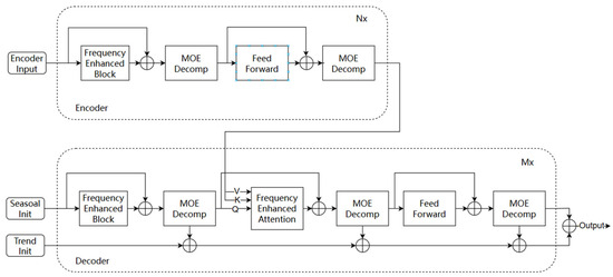
Figure 1.
The architecture of FEDformer [17].
Frequency Enhancement Module: The DFT is employed to convert input data into frequency-domain data via Fourier transformation. Subsequently, a random selection operation is conducted on the frequency domain, followed by the random initialization of matrix R, which is then multiplied with the randomly selected frequency components. To facilitate subsequent Fourier inverse transformation, it is necessary to zero-pad the data dimensions. Additionally, the frequency-domain data are converted back to time-domain data through Fourier inverse transformation.
where is the input data, is the DFT, and is the random selection operation.
Hybrid Trend Decomposition Module: We can overcome the problem of insufficient feature extraction by using the hybrid trend decomposition module with fixed-size windows in realistic situations with complex period and trend components. This mainly involves a number of windows of different sizes and can lead to the extraction of a number of different component features, which the authors have set weights for them, aiming to distinguish the contribution of different component features to the model. Finally, a weighted summation of the final trend data can be obtained by weighted summing.
Frequency-Enhanced Attention Module: This module replaces the conventional attention mechanism module, where and are obtained from the encoder through the multilayer perceptron, and is obtained from the decoder through the multilayer perceptron; are converted from time-domain data into frequency-domain data under the Fast Fourier Transform (FFT), and then they are randomly selected as components. The subsequent operations are the same as those of the conventional attention mechanism.
where is the query matrix, is the attention content, is the value, computes the attention weight on for , is the dimension of the matrix for the normalized attention mechanism, and is the normalized exponential function.
2.2. Discrete Cosine Transform
Discrete Cosine Transform (DCT) is a transformation method that converts a discrete sequence or signal into a set of discrete cosine functions. It finds extensive application in signal processing, image compression, audio processing, and various other fields.
DCT represents an input discrete sequence or signal as a linear combination of a set of orthogonal discrete cosine functions with different frequencies and amplitudes [19]. By performing an inner product operation of the input sequence with these cosine functions, a set of coefficients representing the energy of different frequency components of the input signal can be obtained. Commonly used DCT methods include DCT-I, DCT-II, DCT-III, and DCT-IV. Among these, DCT-II, also known as standard DCT, is the most commonly utilized form. In image and audio processing, DCT-II is frequently employed to convert signals into frequency-domain representations.
DCT finds wide applications in image and audio compression. In image compression, it is utilized in the Discrete Cosine Transform step of the JPEG compression algorithm to convert images into frequency-domain representations for compression. Similarly, in audio compression, DCT is extensively used in the transform step in audio coding standards such as MP3 and AAC.
DCT has also demonstrated excellence in the realm of time series prediction. Through DCT transformation, time-series data can be converted into the frequency domain, facilitating operations such as dimensionality reduction, compression, and feature extraction. DCT transformation can be regarded as a type of DFT where the input signal is a real-even function. Unlike DFT, which exhibits discontinuities at boundaries, leading to a large number of high-frequency contents and the Gibbs phenomenon, DCT [20] boasts symmetric scalability. This characteristic fundamentally mitigates the Gibbs effect and eliminates a significant amount of high-frequency artificial noise, rendering DCT more energy-efficient than DFT.
2.3. Causal Convolution
Causal convolution is a convolution operation used for processing temporal data, widely applied in deep learning tasks such as audio processing, speech recognition, and natural language processing.
In traditional convolution operations, the input data undergo sliding window operations, and the output is obtained by computing the product and summation operations between the convolution kernel and the data within the window. However, this convolutional operation lacks causality because each output time step may depend on future portions of the input data.
Causal convolution [21] addresses this issue by imposing a causal constraint. In causal convolution, the convolution kernel can only access data from the current time step. This ensures that each output time step solely relies on past information, thereby preserving causality.
Various techniques can be employed to implement causal convolution, such as padding in the convolution operation to restrict the convolution kernel to access only current and past data, or utilizing specially designed convolution kernel structures like the causal convolution kernel.
Maintaining causality, causal convolution proves particularly suitable for deep learning tasks involving temporal data, effectively capturing temporal information and enhancing model performance. Its structure diagram shows that the input sequence unfolds over time, with the convolutional kernel sliding along the time axis. Each convolution operation depends only on the current and past input information, generating the output sequence. This design ensures that the model does not leak future information during prediction, effectively addressing the causal relationship requirements in time series forecasting tasks. The process of causal convolution is illustrated in Figure 2.
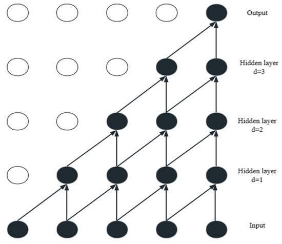
Figure 2.
The architecture of causal convolution.
3. Methodology
In this section, we will introduce (1) the overall structure of the DCTformer, as shown in Figure 3; (2) the DCT module and DCT attention module proposed in this paper; and (3) the training process of the model.
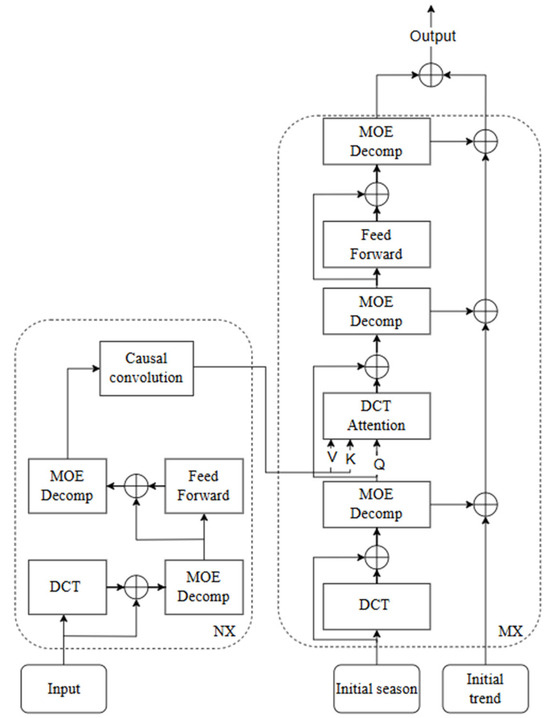
Figure 3.
The architecture of DCTformer.
Preliminary: The electricity load data are time-series data with multiple dimensions. We use to represent the length of the input load data and to represent the input dimension. Therefore, the input of the encoder is a matrix.
DCTformer Structure: As mentioned earlier, it is understood that DFT might lead to the Gibbs phenomenon. Therefore, building upon the FEDformer structure, we introduce the DCT module (DCT) and simultaneously enhance the attention mechanism, proposing the DCT attention mechanism (DCTAttention). Detailed explanations of DCT and DCTAttention will be provided in Section 2.2 and Section 2.3, respectively.
In designing the encoder, we drew inspiration from the classic transformer architecture and employed a multilayered encoder design to achieve better performance through stacking multiple layers. , represents the output of the -layer encoder. The historical input of electricity load data is denoted as . The formalization of the is as follows:
where denotes the seasonal component of the -layer decoder after the first decomposition, denotes the seasonal component of the -layer decoder after the second decomposition, denotes the input of the previous layer, and the DCT module is realized by the DCT, which ultimately yields the -layer output of the decoder, .
The decoder, like the encoder, also utilizes a multilayer structural design.
where , , represent the seasonal and trend components of the -th level 3 decomposition, respectively. DCTAttention is the DCT attention module, and is the projection of the th trend .
3.1. DCT Module
DCT has symmetric scalability, fundamentally avoids the Gibbs effect, and eliminates a lot of high-frequency artificial noise, making DCT more efficient than DFT.
In this module, we propose to replace DFT with DCT to realize the conversion operation, i.e., conversion from the time domain to the frequency domain.
The specific steps are as follows:
Step 1: input data are passed through the multilayer perceptron to increase nonlinearity.
Step 2: the data are transformed from being time-domain data to frequency-domain data by DCT transformation.
Step 3: we randomly select components for the frequency-domain data to improve the operation efficiency while retaining most of the information.
where is the output of the input data after the multilayer perceptron, is the DCT, and is the random selection operation.
Step 4: randomize the initial matrix R and multiply it with the randomly selected components from the previous step.
Step 5: after complementing the dimensions, use DCT inverse transformation to convert the frequency-domain data into time-domain data.
3.2. DCT Attention Mechanisms
In this module, the regular attention mechanism is also replaced with DCTAttention, whereby feature extraction is conducted under the frequency domain for q, k, v, and then, the computation of attention scores is performed. The specific steps are as follows:
Step 1: obtain and after multilayer perceptron and causal convolution in Encoder, and obtain after multilayer perceptron by Decoder.
Step 2: perform DCT transformation on the obtained to convert it to frequency-domain data, and then select the components randomly.
Step 3: perform the computation of attention scores in the frequency domain.
Step 4: randomize the initial matrix R and multiply it with the randomly selected components from the previous step.
Step 5: after complementing the dimensions, use DCT inverse transformation to convert the frequency-domain data into time-domain data.
3.3. Process Design
The specific implementation process is shown in Figure 4. Firstly, the load data are preprocessed and divided into a training set and a test set, and then the DCTformer model is constructed, and the loss function adopts Mean Square Error (MSE). Finally, the trained DCTformer model is saved, and the test set is used to verify the effectiveness of the model, and by analyzing the load prediction results, the shortcomings are found, and the prediction model is continuously optimized.
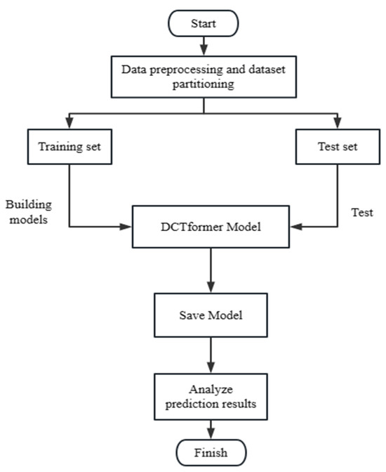
Figure 4.
Flowchart of DCTformer process.
4. Case Study
4.1. Dataset
To validate the performance of the DCTformer model proposed in this paper, a region’s real electricity load data, spanning from 1 January 2006 to 1 January 2011, were selected. The dataset comprises measurements taken at 30 min intervals, with units in MW. Additionally, the dataset includes variables such as humidity, temperature, tariff, and load data.
For training purposes, the dataset was partitioned into a training and testing set in a 7:3 ratio. The distribution of the dataset is shown in Figure 5.
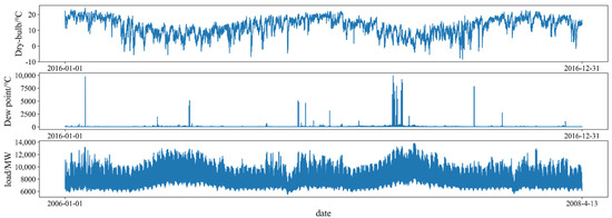
Figure 5.
Data display.
4.2. Evaluation Metrics
In this paper, Mean Square Error (MSE), RMSE, and Mean Absolute Error (MAE) are utilized as evaluation metrics for assessing the performance of the DCTformer model. Smaller values of MSE, RMSE, and MAE indicate more accurate model predictions. The formulas for calculating these metrics are provided below.
where denotes the true value, and denotes the predicted value. denotes the total number of test samples.
4.3. Gibbs Utility Experiment
In order to verify that DCT can solve the Gibbs effect caused by DFT when performing frequency domain transformation, the first 1000 data of the dataset were selected for the experiment. The extracted data were filtered by DCT and DFT, respectively, and compared with the original data, and the results are shown in Figure 6.
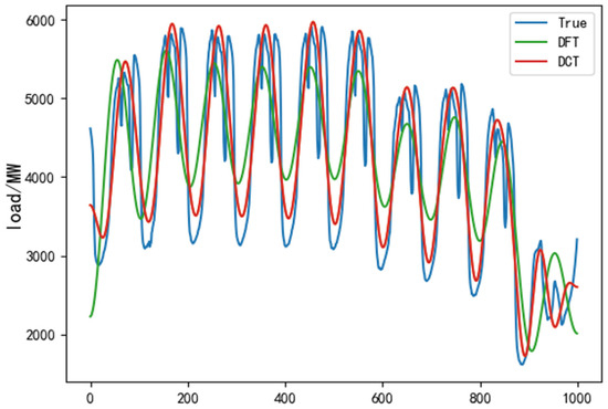
Figure 6.
Filter comparison chart.
In Figure 6, the blue color represents the original data, the red color represents the result of DCT filtering reconstruction, and the green color represents the result of DFT filtering reconstruction. From Figure 6, it can be seen that the result of DFT has serious distortion at both ends, which will have a greater impact on the next step of analysis and prediction, which is also known as Gibbs utility caused by DFT. In contrast, the reconstructed results after DCT filtering are basically consistent with the trend in the original data. This shows that DCT filtering can effectively solve the DFT generated when the Gibbs effect problem takes place.
4.4. Data Normalization
The normalization process serves several functions, including increasing the convergence speed of the model, improving its stability, and enhancing its generalization ability. However, during the actual load forecasting process, the model’s input typically encompasses various data with differing magnitudes. Normalizing the data aids in expediting model convergence, rectifying feature imbalances, and enhancing prediction stability and consistency. Hence, the input data are normalized as a preliminary step. In this paper, min–max normalization is employed to scale the data to the range of [0,1], with the calculation process outlined below.
where is the original measured data of the ith sampling point, is the value after the normalization of , and and are the maximum and minimum values of the data. When the normalized predicted value is obtained by inputting the data into the model using the normalized data from the above equation, it is then back-normalized using Equation (4).
where is the normalized conforming forecast value; is the actual electric load forecast value obtained after inverse normalization.
4.5. Hyperparameter Settings
In this paper, the DCTformer model is employed to realize medium- and long-term load forecasting within the park. The hyperparameter settings of the model significantly influence the forecasting results. These hyperparameters mainly include the number of iterative training times (epochs), batch size (batch_size), and learning rate (learning_rate), which are set to epochs = 100, batch_size = 64, and learning_rate = 0.001, respectively. Additionally, the number of layers for causal convolution can be selected based on data complexity. Through experimentation, this paper determines that the optimal number of layers for causal convolution is three.
To underscore the advantages of the proposed model, this paper introduces the following comparison algorithm models: the Informer model, LSTM model, Linear model, and Transformer model. To enhance experimental credibility, an equal number of iterations for training were set across all models.
4.6. Results and Discussion
To verify the accuracy and effectiveness of the proposed approach, load forecasting was conducted on the same dataset using Transformer, Fedformer, Informer, LSTM, and DCTFormer, with forecasting durations of 48 h, 168 h, and 360 h, respectively. The quantitative results of each model for the 48 h forecast duration are presented in Table 1.

Table 1.
Forecasting results (48 h), bold indicates the best result.
From Table 1, it is evident that the DCTFormer model proposed in this paper demonstrates superior performance on the test dataset, outperforming the Informer, Transformer, and LSTM models in both MSE and MAE evaluation metrics. This can be attributed to the superior learning capability of the DCTformer model, enabling it to effectively capture and fit the underlying features within the data. These results further validate the effectiveness and superiority of the DCTformer model proposed in this paper.
In order to verify the validity and accuracy of DCTformer in long-term forecasting, this paper continues with load forecasting with forecast lengths of 168 and 360 h, and the results are shown in Table 2 and Table 3.

Table 2.
Forecasting results (168 h), bold indicates the best result.

Table 3.
Forecasting results (360 h), bold indicates the best result.
Based on the prediction results in Table 2 and Table 3, in terms of 168 h load forecasting, the model proposed in this paper outperforms the comparative models in terms of MAE, MSE, and RMSE. In terms of 360 h load forecasting, the model proposed in this paper performs better than other models in terms of MAE and RMSE, with only slightly lower accuracy compared to the Transformer model in terms of MSE. Overall, the DCTformer model demonstrates superior fitting compared to the other comparative models. This is attributed to the processing of data in the frequency domain through DCT, which not only resolves the Gibbs problem but also enhances the model’s ability to capture global features of the time series. Combined with seasonal trend decomposition and causal convolution, the DCTformer model effectively retains earlier information and improves long-term forecast accuracy, a capability not observed in other comparative models.
Figure 7 displays the predicted curves of each model over a duration of 168 h. From Figure 7, it is evident that at peak load, other comparative models exhibit significant deviations, whereas the model proposed in this study aligns closely at peak times, demonstrating superior prediction stability and accuracy compared to other models. This superiority is attributed to the suitability of DCT for handling frequency-domain representations. In contrast, DFT may induce the Gibbs phenomenon when dealing with frequency-domain representations, resulting in blurry or distorted frequency information. By leveraging DCT, accurate representation of the frequency-domain characteristics of the input sequence is achieved, thereby enhancing the model’s understanding of time-series data and improving its accuracy, particularly during load peaks.
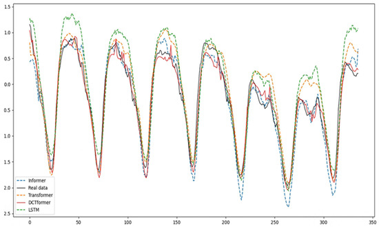
Figure 7.
Model prediction results.
Moreover, the exceptional performance of the model in long-term load forecasting tests is credited to the DCT attention mechanism proposed herein. DCT is employed to transform load data into the frequency domain for attention calculation, while causal convolution addresses potential information leakage in long-term load forecasting. The combination of causal convolution with the DCT attention mechanism optimizes model parameterization, enabling better adaptation to dynamic changes in input sequences, thereby reducing overfitting and enhancing generalization across different datasets.
Upon analysis of the quantitative results from Table 1, Table 2 and Table 3, alongside the prediction curves in Figure 7, it can be concluded that the proposed prediction model exhibits robustness and superior prediction accuracy. Additionally, to validate the model’s generalizability, an additional dataset, Electricity, was incorporated into the study. This dataset further evaluates the model’s performance and robustness across diverse scenarios, with experimental results detailed in Table 4. The prediction horizon was set to 360 h, and the evaluation metrics included MSE, MAE, and RMSE.

Table 4.
Forecasting results (360 h), bold indicates the best result.
Electricity is a classic, public time-series dataset commonly used for various time-series prediction tasks. This dataset was selected to further validate the generalizability of the model. As shown in Table 4 above, the proposed DCTformer model achieved state-of-the-art performance across all three evaluation metrics. This is likely because the model proposed in this paper has strong feature extraction capabilities, enabling it to capture key information in time-series data and thus perform well on time-series datasets from different domains.
5. Conclusions
This paper proposes a novel DCTformer model for electricity load forecasting. To address the Gibbs phenomenon caused by DFT in FEDformer, DCT is used for frequency domain transformation. Experiments on the Gibbs phenomenon demonstrate that using DCT for frequency-domain representations effectively reduces Gibbs artifacts, thereby improving prediction accuracy by minimizing spurious effects in the forecast results. To solve the problem of traditional models failing to capture long-term dependencies, the DCT attention mechanism is introduced. By applying multi-head attention mechanisms and causal convolution in the frequency domain, the model effectively captures long-term dependencies in time-series data. Additionally, considering the interdependence among dimensions in multivariate time series, the model integrates information such as temperature and electricity prices, further enhancing prediction accuracy. Experimental results show that the model can more accurately capture load fluctuations and changes and learn long-term dependencies in load data. Compared to other baseline models, DCTformer improves MSE by 37.5%, MAE by 26.9%, and RMSE by 26.24%.
Future research will consider load forecasting in more complex environments while enhancing the model’s ability to fit data through multi-model cross-learning [23].
Author Contributions
Validation, D.F. and Z.C.; Resources, D.L.; Writing—original draft, Q.L. All authors have read and agreed to the published version of the manuscript.
Funding
This work was supported by the Research and Development Project of Key Core and Common Technology of Shanxi Province (2020XXX007) and the Key Research and Development Projects of Shanxi Province (202102020101006).
Data Availability Statement
Data is contained within the article.
Conflicts of Interest
The authors declare no conflict of interest.
Abbreviations
The following abbreviations are used in this manuscript:
| CNN | Convolutional Neural Networks |
| CL | Cross-learning |
| DFT | Discrete Fourier Transform |
| DCT | Discrete Cosine Transform |
| LSTM | Long Short-Term Memory |
| GRNN | General Regression Neural Network |
| MSE | Mean Square Error |
| MAE | Mean Absolute Error |
| RMSE | Root Mean Square Error |
| RNNs | Recurrent Neural Networks (RNNs) |
References
- Aslam, S.; Herodotou, H.; Mohsin, S.M.; Javaid, N.; Ashraf, N.; Aslam, S. A survey on deep learning methods for power load and renewable energy forecasting in smart microgrids. Renew. Sustain. Energy Rev. 2021, 144, 110992. [Google Scholar] [CrossRef]
- Alhussein, M.; Aurangzeb, K.; Haider, S.I. Hybrid CNN-LSTM model for short-term individual household load forecasting. IEEE Access 2020, 8, 180544–180557. [Google Scholar] [CrossRef]
- Soliman, S.A.; Al-Kandari, A.M. Electrical Load Forecasting: Modeling and Model Construction; Elsevier: Amsterdam, The Netherlands, 2010. [Google Scholar]
- Liu, Y.; Wang, W.; Ghadimi, N. Electricity load forecasting by an improved forecast engine for building level consumers. Energy 2017, 139, 18–30. [Google Scholar] [CrossRef]
- Alghamdi, M.A.; Abdullah, S.; Ragab, M. Predicting Energy Consumption Using Stacked LSTM Snapshot Ensemble. Big Data Min. Anal. 2024, 7, 247–270. [Google Scholar] [CrossRef]
- Greff, K.; Srivastava, R.K.; Koutník, J.; Steunebrink, B.R.; Schmidhuber, J. LSTM: A search space odyssey. IEEE Trans. Neural Netw. Learn. Syst. 2016, 28, 2222–2232. [Google Scholar] [CrossRef] [PubMed]
- Wang, K.; Huang, S.B.; Ding, Y.L. Application of GRNN neural network in short term load forecasting. Adv. Mater. Res. 2014, 971, 2242–2247. [Google Scholar] [CrossRef]
- Wu, K.; Wu, J.; Feng, L.; Yang, B.; Liang, R.; Yang, S.; Zhao, R. An attention-based CNN-LSTM-BiLSTM model for short-term electric load forecasting in integrated energy system. Int. Trans. Electr. Energy Syst. 2021, 31, e12637. [Google Scholar] [CrossRef]
- Bohara, B.; Fernandez, R.I.; Gollapudi, V.; Li, X. Short-term aggregated residential load forecasting using BiLSTM and CNN-BiLSTM. In Proceedings of the 2022 International Conference on Innovation and Intelligence for Informatics, Computing, and Technologies (3ICT), Sakheer, Bahrain, 20–21 November 2022; pp. 37–43. [Google Scholar]
- Bouktif, S.; Fiaz, A.; Ouni, A.; Serhani, M.A. Optimal deep learning lstm model for electric load forecasting using feature selection and genetic algorithm: Comparison with machine learning approaches. Energies 2018, 11, 1636. [Google Scholar] [CrossRef]
- Qin, J.; Zhang, Y.; Fan, S.; Hu, X.; Huang, Y.; Lu, Z.; Liu, Y. Multi-task short-term reactive and active load forecasting method based on attention-LSTM model. Int. J. Electr. Power Energy Syst. 2022, 135, 107517. [Google Scholar] [CrossRef]
- Dai, Y.; Zhou, Q.; Leng, M.; Yang, X.; Wang, Y. Improving the Bi-LSTM model with XGBoost and attention mechanism: A combined approach for short-term power load prediction. Appl. Soft Comput. 2022, 130, 109632. [Google Scholar] [CrossRef]
- Wang, C.; Wang, Y.; Ding, Z.; Zheng, T.; Hu, J.; Zhang, K. A transformer-based method of multienergy load forecasting in integrated energy system. IEEE Trans. Smart Grid 2022, 13, 2703–2714. [Google Scholar] [CrossRef]
- Xing, Z.; Pan, Y.; Yang, Y.; Yuan, X.; Liang, Y.; Huang, Z. Transfer learning integrating similarity analysis for short-term and long-term building energy consumption prediction. Appl. Energy 2024, 365, 123276. [Google Scholar] [CrossRef]
- Jin, X.; Xuan, Y.; Zhou, X.; Chen, W.; Wang, Y.X.; Yan, X. Enhancing the locality and breaking the memory bottleneck of Transformer on time series forecasting. Adv. Neural Inf. Process. Syst. 2019, 32, 5243–5253. [Google Scholar]
- Liu, F.; Fu, Z.; Wang, Y.; Zheng, Q. TACFN: Transformer-Based Adaptive Cross-Modal Fusion Network for Multimodal Emotion Recognition. CAAI Artif. Intell. Res. 2023, 2, 9150019. [Google Scholar] [CrossRef]
- Zhou, T.; Ma, Z.; Wen, Q.; Wang, X.; Sun, L.; Jin, R. FEDformer: Frequency enhanced decomposed Transformer for long-term series forecasting. In Proceedings of the International Conference on Machine Learning, PMLR, Baltimore, MD, USA, 17–23 July 2022; pp. 27268–27286. [Google Scholar]
- Khayam, S.A. The discrete cosine transform (DCT): Theory and application. Mich. State Univ. 2003, 114, 31. [Google Scholar]
- Lam, E.Y.; Goodman, J.W. A mathematical analysis of the DCT coefficient distributions for images. IEEE Trans. Image Process. 2000, 9, 1661–1666. [Google Scholar] [CrossRef] [PubMed]
- Xu, K.; Qin, M.; Sun, F.; Wang, Y.; Chen, Y.K.; Ren, F. Learning in the frequency domain. In Proceedings of the IEEE/CVF Conference on Computer Vision and Pattern Recognition, Seattle, WA, USA, 13–19 June 2020; pp. 1740–1749. [Google Scholar]
- Ayodeji, A.; Wang, Z.; Wang, W.; Qin, W.; Yang, C.; Xu, S.; Liu, X. Causal augmented ConvNet: A temporal memory dilated convolution model for long-sequence time series prediction. ISA Trans. 2022, 123, 200–217. [Google Scholar] [CrossRef] [PubMed]
- Zhou, H.; Zhang, S.; Peng, J.; Zhang, S.; Li, J.; Xiong, H.; Zhang, W. Informer: Beyond efficient transformer for long sequence time-series forecasting. Proc. AAAI Conf. Artif. Intell. 2021, 35, 11106–11115. [Google Scholar] [CrossRef]
- Wang, X.; Hyndman, R.J.; Li, F.; Kang, Y. Forecast combinations: An over 50-year review. Int. J. Forecast. 2023, 39, 1518–1547. [Google Scholar] [CrossRef]
Disclaimer/Publisher’s Note: The statements, opinions and data contained in all publications are solely those of the individual author(s) and contributor(s) and not of MDPI and/or the editor(s). MDPI and/or the editor(s) disclaim responsibility for any injury to people or property resulting from any ideas, methods, instructions or products referred to in the content. |
© 2024 by the authors. Licensee MDPI, Basel, Switzerland. This article is an open access article distributed under the terms and conditions of the Creative Commons Attribution (CC BY) license (https://creativecommons.org/licenses/by/4.0/).