Virtualized Viscosity Sensor for Onboard Energy Management

Abstract

Essential for decision-making, measurement is a cornerstone of various fields including energy management. While direct methods exist for some quantities like length, most physico-chemical properties require indirect assessment based on observable effects. Historically, pressure was measured by the water column height, and temperature by mercury expansion. Recent advancements in artificial intelligence (AI) offer a transformative approach by combining vast datasets with traditional measurements. This holds immense potential for applications facing extreme conditions and involving complex fluids where measurement is extremely challenging (over 1500 K and 5 MPa). In this study, an AI model is evaluated to replace online rheometers (293–1173 K, 0.15–3.5 MPa). A machine learning model utilizes a neural network with up to 8000 neurons, eight hidden layers, and over 448 million parameters. Trained, tested, and validated on three experimental databases with over 600 test conditions, the New Generation Predicted Viscosity Sensor (NGPV sensor) achieves exceptional accuracy (less than 4.8 × 10⁻⁷ Pa·s). This virtualized sensor proves highly relevant for hypersonic airbreathing applications involving fuel degradation and energy conversion. It maintains excellent predictability (accuracy below 6 × 10⁻⁶ Pa·s) even at flow rates 10 times higher than calibration, surpassing traditional rheometers limited by calibration needs and a lower viscosity measurement threshold (10⁻⁴ Pa·s).

1. Introduction

Energy management is a key when dealing with hypersonic airbreathing technology for which regenerative cooling is developed by using hydrocarbon fuel to evacuate the extreme heat flux (up to 10 MW/m²) by both physical and chemical heat sink. The issue is that measuring and monitoring physical properties and parameters are hardly possible due to a strong transient evolution (few milliseconds) and to an aggressive environment. Under these conditions, only simple technologies, like thermocouples and piezoresistive sensors, are robust enough to withstand the realistic conditions over time longer than a few hours and over possible cycling conditions. Evaluating how to use basic operating data such as temperature, pressure, and flowrate in a realistic environment is needed in order to obtain other information on the fluid itself, like its characteristics and properties. In this regard, the viscosity is surely a key indicator which gives a lot of information in terms of its physical state and chemical composition. In addition, when going for modeling, knowing the viscosity parameter is a must while measuring the viscosity is still a challenge because of the fluid complexity (multispecies, multiphase, or supercritical) and of onboard operating conditions. Thus, the need for a new sensor is obvious and the rise of artificial intelligence produces a promise that needs to be evaluated.

For centuries, sensors have played a pivotal role in scientific discovery, technological advancements, and everyday life. This relationship between sensors and society was analyzed by Coccia et al. [1] and by Ador et al. [2] in order to identify future technological evolutions of sensors. Their evolution reflects a continuous pursuit of accuracy, miniaturization, and sophistication. The past two centuries have witnessed remarkable milestones. Each step broadened our ability to measure and interact with the physical world, leading to innovations in countless fields. However, these physical sensors still present innovation opportunities since they may be susceptible to environmental noise, require complex calibration procedures, or lack the ability to adapt to varying conditions.

Among the large panel of sensors and their applications, viscosity is a fundamental property of fluids that is important in a wide range of applications, including industrial processes, chemical engineering, and environmental science. It enables the monitoring and controlling of the quality of production in agri-food processing, chemical and pharmaceutical manufacturing, and oil and gas production, for example. Traditional methods for measuring viscosity, such as rotational viscometers and capillary viscometers, may be expensive, time-consuming, and they require specialized equipment while they present difficulties of measurement of fluids with complex properties. Patra et al. [3] provided an overview of sensors applied to rheology and viscosity evaluation even if new technologies frequently emerge for specific applications such as microfluidic [4], extreme temperature and pressure inline conditions [5] or others [6,7,8,9,10,11,12,13,14]. It shall be noticed that viscosity depends on many parameters like the operating conditions and the fluid nature. No linear or simple relationship exists in the case of multi-species, multiphase flow or supercritical fluid; especially within porous material where the physics of the boundary layer is still an open topic of research.

A number of research works have been developed like considering image tracking to improve a rheometer for microfluidic applications [15]. This example illustrates a global trend using informatics to enhance physical sensors such as their range, their accuracy, or their robustness. For example, Lubbers et al. [16] took advantage of informatics and numerical simulation on fluid flow configurations within porous materials where viscosity is surely a key property that drives the flow process. At such a microscale, physical sensors could not be applied to track phenomena at a size smaller than their own critical size and for this reason machine learning was demonstrated to take advantage of physical sensors. Yotis et al. [17] also investigated microscale phenomena in porous materials where the viscosity characteristic plays a significant role in the establishment of the flow regimes. A numerical model had to be combined with the experimental device because of the difficulty in miniaturizing the sensors. For the same reason, Bakhshian et al. [18] relied purely on numerical simulation.

This trend has been well documented by Koumoutsakos [19] in the larger domain of fluid mechanics. His review presents not only a historical path and an evaluation of current opportunities but also a clear assessment of pros and cons leading to the conclusion that machine learning will drastically transform industrial fluid applications. Semi-supervised algorithms like genetic algorithms and unsupervised ones such as K-means are presented in addition to the machine learning algorithms defined as “supervised”, such as support vector machines and artificial neural networks (ANNs). These ANNs inspired by the intricate structure of the human brain can be used to study relationships. Since the apparition of ANNs, many subtypes and derivatives were developed and applied to diverse applications. For example, deep learning algorithms such as convolutional neural networks and recurrent neural networks can be used to extract features for image processing. Other algorithms like natural language processing can be used to analyze data related to text or speech. Among them, large language models (LLMs) have recently met a strong societal interest thanks to progress in terms of computational power.

These recent power developments have enabled the emergence of so-called artificial intelligence (AI) consisting in training the machine to learn complex relationships in many fields not only of data but also of text, image or video. In particular, the rise of deep learning neural networks presents a transformative opportunity for industry 5.0 [15,20,21,22,23] and for sensors’ development from analog to intelligent [24,25,26,27,28,29,30,31,32,33,34,35]. ANNs have exceptional capabilities in pattern recognition and data analysis. This has empowered their use in diverse industrial applications like predictive maintenance in factories. For example, Kandziora [36] highlighted the interest of AI in the specific field of oil and gas production in order to prevent submersible pump failures which rapidly lead to millions of dollars of loss when not appropriately managed. In the realm of sensors, ANNs can unlock groundbreaking advancements. One critical avenue is sensor self-calibration. Deep learning algorithms can analyze sensor data to identify and compensate for drift, environmental noise, and other perturbations, maintaining accuracy without manual intervention. Additionally, AI can enable sensor fusion, integrating data from multiple sensors to construct a richer understanding of the environment; as Kim et al. [37] reviewed it in the field of olfactory sensors or Leung et al. [38] used it for mobility supervision.

Dealing with machine learning applied to rheology and to the measurement of viscosity, some examples can be found in order to replace explicit correlations by the machine learning regression approach [39,40,41,42,43,44,45]. Similar studies, often with supervised algorithms, exist in the field of viscosity prediction for different configurations and different fluids showing complexities that render direct measures difficult. Shateri et al. [27] investigated nanofluids where models are a cost-efficient alternative to physical sensors. In their case, machine learning with a support vector machine (SVM) replaces empirical correlations in order to compute the viscosity. Such an approach is the general one that can be found in the open literature where AI stands for computing values without assuming specific explicit relationship between the parameters. On the one hand, the advantages of this approach are enlarging the spectrum of possibilities and consequently enhancing the accuracy expectation. However, on the other hand, its limitation is that replacing formulas or empirical laws with AI does not allow us to substitute physical sensors because experimental input values are still required for training and computing. Similarly to the work of Shateri et al. [27], the one of Gao et al. [25] intended to simplify correlation functions for oil mixtures. Classical parameters for ANN calculations were used like the Adam optimizer algorithms and a size of training data equal to 20% of the database. Three hidden layers composed of 50 neurons each were used with epochs up to 700, resulting in a loss down to 4 × 10⁻⁴. Nevertheless, the errors were relatively high, up to 10.45% even if acceptable for heavy oils. Hadavimoghaddam et al. [28] also replaced the correlation functions. They tested six different AI models, demonstrating greater accuracy based on the resulting Mean Squared Error (MSE), Mean Absolute Error (MAE), and Determination Coefficient (R²). The very similar work of Sinha et al. [29] can be cited. In addition, Li et al. [46] developed AI models for heavy oil and their MSE and MAE values were all in the order of 0.1 to 40 approximately. In another industrial application field, Cassar [47] developed an ANN with two hidden layers and up to 192 neurons per layer in order to compute the viscosity of melted metals mixtures on the basis of the viscosity of pure constituents. Lastly, some works like those of Cengiz et al. [48] on fuel oil viscosity and of Qiu et al. [41] on epoxy resin viscosity can be cited because of their use of unsupervised algorithms. Nevertheless, none of the above cited studies enabled us to virtualize the physical rheometers because they remain necessary to feed their models for interpolation purposes.

To the best of the authors’ knowledge, only one single preliminary work was found in the process of virtualizing sensors. In particular, the very recent work of Daniel [42] was focused on the use of machine learning in order to predict crude oil viscosities. Support vector machines (SVMs) have been used on experimental data obtained through nuclear magnetic resonance (NMR) and have demonstrated that the oil viscosity does present a correlation with NMR observations. Even if the work of Daniel [42] does not predict viscosity values as a function of other parameters, one could expect it in future work. Consequently, this work could lead us to use an NMR apparatus instead of a rheometer. It would consequently virtualize the viscosity measure by replacing it with analysis of non-viscous alternative data. Some similarities with the work of Daniel [42] can be found in the approach of El Tabach et al. [43] where a simple ANN code was used to find correlations between physical parameters like the pressure on which the viscosity values were related. Additionally, two papers shall be cited, even if they are outside the scope of the viscosity measure. Firstly, Illahi et al. [44] explicitly substitute complex chemical sensors related to ammonia, ethanol, and isobutylene with others that are less costly and more commonly related to carbon monoxide, toluene, and methane. Such a substitution was made possible thanks to an ANN with three hidden layers, 20 to 100 neurons, 1000 epochs, and activation functions being the rectified linear activation unit (ReLU) and the sigmoid. Secondly, Alveringh et al. [49] used a convolutional neural network to focus on fluid identification combining signals of flowmeters and of pressure sensors. Nine hidden layers, a learning rate of 10⁻³, and an epoch of 3 and testing data size of 30% were selected. These two studies, beyond the scope of the viscosity measurement, are to be cited because they clearly correspond to the virtualization of sensors basing their prediction on machine learning and external data.

Considering, on the one hand, gas viscosities which present very low values and, on the other hand, industrial applications at high temperature and pressure which are hardly compatible with what can bear physical sensors, the virtualization of sensors appears consequently to be a promising approach. As has been described through the above state-of-art approach, very rare such studies yet exist but future developments based on AI spreading can soon be expected for sensors used in industrial applications. From this perspective, the present work aims at designing a new viscosity sensor for gases, based on virtualization thanks to machine learning. The new virtualized sensor is designated in this work as the new generation predicted viscosity sensor (NGPV sensor). The reason for investigating the viscosity measurement is that, on the one hand, this parameter is a crucial parameter in any industrial process. It is particularly key when dealing with reactive fluid flows with heat and mass transfer and it is a must for any computational fluid dynamics simulation. For this reason, its estimation is required. On the other hand, there are currently few cost-effective and rapid numerical and experimental methods for determining accurately the viscosity under extreme conditions of temperature and pressure for reacting fluid flows showing multiphase and multispecies characteristics, possibly in a supercritical state [50]. In the present work, machine learning is considered to evaluate its ability and its accuracy without regard to its cost efficiency. The purpose is to go for operational accurate viscosity determination and not to develop an AI efficient and optimized model which would be related to computing engineering more than to process engineering.

2. Materials and Methods

As seen in the introductory section, ANNs are interesting for establishing a relationship between parameters [37]. Thus, a supervised ANN approach is used in the present study because three physical process parameters, namely the temperature, the pressure, and the mass flow rate, are to be considered in order to predict the viscosity property of the fluid flow. These three input parameters are selected because they are commonly acquired in industrial processes and the related physical sensors are robust. In addition, determining the viscosity property requires us to consider test configurations where the flow is driven by the viscosity and not by the fluid inertia. This is particularly true at the microscale, as for example in porous media under a Darcian flow regime.

Gas, liquid, and multiphase flow within porous materials presents complex characteristics due to the microscale where the viscosity plays a key role in the filtration and where the boundary layer has no clear definition. Usually, the permeabilities of Darcy and of Forchheimer are defined to consider the laminar and turbulent viscous flow regimes, respectively, while much lower flow rates are associated with Knudsen flows. Recently, Islam and Ulbricht [51] investigated experimental data from the open literature in order to further study these flow regimes, highlighting the fact that all the phenomena occurring in such complex microscale configurations have not yet been described. Thus, the present study focuses on the Darcian regimes where the viscosity effects are greater than the inertial ones. The Brinkman’s Equation (1) [52] is generally used to reproduce the macroscopic behavior of the flow within a porous medium. It can be seen that the pressure drop through the material (left-hand side of the equation) is linked to a viscous term (first element of the right-hand side of the equation) and to an inertial one (second element of the right-hand side of the equation). Due to the power 2, the inertial term becomes negligible for a low-speed flow which enables us to mostly focus on the viscous term in which the Darcian permeability appears. A further theoretical description of porous flows can be found in [53].

$${\displaystyle \frac{\Delta P}{e}}=\mu .{\displaystyle \frac{V}{{{\rm K}}_D}}+\rho .{\displaystyle \frac{V2}{{{\rm K}}_F}}$$

(1)

with $e$ the porous medium thickness, $\mu$ the dynamic viscosity of the inlet fluid, $\rho$ the inlet fluid density, $V$ the inlet fluid velocity, $\Delta P=\left(P_{inlet}^2-P_{outlet}^2\right)/\left(2.P_{inlet}\right)$ the pressure drop through the porous medium, and $K_D$ and $K_F$ the Darcy’s and Forchheimer’s terms.

Since viscosity is the measure of resistance of a fluid to the flow, this work exploits the relationship between all the easily accessible parameters characterizing the flow, such as the mass flow rate, the pressure loss, and the temperature. These parameters are linked to the viscosity, which plays a key role in the flow data. To do so, an ANN-based AI model is presented below. It has been developed, improved, and tested in order to predict the viscosity values based on the three preceding flow parameters. A set of experimental data has been used for validation. The main advantages of a virtualized AI-based sensor, like the New Generation Predicted Viscosity Sensor (NGPV sensor), are the cost effectiveness, the efficiency, the rapidity, and the accuracy.

2.1. Experimental Data

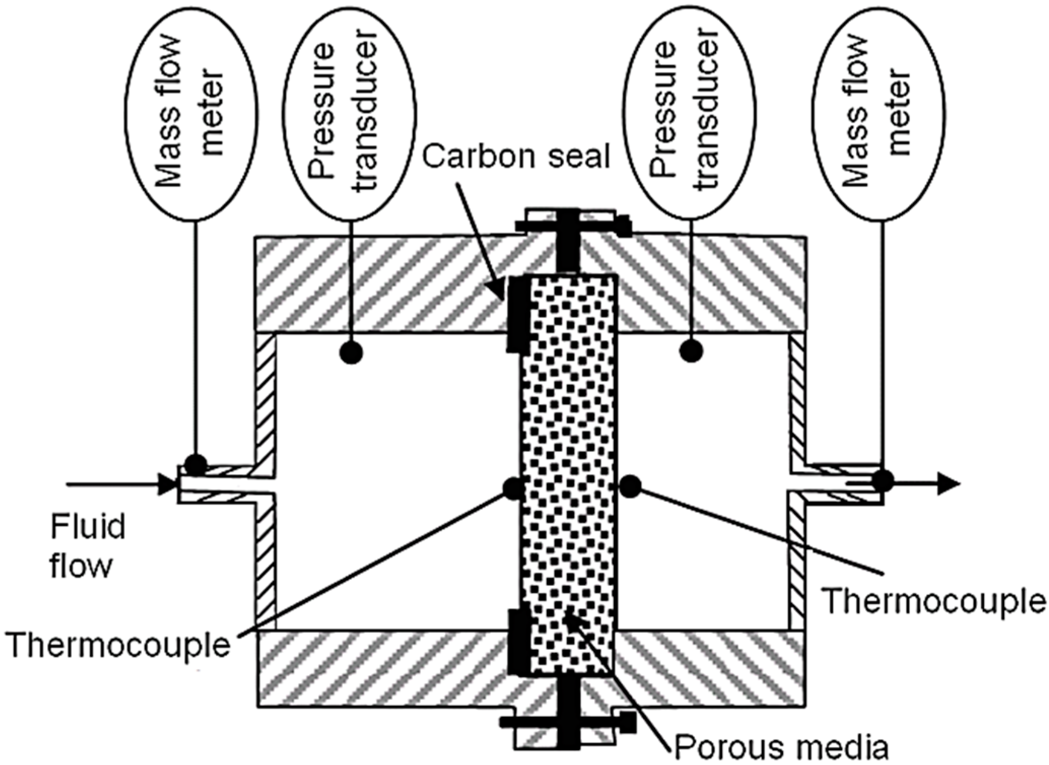
The specific test cell presented in Figure 1 is used for data generation [5]. It consists in feeding fluids into a porous material at a regulated pressure and regulated temperature. The porous material is tightened by compression between two shells and the tightness is ensured by a thermal resistant carbon seal. Each shell is instrumented with pressure sensors and thermocouples. A mass flowmeter is placed at the inlet for monitoring the fluid flow rate. Another flowmeter is placed at the outlet for mass balance control to avoid leakage in the system. Additional thermocouples can be used to control the thermal homogeneity of the test device and of the fluid. The entire system is placed into a furnace. This configuration is representative of realistic conditions found in hypersonic airbreathing vehicles. When using hydrocarbon fuel in this experiment, a high temperature generates fuel pyrolysis which results in a multispecies flow varying along the flow due to chemical reactions. One can refer to the work of Lu and Connell [54] for deeper analysis and the theoretical foundations of a multiphase and multispecies flow within porous structures. For the present work, pure nitrogen is considered for having a stable fluid under gaseous to supercritical conditions. Even if not used by the model itself, the porous medium characteristics are the following. It is 3 mm thick and made of stainless steel. It has a porosity of 30.4% and the mean grain diameter value is 14.1 µm. The complete list of sensors and of data acquisition system together with their reference can be found in [5].

The test methodology is the following. First, the fluid is fed at a given inlet pressure between 1.53 × 10⁵ Pa and 34.87 × 10⁵ Pa and at a given inlet flow rate between 0.045 g/s and 5.892 g/s. Then, the temperature of the system is set between 291 K and 1173 K. Depending on the operating conditions of the temperature and pressure during the experiments, one can observe a multispecies flow, a multiphase flow or a supercritical flow when considering hydrocarbon fuels like n-dodecane. The heating rate to reach the desired temperature is 10 K·s⁻¹. The thermal equilibrium is reached once each thermocouple value becomes stable (a time evolution lower than 0.001 K·s⁻¹). The thermal homogeneity is ensured when differences between thermocouples are lower than 2 K. For each thermal plateau, the parameters of the temperature, pressure and mass flowrate are acquired. Then, the inlet fluid pressure is increased step by step; the mass flowrate varies accordingly and the furnace regulation ensures the thermal stability. The reference viscosity is obtained in the open literature [55].

Table 1. Database characteristics for training, testing, and validating the NGPV sensor.

Database ID	Database Destination	Temperature (K)	Pressure (Pa)	Mass Flowrate (g/s)	Comments
1	Training and Testing	291–1173	1.53 × 105 Pa–7.31 × 105 Pa	0.045 g/s–0.479 g/s	514 datapoints
2	Validating	291–1173	1.78 × 105 Pa–6.87 × 105 Pa	0.090 g/s–0.440 g/s	48 datapoints
3	Validating	291–1173	7.02 × 105 Pa–34.87 × 105 Pa	0.906 g/s–5.892 g/s	47 datapoints; Supercritical state

summarizes the range of parameters which vary for each database. Depending on the test conditions, the pressure drop corresponding to these tests database ranges from 1.73 × 10⁴ Pa to 3.92 × 10⁵ Pa between the upstream and the downstream pressure transducer visible in Figure 1. Three databases are obtained by experiments: one for model training and testing with 514 datapoints and two others (48 and 47 datapoints, respectively) for validating the NGPV sensor out of its calibration range to evaluate its predictiveness and robustness.

2.2. ANN Modeling

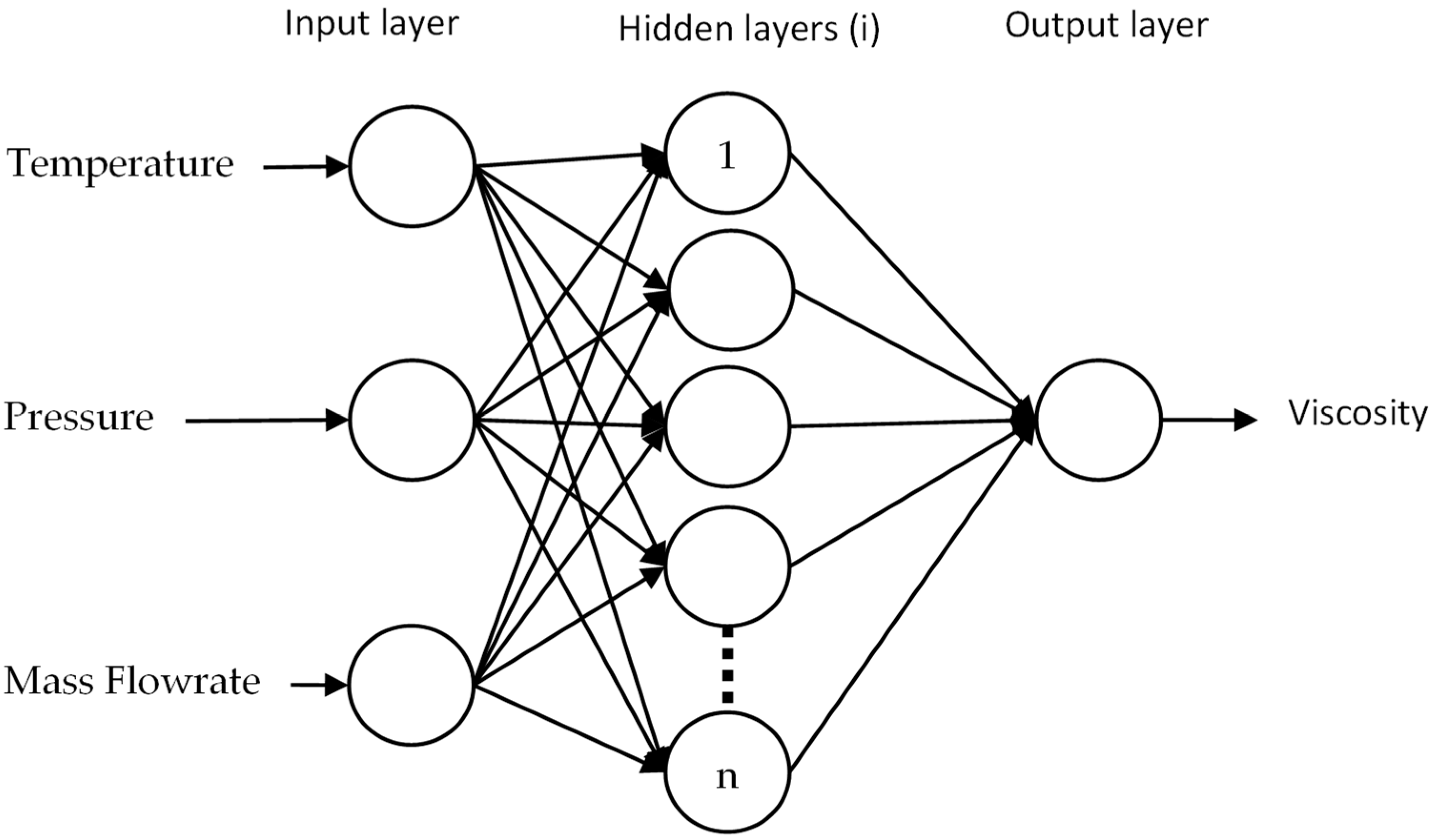
A backpropagation artificial neural network model is developed using Python scripts (version 3.12). Keras 3.0 is used for deep learning [56]. The model presents a variable number of hidden layers and a variable number of neurons per layer (Figure 2). Each layer is connected to the next one thanks to an activation function. The type of this function can be one of the following: rectified linear activation unit (ReLU), leaky_relu, softmax or linear. The input layer is fixed with a ReLU function and the output layer is fixed with a linear function. The influence of the number of iterations (epoch) and of the learning rate is evaluated on the model accuracy.

Table 2. Characteristics of the AI-based NGPV sensor.

Characteristics	Possible Values	Values Tested in the Present Work
Hidden Layers	0 and more	4; 8
Neurons	3 and more	100; 1000; 4000; 8000
Activation Functions	Linear Relu Leaky_relu Sigmoid Tanh softmax	Linear Relu Leaky_relu softmax
Learning R ates	Strictly greater than 0	10−2; 10−4; 10−8
Epochs	1 and more	Up to 1000

summarizes the training characteristics which are used in the present study. The adaptative moment estimation (Adam) optimization algorithm is used as an iterative approach in order to minimize the discrepancies between the predicted viscosity and the reference one. These discrepancies are quantified by using the mean squared error (MSE) loss function.

2.3. AI Training

After different preliminary tests, the database is randomized to consider all the available data without order so that the model is not driven by high values more than by low values. As an example, the experimental values of database #1 illustrated in

Table 3. Extraction of Database #1 presented in Table 1 for illustrative purposes.

Datapoint ID	Inlet Pressure (Pa)	Outlet Pressure (Pa)	Inlet Mass Flowrate (g/s)	Temperature (K)
1	1.78 × 105	1.61 × 105	0.090	291
[…]
8	2.64 × 105	2.03 × 105	0.212	291
[…]
17	3.28 × 105	2.47 × 105	0.313	291
[…]
76	2.27 × 105	1.66 × 105	0.094	473
[…]
255	6.87 × 105	4.22 × 105	0.440	873
[…]

are mixed and not delivered to the model in the original dataset order from 1 to 514. A total of 80% of the database #1 is dedicated to the training steps and the remaining 20% are used for testing the model. The two other databases (#2 and #3) enable us to predict the viscosity values under experimental conditions which are different from those of training and testing. This contributes to evaluating the performance and the robustness of the NGPV sensor. It shall be noticed that the input data have not been normalized in order to keep their physical significance. The MSE and MAE values are computed for each epoch both for training and for testing phases.

The fact that this work focuses on gas viscosity requires particular attention in terms of accuracy because of typical viscosity values of the order of 10⁻⁵ Pa·s. Such very low absolute values require both developing specific instrumentation and ensuring a strong reliability of each step of the physical and numerical process. As an example, the specific gas study of Hermann and Vogel [57] had to be republished after correction of some intermediate calibrations. Caponi et al. [58] developed an AI approach for hydrocarbon viscosity and obtained a mean absolute error (MAE) of 2.7.10⁻² Pa·s which is three orders of magnitude greater than the gas viscosity expected in the present study. Consequently, in the present study, it forces us to reach MSE and MAE values lower than the viscosity values themselves. Thus, an MAE convergence criterion of 6 × 10⁻⁶ Pa·s is chosen after preliminary tests.

3. Results

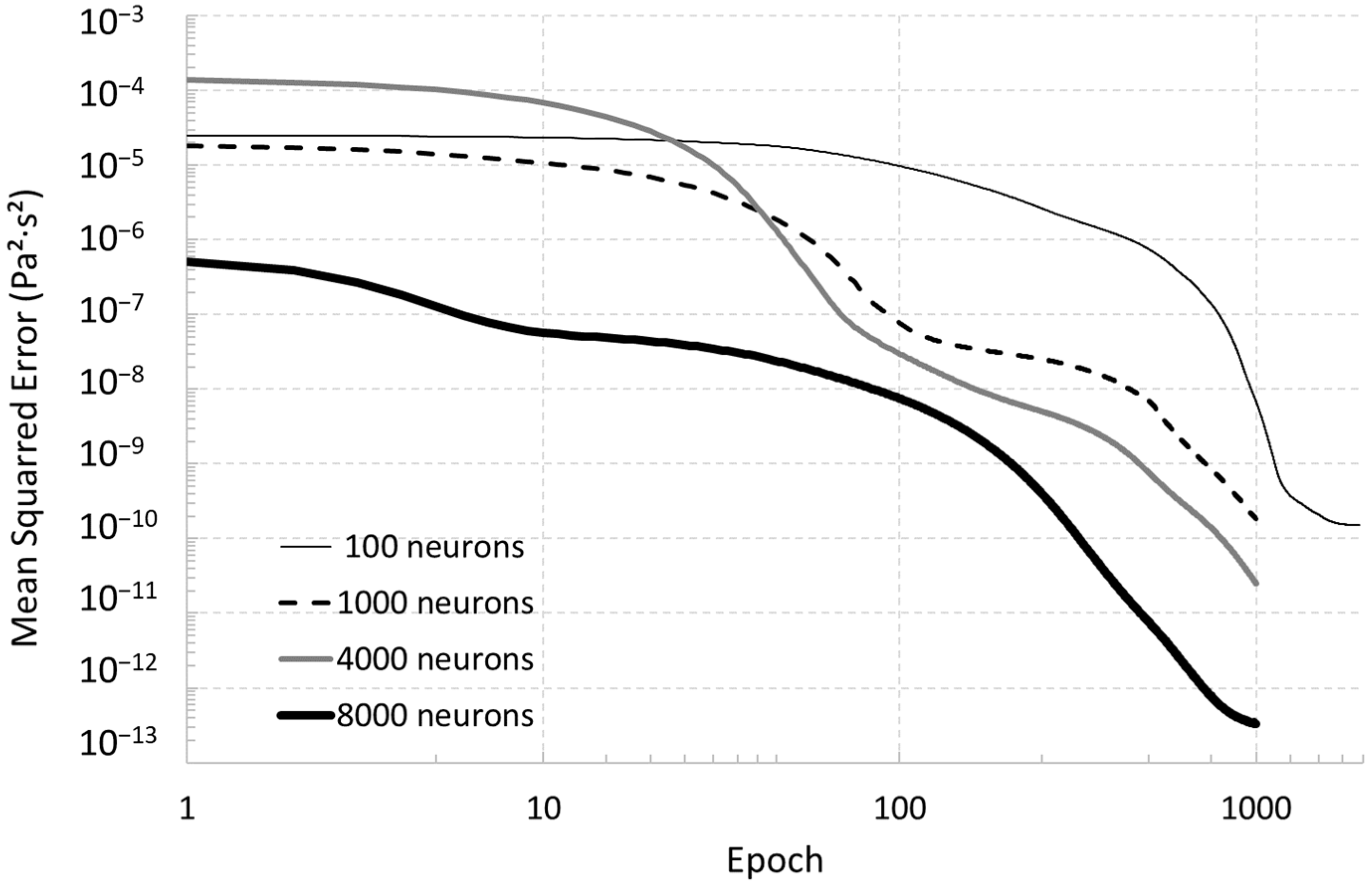
Using database #1, a parametric study was achieved on the characteristics of the NGPV sensor model in order to evaluate the most appropriate configuration. As given in Table 2, seven model configurations were tested by varying the neuron numbers (100, 1000, 4000, and 8000), the number of hidden layers (four or eight), and the learning rate (10⁻², 10⁻⁴ and 10⁻⁸). The epoch number is usually 1000 except for the 100 neurons case (1950 epochs) because of its slow convergence (Figure 3). 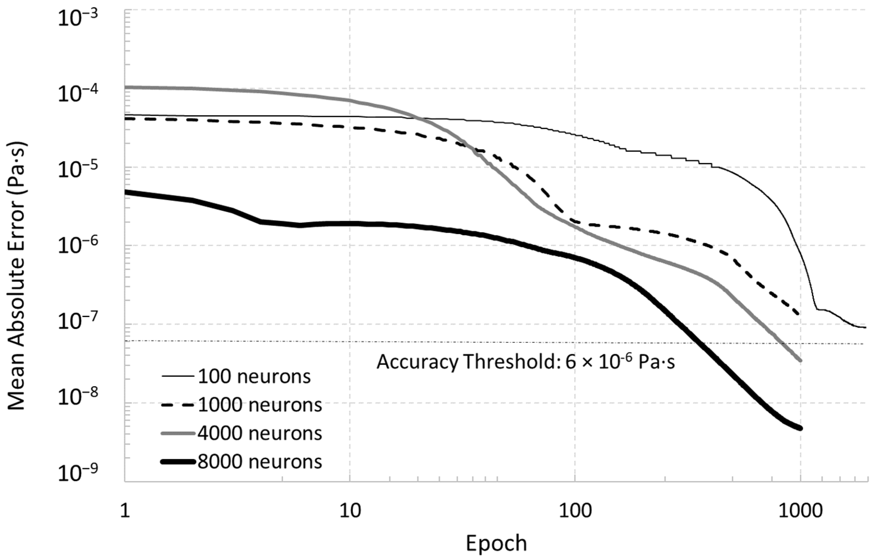As could easily be expected, the higher the epoch number is, the lower is the MSE and the higher the neurons number is, the lower is the MSE (Figure 3). Since an accuracy criterion of 6 × 10⁻⁶ Pa·s was defined in Section 2 in order to design an accurate virtualized sensor, Figure 4 shows that using 1000 neurons or fewer is not enough to respect this performance criterion. The 100 neurons configuration stagnates around 10⁻⁵ Pa·s and the 1000 neurons one may need many more epochs to go under the accuracy threshold. Indeed, Figure 4 uses a log scale and the computational effort is judged to be crippling compared to the best configurations made of 8000 neurons demonstrating a MAE as low as 4 × 10⁻⁷ Pa·s which is excellent in terms of sensitivity and accuracy for the viscosity sensors. It could be noticed that the performances of the 100 neurons case are one order of magnitude worse than the 1000 neurons case if the comparison is conducted at the same epoch number of 1000 (Figure 4).

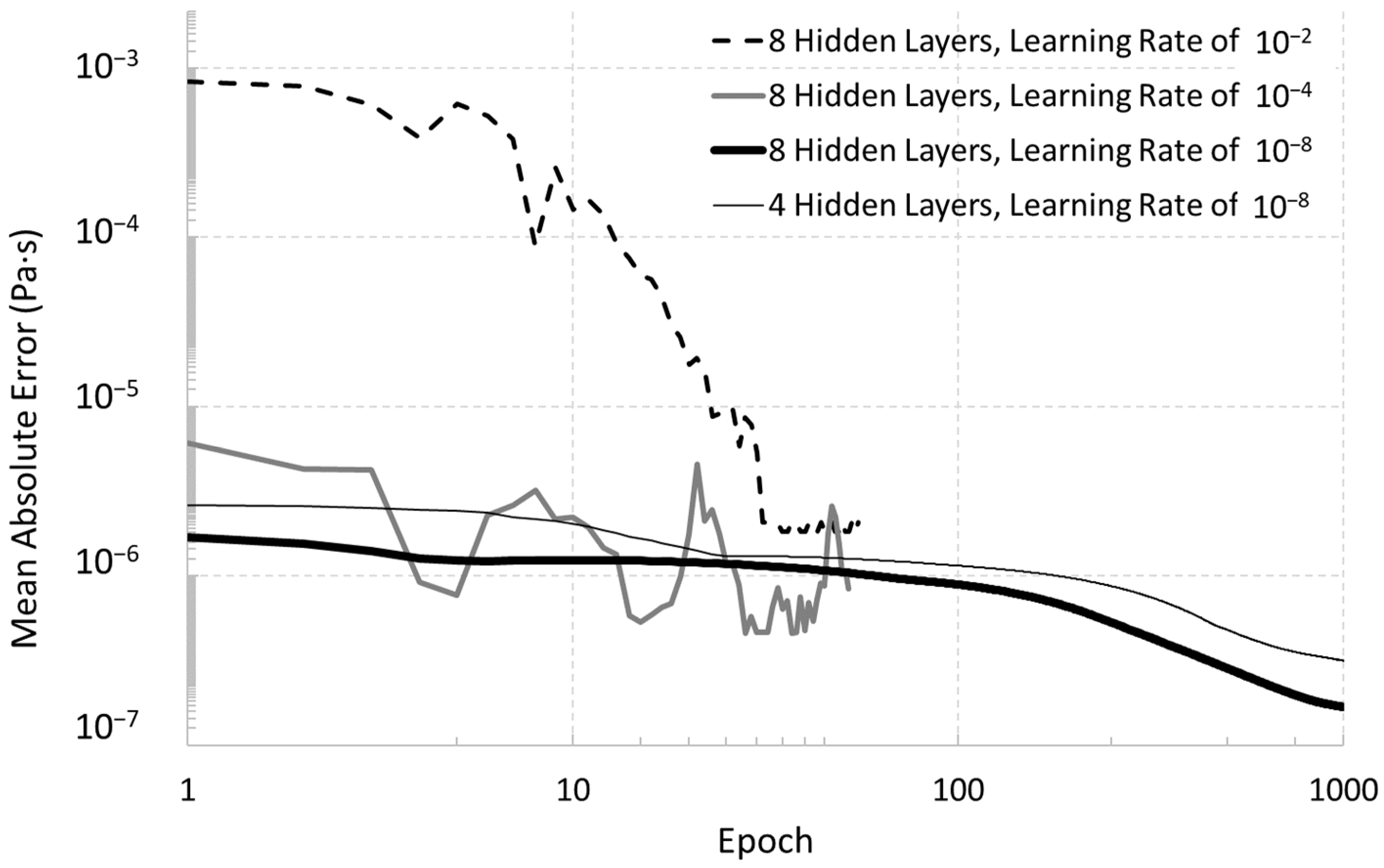
Considering this best tested configuration with 8000 neurons, the learning rate clearly impacts the performance of the model since the smallest MAE values are 6 × 10⁻⁴ Pa·s for a learning rate of 10⁻² and 10⁻⁵ Pa.s for a rate of 10⁻⁴ (Figure 5). The model convergence is erratic for these two highest learning rate values. In addition, considering four hidden layers instead of eight generates a similarly smooth convergence because of the same learning rate of 10⁻⁸. However, for four hidden layers, while its final MAE value (3 × 10⁻⁶ Pa·s) is lower than the fixed accuracy threshold, its value remains one order higher than the one for eight hidden layers.

Table 4. Number of trainable parameters depending on model characteristics.

Model ID	Number of Hidden Layers	Number of Neurons	Learning Rate	Number of Trainable Parameters	MSE (Pa2·s2)	MAE (Pa·s)	Line Slope (y/x)	R2
#1	8	100	10−8	71,301	2.0 × 10−10	9.1 × 10−6	0.9952	0.8361
#2	8	1000	10−8	7,013,001	2.7 × 10−10	1.3 × 10−5	1.0238	0.8134
#3	8	4000	10−8	128,056,001	2.1 × 10−11	3.4 × 10−6	1.0126	0.9723
#4	8	8000	10−8	448,104,001	3.9 × 10−13	4.8 × 10−7	1.0006	0.9996
#5	4	8000	10−8	192,072,001	1.7 × 10−11	3.2 × 10−6	1.0128	0.9838
#6	8	8000	10−2	448,104,001	3.9 × 10−6	8.8 × 10−4	-	-
#7	8	8000	10−4	448,104,001	3.6 × 10−9	5.9 × 10−5	-	-

summarizes the above computations made on database #1 by giving the lowest MSE and MAE values for each case. The performances are clearly linked to the number of trainable parameters because the more the parameters there are, the lower the MSE and the lower the MAE will be; except for model #1 because 1950 epochs were used for this 100 neurons case instead of 1000 for the others. In terms of model training and testing, it can be seen in Table 4 that models #3, #4, and #5 only respect the accuracy criterion on the MAE. Then, the computed viscosity values are compared for each model ID to the reference values in order to quantify their respective discrepancies with a linear regression (the two last columns of Table 4). The absence of value for models ID #6 and #7 are due to the constant output viscosity value which was computed independently from the varying input. Consequently, no linear regression could be found, and this demonstrates that these two configurations are clearly inappropriate for the development need of the NGPV sensor. For the five other model IDs, the data are presented in Figure 6 in order to observe the discrepancies. From these results, the model ID#4 with 8000 neurons, eight hidden layers and a learning rate of 10⁻⁸ is clearly the most accurate one with a slope linear coefficient of 1.0006 and a determination coefficient R² of 0.9996. Despite the other models present slope linear coefficients close to 1, their predictions are quite far from the reference values and this generates lower R² values. The model ID#5 with four hidden layers may be the only other configuration with an acceptable performance. For this reason, these two model IDs #4 and #5 are considered for further work on databases #2 and #3.

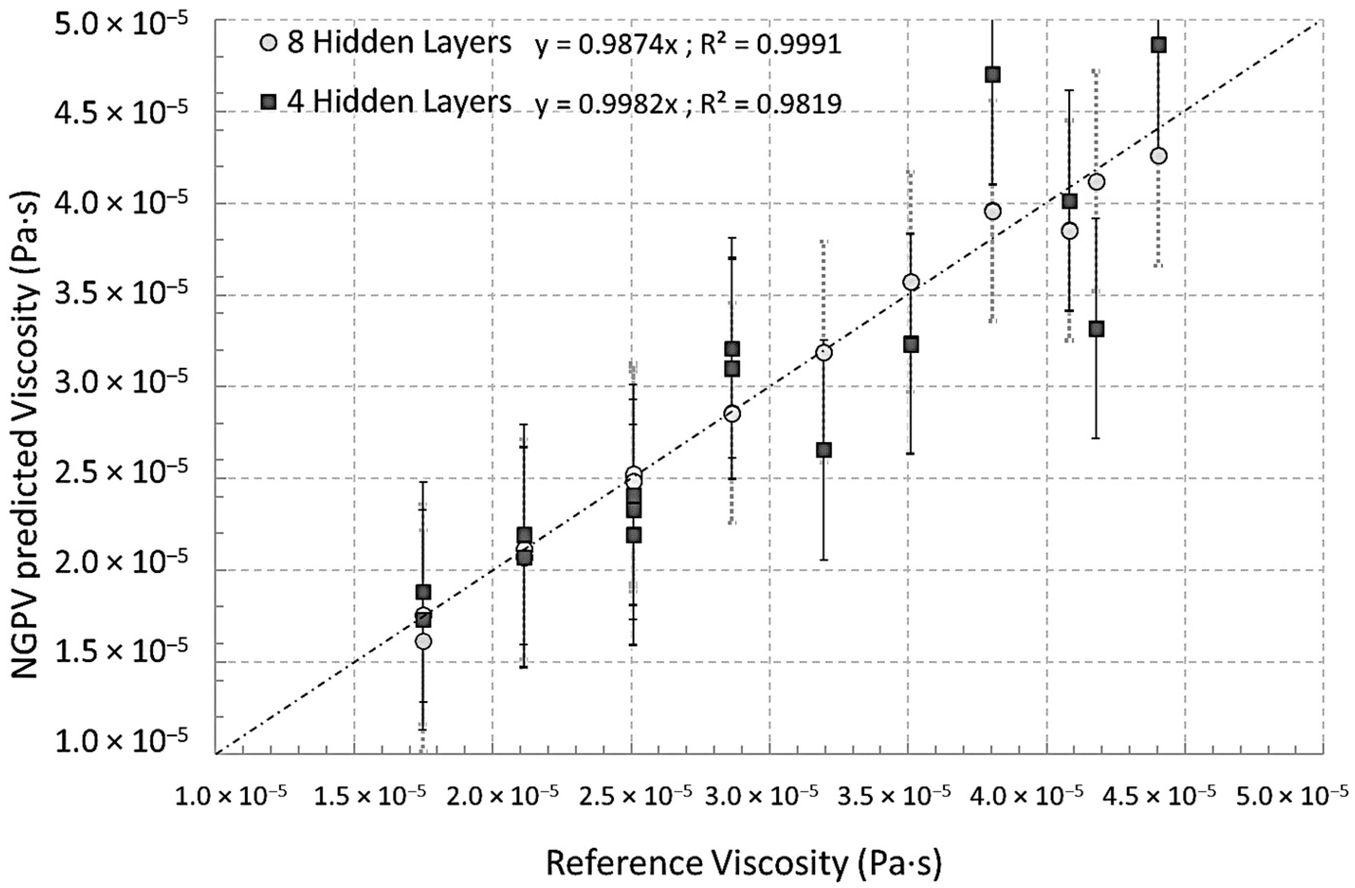
Using database #2 on unseen data, the model ID#4 (8 hidden layers) and #5 (4 hidden layers) do perform in a satisfying manner (Figure 7). The model ID#4 presents fewer variations compared to a lower number of hidden layers (model ID#5) but the differences may be considered as acceptable. By observing the operating conditions of database #2 presented above in Table 1, it can be seen that the input parameters are within the ranges of those of database #1. 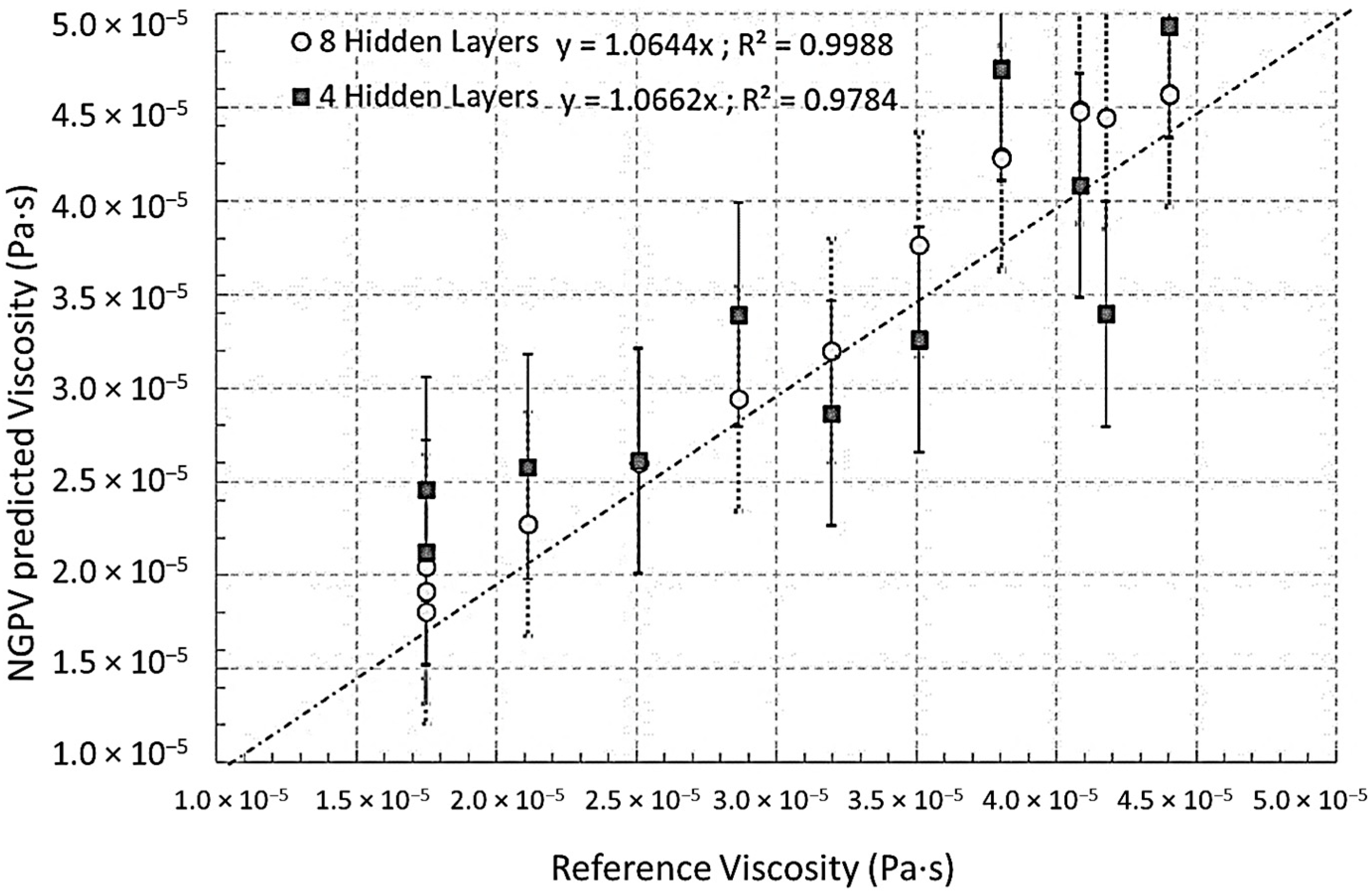Consequently, Figure 7 is related to ideal conditions for using the NGPV sensor and choosing between the two models #4 and #5 needs further investigating of the conditions out of the calibration range of the NGPV sensor. Thus, the database #3 is considered because it corresponds to conditions out of the calibration scope (Table 1). Under these unseen physical conditions, the model ID#4 definitely over-performs compared to the model ID #5 (Figure 8). The model ID#4 (R² of 0.9988) exhibits fewer variations and a better linearity compared to the model ID#5 (R² of 0.9784). This is attributed to the number of hidden layers and consequently to the number of trainable parameters which are two times greater for model ID#4 compared to model ID#5. On top of this trivial numerical observation, the following physical attention is required.

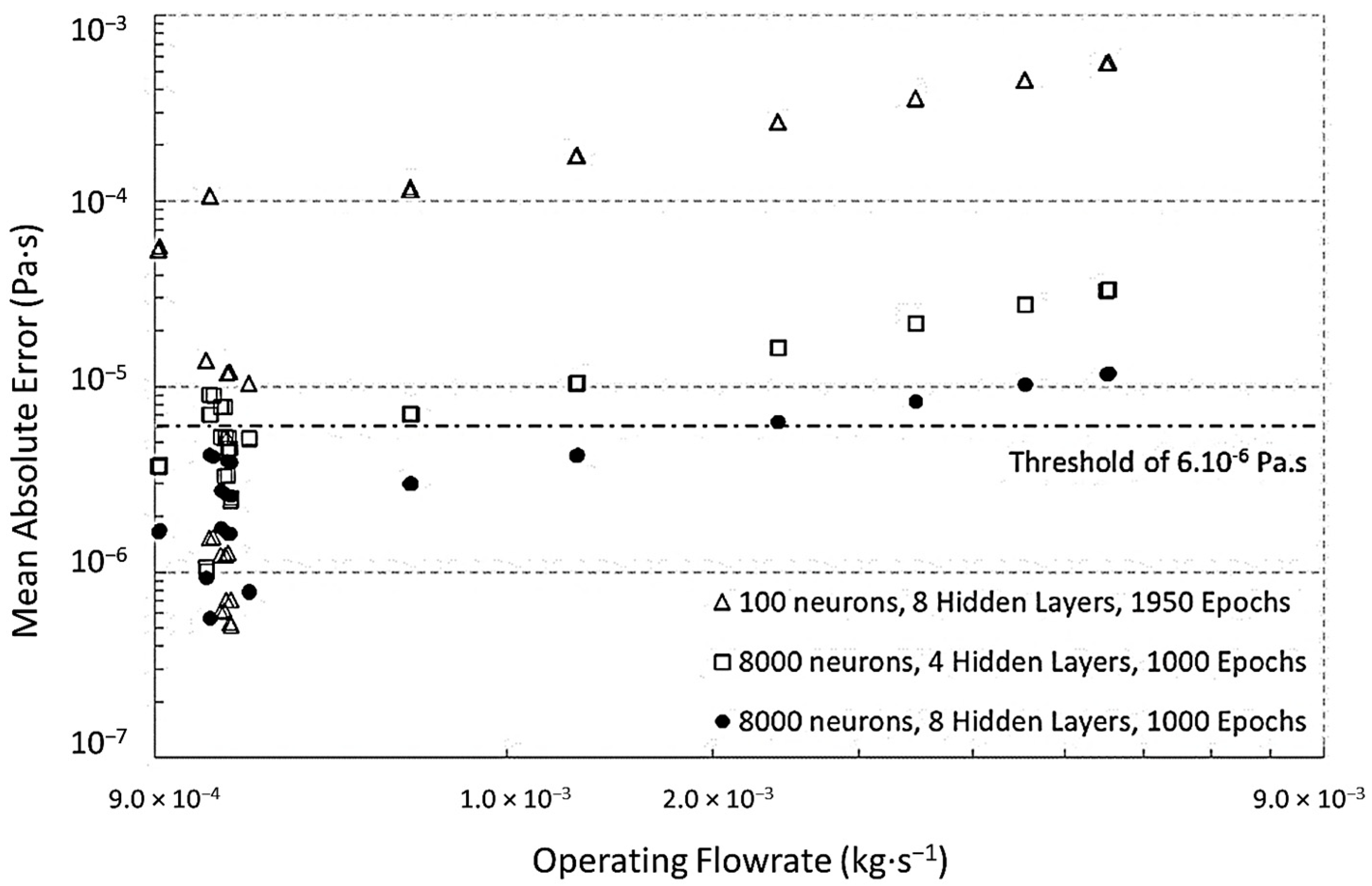
Database #3 exhibits an operating mass flowrate higher than those of the training and testing database #1 which corresponds to the calibration of the NGPV sensor. Since the physical device that the NGPV sensor is intended to virtualize corresponds to a porous material, it was mentioned earlier that the flow regime plays a role. Only low speed flows correspond to viscous Darcian flows. The higher flow speeds are related to inertial Forchheimer flows in which the viscosity relationship with the operating pressure and flowrate is modified by the squared velocity. This corresponds to the usual Brinkmann equation [5]. Consequently, it is clearly seen that the higher the flowrate is, the worse is the predicted viscosity (Figure 9). Under these conditions, the model ID#4 with 8000 neurons and eight hidden layers performs much better. It satisfies the accuracy threshold of 6 × 10⁻⁶ Pa·s up to 30 × 10⁻⁴ kg·s⁻¹ instead of only 9 × 10⁻⁴ kg·s⁻¹ for the model ID#5. This excellent result must be noticed because it shows that the model ID#4 is highly accurate for operating conditions which are 10 times higher (database #3) than those of the calibration (database #1). Additional training for higher flowrates would be required for further enlarging the ID#4 model applicability if needed. In addition, the operating pressure of database #3 reaches 34.87 × 10⁵·Pa which also slightly impacts the viscosity value even if its effect is much more limited than the thermal one (from 17.6 × 10⁻⁶ Pa·s at 293 K and 10⁵ Pa to 18.1 × 10⁻⁶ Pa·s at 293 K and 3.5 MPa).

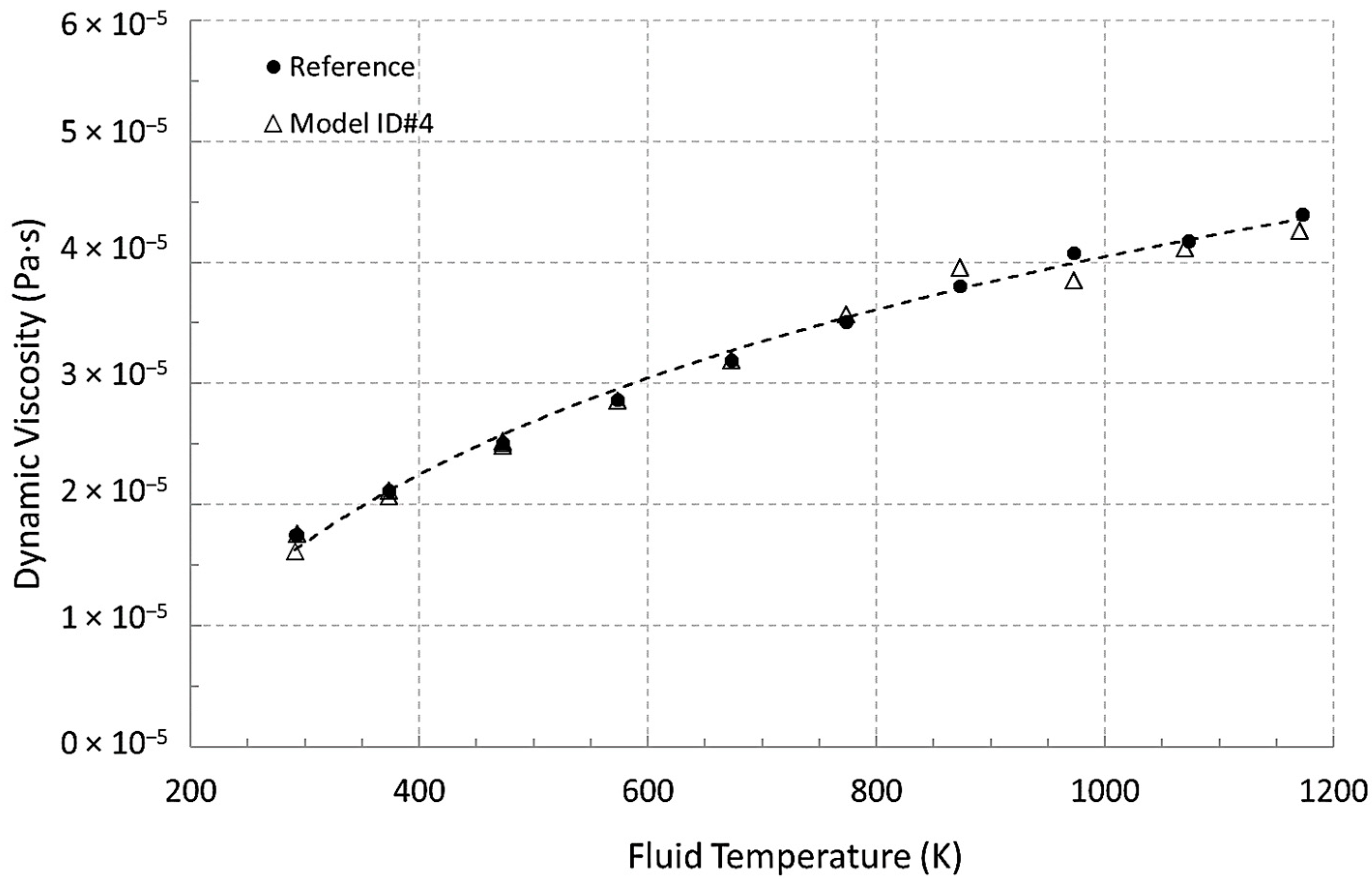
Based on the above development phases of training, of tests, and of validation, the model ID#4 is selected in order to introduce the NGPV sensor which is the first virtualized viscosity sensor to the best of the authors’ knowledge. This NGPV sensor now enables the monitoring of common parameters of industrial processes such as temperature, pressure, and flowrate in order to deliver a viscosity value of the fluid flowing in the related pipes. This avoids using dedicated online rheometers. An example of use is given in Figure 10 for a test during which the temperature increases. The fluid viscosity is monitored by the NGPV sensor and shown in Figure 10. The reference viscosity is plotted for comparison purposes. The results of this test are satisfactory and the differences between the NGPV sensor values and the reference ones are better than the expected accuracy of 6 × 10⁻⁶ Pa·s.

4. Conclusions

This paper delves deeper into the energy management metrology with a case study related to the critical process parameter, which is the dynamic viscosity of fluids. While the technologies of sensors have progressed over recent centuries, artificial intelligence (AI) today represents the next opportunity for sensors by improving the signal treatment and by extending the measurement range under operational conditions which are currently not accessible; particularly when dealing with hypersonic airbreathing technologies. An AI-based model was thus considered in this paper in order to evaluate its potential to obtain information on the fluid characteristics on the basis of basic operational parameters usually available thanks to simple and robust sensors. An experimental database containing operating process parameters like the temperature, the pressure, and the flowrate was used to train and to test seven models’ configurations. The MSE, MAE, R², and linear coefficients are the performance parameters that enabled us to select the best model configuration depending on hyperparameters like the number of hidden layers and of neurons, the learning rate and the number of epochs. It was found that the greater the number of trainable parameters (corresponding to greater hidden layers and neurons) is, the greater is the number of epochs and the lower is the learning rate and the better is the model accuracy. While the purpose of this work was to develop an AI model and not particularly to achieve the best efficiency, the work was concentrated on the accuracy of viscosity determination whatever its computational cost. The best accuracy was found accordingly for the model configuration #4 (8000 neurons, eight hidden layers, 1000 epochs, learning rate of 10⁻⁸). Even for the most extreme temperature and pressure conditions where the fluid was supercritical (1173 K and 3.5 MPa), the corresponding new generation predicted viscosity (NGPV) sensor delivered an accuracy of 4.8 × 10⁻⁷ Pa·s. This virtualized NGPV sensor was shown to be highly reliable with an accuracy of 6 × 10⁻⁶ Pa·s, even for operating flowrates 10 times higher than those of the calibration. This unprecedented result is surely to be highlighted because common viscosimeters present an accuracy around 10⁻⁴ Pa·s in their range of calibration and this drastically diverges outside the calibration range. For the NGPV sensor, over flowrate values greater than 10 times the one of calibration, it was observed that further training would be required because of the change in the flow regime from Darcian to Forchheimer. Future work may contribute to fine-tune empirical correlations often used to determine mixture properties based on data from pure components. From this perspective, a much larger database is expected to be considered in order to reinforce the robustness of the method over a large range of operating conditions and one of fluid nature.