Article

IIP-Mixer: Intra–Inter-Patch Mixing Architecture for Battery Remaining Useful Life Prediction

1
School of Computer Science and Engineering, Macau University of Science and Technology, Macau SAR, China
2
Dongguan Polytechnic, Dongguan 523808, China
*
Author to whom correspondence should be addressed.
Energies 2024, 17(14), 3553; https://doi.org/10.3390/en17143553
Submission received: 21 June 2024 / Revised: 14 July 2024 / Accepted: 17 July 2024 / Published: 19 July 2024
(This article belongs to the Section D2: Electrochem: Batteries, Fuel Cells, Capacitors)

Abstract

:
Accurately estimating the Remaining Useful Life (RUL) of lithium-ion batteries is crucial for maintaining the safe and stable operation of rechargeable battery management systems. However, this task is often challenging due to the complex temporal dynamics. Recently, attention-based networks, such as Transformers and Informer, have been the popular architecture in time series forecasting. Despite their effectiveness, these models with abundant parameters necessitate substantial training time to unravel temporal patterns. To tackle these challenges, we propose a straightforward MLP-Mixer-based architecture named “Intra–Inter Patch Mixer” (IIP-Mixer), which leverages the strengths of multilayer perceptron (MLP) models to capture both local and global temporal patterns in time series data. Specifically, it extracts information using an MLP and performs mixing operations along both intra-patch and inter-patch dimensions for battery RUL prediction. The proposed IIP-Mixer comprises parallel dual-head mixer layers: the intra-patch mixing MLP, capturing local temporal patterns in the short-term period, and the inter-patch mixing MLP, capturing global temporal patterns in the long-term period. Notably, to address the varying importance of features in RUL prediction, we introduce a weighted loss function in the MLP-Mixer-based architecture, marking the first time such an approach has been employed. Our experiments demonstrate that IIP-Mixer achieves competitive performance in battery RUL prediction, outperforming other popular time series frameworks, such as Informer and DLinear, with relative reductions in mean absolute error (MAE) of 24% and 10%, respectively.

1. Introduction

Lithium-ion batteries are widely used in electric vehicles, unmanned aerial vehicles, and grid energy storage systems. Accurate prediction of the remaining useful life (RUL) of a battery is crucial for effective battery management and health estimation [1,2]. This task is challenging due to nonlinear degradation mechanisms caused by cycling and varied operational conditions. Typically, the battery RUL is defined as the number of cycles when a battery reaches 80% of its initial capacity. Previous works on battery RUL prediction can be categorized into two main approaches: physics-based approaches and data-driven approaches [3].
Physics-based approaches such as the single-particle model [4] and the pseudo-two-dimensional model [5] based on the electrochemical principles underlying lithium-ion batteries (LIBs) can simulate the current and voltage characteristics of a battery from kinetics and transport equations. Although these models are usually precise and understandable, they come with significant computational demands and difficulties when extending their applicability to different battery cell types [6].
In contrast, data-driven approaches do not make a priori assumptions about battery degradation mechanisms but instead leverage historical cycling data of batteries. Data-driven approaches, such as Dynamic Programming Methods (DPMs) [7], are efficient and adept at handling nonlinearities, but can be complex to implement and resource intensive for large-scale problems. Gaussian processes [8,9] offer flexible, probabilistic modeling and uncertainty quantification; however, they face challenges with scalability and are computationally expensive for large datasets. Other methods incorporate intricate structures such as gating mechanisms [6,10,11] and attention mechanisms [12,13,14]. Although these approaches are effective, they often require substantial training time to thoroughly explore temporal and intercorrelation patterns, which demands extensive computing resources [15]. In addition, the permutation-invariant self-attention mechanism leads to a loss of temporal information to some extent [16].
To tackle these challenges, we propose a novel MLP-Mixer-based architecture named “Intra–Inter-Patch Mixer” (IIP-Mixer). Unlike traditional neural network-based models [17], IIP-Mixer uses multilayer perceptrons (MLPs) exclusively, which simplifies the architecture while maintaining high performance, relying solely on basic matrix multiplication routines, changes to data layout, and scalar nonlinearities [18]. The key contributions of our work are as follows:
  • Novel architecture: The IIP-Mixer architecture introduces parallel dual-head mixer layers: the intra-patch mixing MLP, which captures local temporal patterns in the short-term period, and the inter-patch mixing MLP, which captures global temporal patterns in the long-term period. This parallel dual-head approach allows the model to effectively learn from both short-term and long-term data patterns.
  • Weighted loss function: To address the varying importance of features in RUL prediction, we introduce a weighted loss function in the MLP-Mixer-based architecture. This innovation marks the first time such an approach has been employed in this context, enhancing the model’s ability to prioritize more critical features during training.
  • Performance and efficiency: Our experiments demonstrate that the IIP-Mixer achieves competitive performance in battery RUL prediction, outperforming other popular time series frameworks. Furthermore, the simplicity of the MLP-based design results in faster training times compared to attention-based models like Transformers, making it a more efficient solution for real-time applications.

2. Related Work

Remaining useful life (RUL) estimation forecasts when a battery will become ineffective, thereby minimizing risks by evaluating cell condition. This is essential for planning proper maintenance and reducing mishap risks. However, RUL estimation accuracy is often hindered by insufficient data, model complexity, and system constraints. To improve prediction accuracy, various approaches are utilized [19].

2.1. Physics-Based Approaches

Physics-based approaches examine the chemical and physical phenomena affecting battery performance, providing detailed evaluations [20]. The type of electrode material significantly influences the accuracy and effectiveness of RUL prediction methods. Graphite and lithium cobalt oxide (LCO) electrodes [21], known for their relatively predictable degradation patterns, are well suited for physics-based models. On the other hand, tin-based anodes [22] and composite materials exhibit more complex degradation behaviors and require more sophisticated modeling approaches to capture the intricacies of their performance. The intricate performance of these advanced materials over time highlights their suitability for more sophisticated predictive approaches. Physics-based approaches can be categorized into semi-empirical and empirical methods.
  • Semi-empirical methods map degradation parameters to key battery metrics like static capacity and impedance under different loads and environmental conditions through offline testing. Sankararaman et al. [23] extended the first-order second-moment method (FOSM) and first-order reliability method (FORM) for use with state space models, creating a computational framework to determine the entire probability distribution of RUL predictions. Coulombic efficiency, a critical battery parameter, is closely linked to lithium inventory loss, the main aging factor for lithium-ion batteries. Leveraging this relationship, Yang et al. [24] developed a semi-empirical model to capture capacity degradation.
  • Empirical methods continuously update their model parameters through online measurement and estimation of battery states. Given the nonlinear and non-Gaussian capacity degradation characteristics of lithium-ion batteries (LIBs), Zhang et al. [25] proposed an RUL prediction method using an exponential model and particle filter. In real environments, the discharge current of LIBs changes randomly within a charge–discharge cycle, significantly affecting battery life. Shen et al. [26] developed a two-stage Wiener process model, incorporating the unscented particle filtering algorithm, to predict the RUL considering variable discharge currents.
While physics-based methods have made significant strides in mechanism analysis, constructing a perfect battery simulation model remains challenging due to the complex interactions between components and the inherently active and nonlinear nature of battery degradation. Real-time observation of a battery’s internal conditions is difficult, complicating the development of an exact physical model [27].

2.2. Data-Driven Approaches

A data-driven approach uses operational data from advanced sensor technology to construct a degradation model for predicting the RUL. Instead of relying on accurate descriptions of the system mechanism, it utilizes data to capture the inherent degradation relationship and trend [27]. Various methods have been proposed for this purpose [28,29].
  • MLP-based architecture: A multilayer perceptron (MLP) is a type of artificial neural network with a forward structure, consisting of an input layer, an output layer, and several hidden layers. Kim et al. [30] proposed a practical State of Health (SOH) classification scheme based on an MLP, performing classification using only data from discrete life spans. Das et al. [31] introduced a multilayer perceptron-based encoder–decoder model, the Time Series Dense Encoder (TiDE), for long-term time series forecasting. This model combined the simplicity and speed of linear models with the ability to handle covariates and nonlinear dependencies.
  • RNN-based architecture: Recurrent neural networks (RNNs) are designed for processing sequential data. In [32], differential thermal voltammetry (DTV) signal analysis methods are combined with RNN-based data-driven methods to track battery degradation. De Brouwer et al. [33] introduced a continuous-time version of the Gated Recurrent Unit (GRU), built upon Ordinary Differential Equations, along with a Bayesian update network for processing sporadically observed time series.
  • Transformer-based architecture: The Transformer employs an attention network to precisely capture sequential information, thereby enhancing neural network training performance. Chen et al. [34] introduced a model based on the Transformer to tackle challenges in capturing long-term dependencies and complex degradation patterns. This model integrated a position-sensitive self-attention (PSA) unit, which improved the model’s ability to incorporate local context by focusing on positional relationships in input data at each time step. To handle noisy battery capacity data, particularly during charge/discharge cycles, Chen et al. [13] developed a Transformer-based neural network using a Denoising Auto-Encoder (DAE) to learn from corrupted input and reconstruct data, effectively processing noisy battery capacity data.
Data-driven models can adjust to diverse battery types and operational conditions without requiring extensive knowledge of underlying physical processes. However, their adaptability and robustness remain persistent challenges in practical applications. Additionally, concerns often arise regarding the sensitivity of parameter settings, which can affect model performance. The accuracy of data-driven models is heavily contingent on the quality, quantity, and representativeness of the training data; inadequate data quality may result in less reliable predictions.

3. Methods

Building on the insights from previous works, we propose a novel architecture for RUL prediction that leverages the strengths of MLPs while addressing their typical shortcomings.

3.1. Problem Formulation

For systems like lithium-ion batteries, the degradation process often spans numerous cycles, with various sensor data collected during each cycle. We address the battery RUL prediction problem as a multivariate time series prediction task. Specifically, given the historical observations X R C × L , where L is the length of the look-back window, C is the number of variables, we consider the task of predicting Y R C × N , where N is the number of subsequent time steps [35]. In this work, we focus on the case when the values of the target time series are equal to the historical observation.
Problem definition:
  • Input data: the input data consist of multiple time series variables X collected over a series of cycles, representing various sensor measurements, such as voltage, current, and capacity.
  • Output data: the output is the predicted future values Y , from which the remaining useful life of the battery can be determined.
  • Objective: the goal is to develop a model that can accurately predict the future values Y based on the historical data X .

3.2. The Framework

Inspired by the recent MLP architecture MLP-Mixer [18], which demonstrates that simple univariate linear models can outperform deep learning models like CNN and Transformer on several commonly used academic benchmarks, we extend this approach. In this paper, we explore the capabilities of MLP-based models for time series forecasting, specifically tailored to the context of long-term time series forecasting for battery RUL prediction. We present IIP-Mixer, an architecture based exclusively on MLPs. The idea behind the IIP-Mixer architecture is to separate the intra-patch mixing and inter-patch mixing to capture local temporal patterns and global temporal patterns simultaneously. Both operations are implemented with MLPs. The central architecture of the IIP-Mixer is an MLP-based design, which aggregates information from both intra-patch and inter-patch within the input series. It is worth noting that different features have different patch mixers. For univariate time series, as illustrated in Figure 1, this framework contains five major components.

3.2.1. Major Components of the Framework

Input series transformation: From the perspective of channel independence, the multivariate time series X R C × L are divided into C univariate series X ( i ) R L , i = 1 , 2 , C . These univariate series are independently fed into the IIP-Mixer model. This approach breaks down these input univariate series into smaller and structured patches. It transforms each original univariate time series from a 1D series to 2D patches while preserving their original relative positions, expressed as follows:
X ( i ) R L X ( i ) R H × W
where W represents the length of the patch, and H denotes the number of patches for each univariate series, which is a tuning hyperparameter.
Intra-patch mixing MLP: The rows in the 2D input univariate series X ( i ) represent distinct patches, while the columns denote time steps. A trainable intra-patch mixing MLP shared across all patches is employed to map each patch to a hidden space. We utilize a multilayer perceptron with a single hidden layer to capture local temporal patterns within patches. The size of output O intra ( i ) is the same as that of input X ( i ) , and the process can be summarized as the following equations [18]:
O intra ( i ) = W 2 σ W 1 X ( i )
It is essential to highlight that the parameters of the intra-patch mixing MLP shared across all patches prevent the architecture from growing too fast when increasing the length L of the look-back window and lead to significant memory savings.
Inter-patch mixing MLP: The 2D patch X ( i ) T is a transposition of X ( i ) , the rows of which represent time steps, while the columns denote distinct patches. A trainable inter-patch mixing MLP shared across all of the time steps is employed to map each time step to a hidden space. Similar to the intra-patch mixing MLP, the inter-patch mixing MLP utilizes a multilayer perceptron with a single hidden layer to capture global temporal patterns across patches. The size of output O inter ( i ) is the same as that of input X ( i ) T , and the process can be summarized as the following equations [18]:
O inter ( i ) = W 4 σ W 3 X ( i ) T
Linear projection: A linear projection is a trainable linear neural network that projects aggregated output information from the intra-patch mixing MLP and inter-patch mixing MLP to predict future time steps. Additionally, the input of the linear projection incorporates the skip connections of X ( i ) . This residual design ensures that IIP-Mixer retains the capacity of temporal linear models while still being able to exploit intra–inter-patch information. The linear projection takes an input flattened from 2D patches to 1D time series and predicts long time series sequences in a single forward operation [36], significantly enhancing inference speed. The process can be summarized by the following equations:
Y ^ ( i ) = W 5 flatten O intra ( i ) + O inter ( i )   T + X ( i )
Weighted loss function: Considering the varying importance of different variables in battery RUL prediction, to further enhance prediction performance, different from the loss function of traditional multivariate time series prediction [36], we propose to use the weighted mean square error as our loss function, which can be rewritten as:
WMSELoss = i = 1 C α i 1 N j = 1 N Y ^ j ( i ) Y j ( i ) 2
where α i represents the weight assigned to the ith variable, which is derived from the random forest feature importance measure. This measure computes the importance of a feature as the normalized total reduction in the criterion (e.g., Gini impurity for classification and variance for regression) caused by that feature. It indicates the significance of each variable in predicting the remaining useful life (RUL) of the battery.
In addition, the criterion is a function that is used to measure the quality of a split. In regression tasks, feature importance in a random forest is typically measured using the reduction in variance that each feature contributes to the splits in the trees. Each time a feature is used to split the data, the reduction in variance resulting from the split is calculated. The variance reduction can be calculated as follows:
Variance Reduction = Var ( T ) N L N Var T L + N R N Var T R
where Var ( T ) is the variance of the target feature in the parent node. Var T L and Var T R , are the variances of the target feature in the left and right child nodes, respectively, N is the number of samples in the parent node, and N L and N R are the numbers of samples in the left and right child nodes, respectively.

3.2.2. Data Processing Procedure

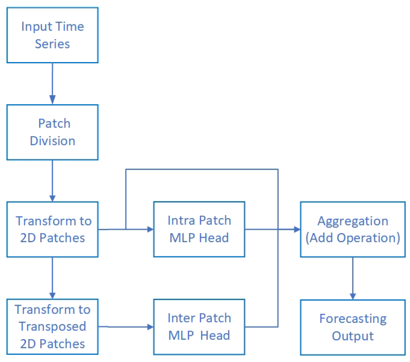
As shown in Figure 2, the time series within the look-back window, which contains historical observation data, is first divided into multiple patches. For example, a time series with 16 time steps can be divided into four patches, each containing data from 4 sequential time steps. As shown in Figure 1, the 4 different colored rectangles represent these 4 patches.
Next, we transform the 1D time series patches into 2D patches, where each row represents a distinct patch. Simultaneously, we create a transposed version of these 2D patches, with rows now representing time steps.
We then use the intra-patch MLP and inter-patch MLP to capture local temporal patterns and global temporal patterns from the 2D patches and their transposed counterparts, respectively. Following this, we aggregate the local and global temporal pattern information through an addition operation on the 2D patches.
Finally, we flatten the aggregated 2D patches back into a 1D time series and generate the forecasting output, such as the 4 sequential time steps after the look-back window, using a linear projection.

3.3. The Multivariate Time Series

In predicting the remaining useful life of rechargeable lithium-ion batteries, a lot of prior research uses only the capacity feature and barely considers more features of the battery in the charge–discharge cycles [6,13]. However, the remaining useful life (RUL) of batteries can vary significantly even among the same types of battery when subjected to different charge–discharge conditions, due to variations in temperature, voltage, and current. Consequently, predicting the RUL based solely on univariate time series data may diminish the generalization ability of the prediction model. To enhance the model’s generalization capability, it is essential to consider various load conditions by incorporating load-specific variables, such as charge voltage and charge current, into the prediction model.
To address these issues mentioned above, we propose a multivariate input representation that includes the features of charge and discharge cycles of rechargeable batteries. Scilicet, we predict the RUL of rechargeable batteries from a multivariate time series sequence. It is worth noting that feature generation and selection are crucial to the prediction performance of our proposed approach. To better capture the evolving trends in time series data, we generate a feature by calculating the mean of the accumulated capacity for each discharge cycle. Moreover, the presence of noise and redundant information in the raw measurements can impede model convergence. To address this, we introduce the random forest feature importance measure [37] to identify and incorporate the most important features, thereby improving both the convergence speed and accuracy of the model.

3.4. Dual-Head MLP

Motivated by PatchMixer [36], we employ the dual forecasting heads design in our IIP-Mixer model, including one intra-patch mixing MLP head and one inter-patch mixing MLP head.
As shown in Figure 1, the intra-patch mixing MLP head comprises two fully connected layers and a GeLU nonlinearity, facilitating communication between time steps within a patch and capturing short-term temporal dependencies. The parameters within the intra-patch mixing MLP act as the short-term memory of IIP-Mixer, emphasizing the learning of information among local time steps without considering the entire input sequence.
The structure of the inter-patch mixing MLP head is the same as that of the intra-patch mixing MLP head, allows communication between different patches, and captures temporal dependencies across the whole input sequence. It consistently processes the same time step of each patch independently, extracting long-term temporal dependencies within the entire input sequence.
It is essential to note that unlike PatchMixer, where serial dual heads are employed, our approach features parallel dual forecasting heads. As shown in Figure 2, the forecasting procedure simultaneously incorporates output information from the dual-head MLP and residual connections from past sequences to model future sequences using a linear projection. The training procedure of IIP-Mixer is summarized in Algorithm 1.
Algorithm 1: IIP-Mixer: PyTorch-like pseudocode.
# x : segments of the univariate time series
# x : the transposition of input x
# params: parameters of the network: mixer   1 : N + fc
for x in loader:                                     # load a minibatch
      x = tf ( x )                                        # transform x from 1D to 2D
      for i in range (N)                           # loop number of mixer layer
           x = mixer   i ( x )                         # the i-th mixer layer
      x = ft(x)                                         # flatten x from 2D to 1D
      pred = fc ( x )                                 # full connection layer
      loss = WMSELoss ( pred, true )  # weighted MSE loss function
      loss.backward()                            # back-propagate
      update(params)                           # SGD update
# mixer layers
def mixer (x):
      O intra = mlp intra ( x )                # intra-patch mixing MLP
      O inter = mlp inter ( x )              # inter-patch mixing MLP
      x = O intra + O inter + x            # aggregate output information
      return x

3.5. Differences between IIP-Mixer and MLP-Mixer

Different from MLP-Mixer, we made the following three modifications to enhance the model’s capability in predicting the remaining useful life of batteries:
  • First, in IIP-Mixer, unlike MLP-Mixer’s patches and features, the two dimensions represent patches and time steps, allowing us to capture both local and global temporal patterns simultaneously. Particularly, the global temporal patterns captured from time steps are crucial for battery RUL prediction, as demonstrated in Table 5.
  • Second, unlike MLP-Mixer’s serial structure of dual-head MLP, in IIP-Mixer, we introduce a parallel structure for inter-patch mixing and intra-patch mixing to capture temporal patterns simultaneously. As shown in Table 6, the parallel heads’ structure clearly outperforms the serial structure in battery RUL prediction.
  • Consequently, unlike MLP-Mixer’s traditional loss function, we propose a weighted mean square error loss function that accounts for the varying importance of features in battery RUL prediction. This approach results in a 5% relative improvement in MAE.

4. Experiments

To evaluate the effectiveness of our proposed method, we conducted experiments using a well-established dataset and compared our model’s performance against several baselines.

4.1. Datasets

We conducted our experiments using PyTorch on the public NASA PCoE battery dataset, available from the NASA Ames Research Center website. This dataset includes four Li-ion batteries (B0005, B0006, B0007, and B0018) that were subjected to three different operational profiles (charge, discharge, and impedance) at room temperature. Charging was performed in a constant current (CC) mode at 1.5 A until the battery voltage reached 4.2 V, followed by a constant voltage (CV) mode until the charge current dropped to 20 mA. Discharging was conducted at a constant current (CC) level of 2 A until the battery voltage fell to 2.7 V, 2.5 V, 2.2 V, and 2.5 V for batteries B0005, B0006, B0007, and B0018, respectively. Repeated charge and discharge cycles accelerated the aging of the batteries. The experiments were halted when the batteries met the end-of-life (EOL) criteria, defined as a 30% reduction in rated capacity (from 2 Ahr to 1.4 Ahr). We uniformly collected data only before their discharge capacity decayed to 0.55 Ah, at which point they had cycled 167, 167, 167, and 131 times, respectively.
This dataset can be used to predict the remaining useful life (RUL) of batteries. To ensure the robustness of the model, the dataset was divided into training, validation, and test sets. The training set, comprising data from B0005 and B0006, was used to fit the model. The validation set, consisting of data from B0007, was used to tune the hyperparameters. Finally, the test set, containing data from B0018, was used to evaluate the model’s performance.

4.2. Baselines

We benchmarked our IIP-Mixer models against commonly used basic networks, including MLP, Transformer models, and their newly proposed variants such as DLinear [16] and Informer [38].
  • MLP: A multilayer perceptron is like a mathematical function that maps input and output values. Multiple layers are used to learn the battery’s dynamic and nonlinear degradation trend.
  • Transformer: Transformer is a model that uses an attention mechanism for model training; it mainly consists of two components: an encoder and a decoder, with which we can predict the capacity degradation trend of the battery.
  • Informer: A variant of the Transformer architecture that efficiently handles extremely long input sequences by highlighting the dominating attention by halving the cascading layer input. It predicts the long time series sequences in one forward operation rather than in a step-by-step way, which drastically improves the inference speed.
  • DLinear: In consideration of permutation-invariant and “anti-ordering” to some extent of the Transformer-based architecture [16], DLinear decomposes the time series into a trend and a remainder series and employs two one-layer linear networks to extract the temporal relations among an ordering set of continuous points.

4.3. Implementation

4.3.1. Parameter Selection and Optimization

  • MLP: The MLP model was configured with one hidden layer. The optimal values for the learning rate and hidden dimension were determined through a grid search, resulting in 0.0005 and 32, respectively.
  • Transformer and Informer models utilized two encoder layers and one decoder layer, each with 8 attention heads. The optimal values for the learning rate, hidden dimension, and dropout rate, identified through a grid search, were 0.0001, 512, and 0.05, respectively.
  • For the DLinear model, we adopted the architecture parameters proposed in the original paper. The best performance was achieved with a decomposition kernel size of 25 and a learning rate of 0.0015, as determined through a grid search.
  • IIP-Mixer: Our model includes six key parameters: patch size, learning rate, dropout rate, patch length, number of mixer blocks, and number of principal features of the time series. The optimal values, determined through a grid search, were 4, 0.001, 0.05, 4, 1, and 6, respectively. Detailed information about the training process is provided in Table 1.
In short, we adopted the default architecture of Transformer, Informer, and DLinear proposed in [16]. For simplicity, a single hidden layer was used in both the MLP and IIP-Mixer models. To ensure a fair comparison, we standardized the input time step length to 16 and the output time step length to 4 across all models, following the methodology outlined in [13]. Additionally, to ensure the robustness of the results, each model’s hyperparameters were fine-tuned through a comprehensive grid search, and the models were evaluated using the validation set to mitigate overfitting and provide a reliable performance estimate.

4.3.2. Evaluation Metrics

In our experiments, four evaluation metrics were used to compare the performance of these models mentioned above. In addition to three common metrics, the Mean Absolute Error (MAE), Root-Mean-Square Error (RMSE), and Mean Absolute Percentage Error(MAPE) [39], we chose the Absolute Relative Error (ARE) [13] to evaluate the prediction performance of the battery RUL, which is defined as follow:
A R E = R U L p r e R U L t u r e R U L t u r e × 100 %
where R U L t u r e denotes the true RUL of the battery, and R U L p r e denotes the prediction of the RUL from models. Additionally, we conducted each experiment three times using three consecutive seeds and reported the mean of the evaluation metrics.

5. Results

5.1. Performance of IIP-Mixer

Despite its simplicity, IIP-Mixer achieved competitive results. To verify the performance of our methods, we conducted our experiments on four baseline methods. The MAE, RMSE, MAPE, and ARE scores obtained for all methods are shown in Table 2, the best results are shown in bold. All experiments in this subsection were conducted on the same machine, utilizing a single GPU (NVIDIA Tesla T4) for consistent and reliable findings. From the result, we conclude the following:
  • The Transformer and its variant, the Informer model, excel in modeling both long-term and short-term dependencies, showcasing superior performance on long-time series data. However, it is worth noting that they can easily lead to overfitting for small datasets, such as the NASA PCoE battery dataset.
  • The MPL model is adept at capturing global temporal patterns but may struggle to capture local temporal patterns from time series data. Consequently, its performance remained average across all evaluation metrics compared to other methods.
  • The DLinear model decomposes the time series into a trend and a remainder series. It utilizes two one-layer linear networks to extract temporal relations among an ordered set of continuous points, making it adept at capturing both the trend and season of a time series.
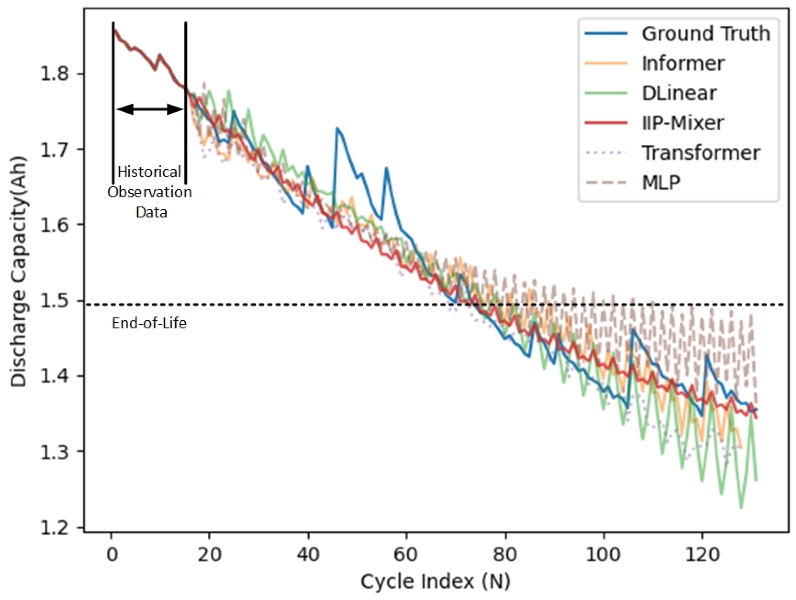
  • Among all the baseline methods, our proposed model IIP-Mixer achieved the best experimental results. As shown in Figure 3, IIP-Mixer could capture the local and global temporal patterns in time series data; this is a great help for battery RUL prediction, especially in the overall degeneration trend of discharge capacity.
Table 3 shows our model outperformed all baseline methods significantly; we achieved the best performance across all the metrics on the NASA PCoE battery dataset. IIP-Mixer demonstrated an overall relative reduction of 40% in the RMSE, 48% in the MAE, and 94% in the ARE in comparison to the state-of-the-art DeTransformer. From the result, we conclude the following:
  • LSTM and its variants, the GRU [40] and Dual-LSTM [41] models, are types of neural networks designed for processing sequential data. These models can handle examples of varying lengths by sharing parameters across different parts of the network. However, recurrent neural networks, including LSTM networks, can experience performance degradation due to long-term dependencies, which impacts their effectiveness in battery RUL prediction.
  • DeTransformer [13], a variant of Transformer, leverages the strength of the self-attention mechanism, excelling at extracting semantic correlations between paired elements in a long sequence, regardless of their order, thanks to its permutation-invariant nature. However, in time series analysis, the primary focus is on modeling the temporal dynamics among a continuous set of points, where the order of the data points is crucial [16]. This affects the effectiveness of Transformers in predicting battery RUL.
  • IIP-Mixer, a straightforward MLP-Mixer-based architecture, is well suited for learning temporal patterns due to its time-step-dependent characteristics, as demonstrated by recent work [35]. Our results also highlight the importance of efficiently utilizing MLPs to capture both local and global temporal information, thereby improving the performance of time series forecasting. In summary, this approach achieved superior performance compared to RNN-based and Transformer-based architectures.

5.2. Computation Efficiency

We investigated the computational efficiency of all neural networks mentioned above based on the length L of the input time series. Comparisons of theoretical time complexity and memory usage [38] are summarized in Table 4. It is important to note that, in our model, the patch size W can equal the patch number H, so we have W × H = W 2 = H 2 = L . It is evident that our model, like DLinear, had the lowest cost across all computational metrics.

5.3. Ablation Study

5.3.1. Effect of Dual-Head MLP

To evaluate the effectiveness of the dual-head MLP, we individually removed the intra-patch mixing MLP head or inter-patch mixing MLP head. Table 5 demonstrates that the dual-head MLP mechanism outperformed all other configurations. This result highlights the effectiveness of the dual-head mechanism in comparison to a single output head.
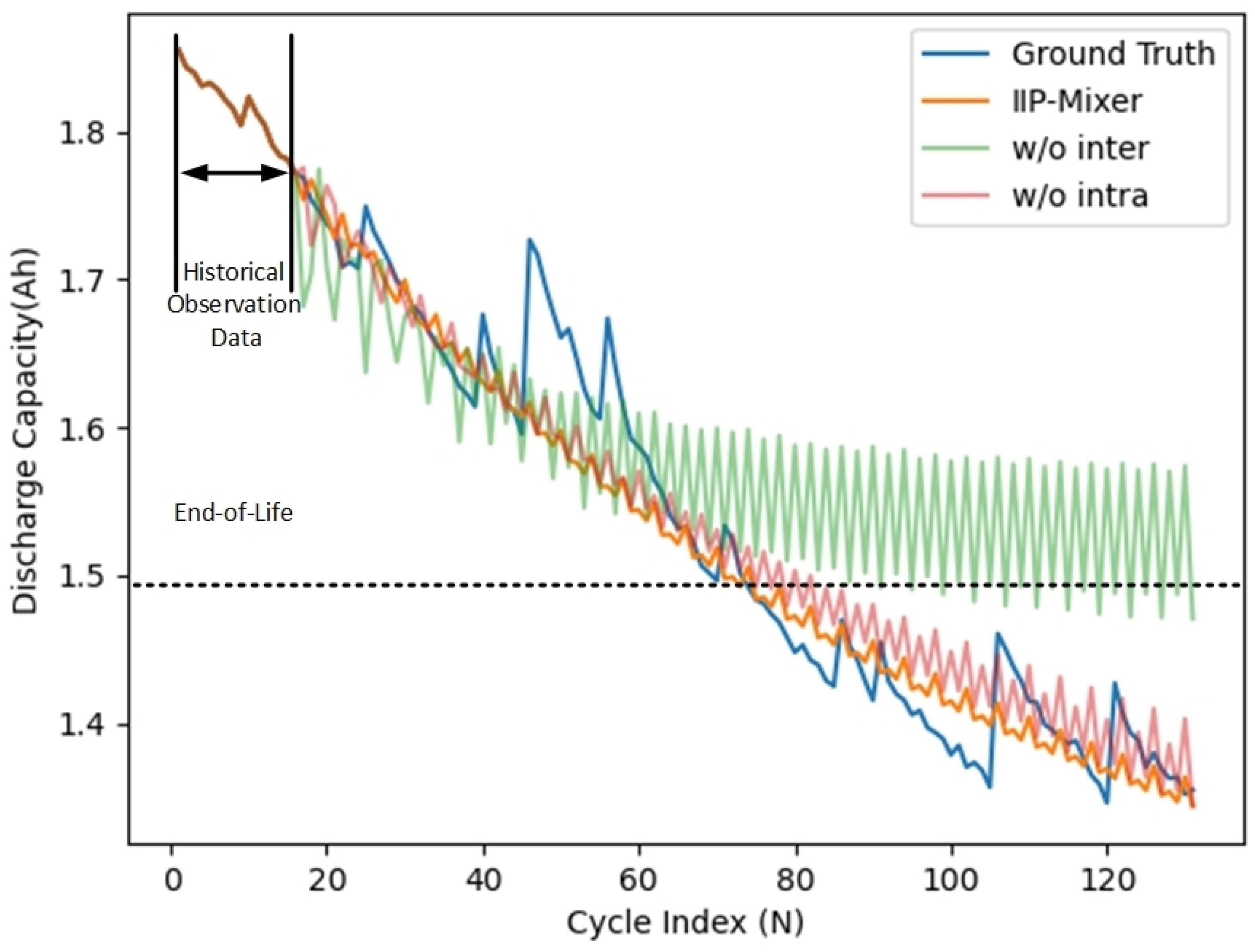
It is worth noting that as shown in Figure 4, the performance of the architecture without an intra-patch mixing MLP head was better than that without an inter-patch mixing MLP head. Specifically, the intra-patch mixing MLP conducts per-location (intra-patch) operations, capturing local temporal patterns from a single patch and identifying the short-term seasonal component of the time series. Conversely, the inter-patch mixing MLP performs cross-location (inter-patch) operations, capturing global temporal patterns from the same time step across several patches, thereby identifying the long-term trend component of the time series. In the context of battery RUL prediction, the long-term trend component contributes significantly more to predicting battery life than the seasonal component. As shown in Table 5, the inter-patch mixing MLP achieved a lower ARE of 5.02% compared to the intra-patch mixing MLP, which had an ARE of 34.70%. Naturally, the best performance was achieved with the dual-head MLP with an ARE of 1.37%.

5.3.2. Serial vs. Parallel Heads

Unlike the serial structure of the dual-head MLP in MLP-Mixer and PatchMixer, we introduced a parallel structure for dual heads. To evaluate the effectiveness of the parallel heads structure, we compared the performance of serial heads (intra-first), serial heads (inter-first), and parallel heads. As shown in Table 6, it is evident that the parallel heads’ structure outperformed the serial structure in battery RUL prediction.

5.3.3. Effect of Weighted Loss Function

In the majority of recent research on MLP-based models, the loss functions did not take into account the varying importance of different variables. As shown in Table 7, it is evident that the weighted loss function outperformed the loss function without weighting, resulting in relative improvements of 5%, 2%, and 3% in Mean Absolute Error (MAE), Root-Mean-Square Error (RMSE), and Mean Absolute Percentage Error (MAPE), respectively.

5.3.4. Effect of Multivariate Time Series

We investigated the impact of multivariate time series in Table 8. The learning performance with principal-feature multivariate time series surpassed that of univariate time series. Specifically, predicting the remaining useful life of batteries using a multivariate time series of principal features significantly enhanced the generalization ability of the prediction model.
It is important to highlight that training with multivariate time series containing all features may lead to a reduction in model performance. Therefore, the feature selection pipeline plays a critical role in determining prediction performance.

6. Conclusions

In this paper, we presented IIP-Mixer, an innovative MLP-Mixer-based architecture designed to predict the remaining useful life in batteries. IIP-Mixer incorporates a parallel dual-head MLP: the intra-patch mixing MLP and inter-patch mixing MLP. The intra-patch mixing MLP independently applies an MLP to each patch, capturing local temporal patterns in the short-term period. On the other hand, the inter-patch mixing MLP applies an MLP across all patches from the input sequence, capturing global temporal patterns in the long-term period. Moreover, recognizing the varying importance of features in RUL prediction, we proposed a weighted mean square error loss function to enhance prediction accuracy, which resulted in a 5% relative improvement in MAE. Our experiments demonstrated that IIP-Mixer achieved competitive performance in battery RUL prediction, outperforming other popular time series frameworks, such as Informer and DLinear, with relative improvements in MAE of 24% and 10%, respectively.

Author Contributions

Validation, J.G.; Investigation, Y.C.; Resources, Y.C.; Writing—original draft, G.Y.; Visualization, J.G.; Project administration, L.F.; Funding acquisition, L.F. All authors have read and agreed to the published version of the manuscript.

Funding

This research was funded by the Science and Technology Development Fund, Macau SAR, grant number 0093/2022/A2, 0076/2022/A2, and 0008/2022/AGJ, and the National Natural Science Foundation of China, grant number 61872452. It was also supported by the Guangdong Provincial Department of Education’s Key Special Projects, with project numbers 2022ZDZX1073 and 2023ZDZX1086, as well as by the Special Fund for Dongguan’s Rural Revitalization Strategy, under number 20211800400102. Furthermore, support was provided by the Dongguan Sci-tech Commissioner Program, with grant numbers 20221800500842, 20221800500632, 20221800500822, 20221800500792, and 20231800500442. Additionally, it received support from the Dongguan Science and Technology of Social Development Program, under number 20231800936942. Finally, funding was provided by the Dongguan Songshan Lake Enterprise Special Envoy Project.

Data Availability Statement

The data presented in this study are openly available in “Battery Data Set” at https://www.nasa.gov/intelligent-systems-division/discovery-and-systems-health/pcoe/pcoe-data-set-repository/.

Conflicts of Interest

The authors declare no conflicts of interest.

References

  1. Alsuwian, T.; Ansari, S.; Zainuri, M.A.A.M.; Ayob, A.; Hussain, A.; Lipu, M.H.; Alhawari, A.R.; Almawgani, A.; Almasabi, S.; Hindi, A.T. A Review of Expert Hybrid and Co-Estimation Techniques for SOH and RUL Estimation in Battery Management System with Electric Vehicle Application. Expert Syst. Appl. 2024, 246, 123123. [Google Scholar] [CrossRef]
  2. Wei, M.; Gu, H.; Ye, M.; Wang, Q.; Xu, X.; Wu, C. Remaining useful life prediction of lithium-ion batteries based on Monte Carlo Dropout and gated recurrent unit. Energy Rep. 2021, 7, 2862–2871. [Google Scholar] [CrossRef]
  3. Xu, Q.; Wu, M.; Khoo, E.; Chen, Z.; Li, X. A hybrid ensemble deep learning approach for early prediction of battery remaining useful life. IEEE/CAA J. Autom. Sin. 2023, 10, 177–187. [Google Scholar] [CrossRef]
  4. Santhanagopalan, S.; Guo, Q.; Ramadass, P.; White, R.E. Review of models for predicting the cycling performance of lithium-ion batteries. J. Power Sources 2006, 156, 620–628. [Google Scholar] [CrossRef]
  5. Kemper, P.; Li, S.E.; Kum, D. Simplification of pseudo two-dimensional battery model using dynamic profile of lithium concentration. J. Power Sources 2015, 286, 510–525. [Google Scholar] [CrossRef]
  6. Wang, J.; Zhang, S.; Li, C.; Wu, L.; Wang, Y. A data-driven method with mode decomposition mechanism for remaining useful life prediction of lithium-ion batteries. IEEE Trans. Power Electron. 2022, 37, 13684–13695. [Google Scholar] [CrossRef]
  7. Guo, H.; Liu, X.; Song, L. Dynamic programming approach for segmentation of multivariate time series. Stoch. Environ. Res. Risk Assess. 2015, 29, 265–273. [Google Scholar] [CrossRef]
  8. Roberts, S.; Osborne, M.; Ebden, M.; Reece, S.; Gibson, N.; Aigrain, S. Gaussian processes for time-series modelling. Philos. Trans. R. Soc. A: Math. Phys. Eng. Sci. 2013, 371, 20110550. [Google Scholar] [CrossRef] [PubMed]
  9. Hernández-Lobato, J.M.; Lloyd, J.R.; Hernández-Lobato, D. Gaussian process conditional copulas with applications to financial time series. Adv. Neural Inf. Process. Syst. 2013, 2, 1736–1744. [Google Scholar]
  10. Wang, S.; Fan, Y.; Jin, S.; Takyi-Aninakwa, P.; Fernandez, C. Improved anti-noise adaptive long short-term memory neural network modeling for the robust remaining useful life prediction of lithium-ion batteries. Reliab. Eng. Syst. Saf. 2023, 230, 108920. [Google Scholar] [CrossRef]
  11. Rincón-Maya, C.; Guevara-Carazas, F.; Hernández-Barajas, F.; Patino-Rodriguez, C.; Usuga-Manco, O. Remaining Useful Life Prediction of Lithium-Ion Battery Using ICC-CNN-LSTM Methodology. Energies 2023, 16, 7081. [Google Scholar] [CrossRef]
  12. Zhang, J.; Huang, C.; Chow, M.Y.; Li, X.; Tian, J.; Luo, H.; Yin, S. A data-model interactive remaining useful life prediction approach of lithium-ion batteries based on PF-BiGRU-TSAM. IEEE Trans. Ind. Inform. 2023, 20, 1144–1154. [Google Scholar] [CrossRef]
  13. Chen, D.; Hong, W.; Zhou, X. Transformer network for remaining useful life prediction of lithium-ion batteries. IEEE Access 2022, 10, 19621–19628. [Google Scholar] [CrossRef]
  14. Han, Y.; Li, C.; Zheng, L.; Lei, G.; Li, L. Remaining useful life prediction of lithium-ion batteries by using a denoising transformer-based neural network. Energies 2023, 16, 6328. [Google Scholar] [CrossRef]
  15. Ye, J.; Gu, J.; Dash, A.; Deek, F.P.; Wang, G.G. Prediction with time-series mixer for the S&P500 index. In Proceedings of the 2023 IEEE 39th International Conference on Data Engineering Workshops (ICDEW), Anaheim, CA, USA, 3–7 April 2023; pp. 20–27. [Google Scholar]
  16. Zeng, A.; Chen, M.; Zhang, L.; Xu, Q. Are transformers effective for time series forecasting? In Proceedings of the AAAI Conference on Artificial Intelligence, Washington, DC, USA, 7–14 February 2023; Volume 37, pp. 11121–11128. [Google Scholar] [CrossRef]
  17. Wei, Y.; Wu, D. State of health and remaining useful life prediction of lithium-ion batteries with conditional graph convolutional network. Expert Syst. Appl. 2024, 238, 122041. [Google Scholar] [CrossRef]
  18. Tolstikhin, I.O.; Houlsby, N.; Kolesnikov, A.; Beyer, L.; Zhai, X.; Unterthiner, T.; Yung, J.; Steiner, A.; Keysers, D.; Uszkoreit, J.; et al. Mlp-mixer: An all-mlp architecture for vision. Adv. Neural Inf. Process. Syst. 2021, 34, 24261–24272. [Google Scholar]
  19. Hasib, S.A.; Islam, S.; Chakrabortty, R.K.; Ryan, M.J.; Saha, D.K.; Ahamed, M.H.; Moyeen, S.I.; Das, S.K.; Ali, M.F.; Islam, M.R.; et al. A comprehensive review of available battery datasets, RUL prediction approaches, and advanced battery management. IEEE Access 2021, 9, 86166–86193. [Google Scholar] [CrossRef]
  20. Barré, A.; Deguilhem, B.; Grolleau, S.; Gérard, M.; Suard, F.; Riu, D. A review on lithium-ion battery ageing mechanisms and estimations for automotive applications. J. Power Sources 2013, 241, 680–689. [Google Scholar] [CrossRef]
  21. Shchegolkov, A.; Komarov, F.; Lipkin, M.; Milchanin, O.; Parfimovich, I.; Shchegolkov, A.; Semenkova, A.; Velichko, A.; Chebotov, K.; Nokhaeva, V. Synthesis and study of cathode materials based on carbon nanotubes for lithium-ion batteries. Inorg. Mater. Appl. Res. 2021, 12, 1281–1287. [Google Scholar] [CrossRef]
  22. Kamali, A.R.; Fray, D.J. Tin-based materials as advanced anode materials for lithium ion batteries: A review. Rev. Adv. Mater. Sci. 2011, 27, 14–24. [Google Scholar]
  23. Sankararaman, S.; Daigle, M.J.; Goebel, K. Uncertainty quantification in remaining useful life prediction using first-order reliability methods. IEEE Trans. Reliab. 2014, 63, 603–619. [Google Scholar] [CrossRef]
  24. Yang, F.; Song, X.; Dong, G.; Tsui, K.L. A coulombic efficiency-based model for prognostics and health estimation of lithium-ion batteries. Energy 2019, 171, 1173–1182. [Google Scholar] [CrossRef]
  25. Zhang, L.; Mu, Z.; Sun, C. Remaining useful life prediction for lithium-ion batteries based on exponential model and particle filter. IEEE Access 2018, 6, 17729–17740. [Google Scholar] [CrossRef]
  26. Shen, D.; Wu, L.; Kang, G.; Guan, Y.; Peng, Z. A novel online method for predicting the remaining useful life of lithium-ion batteries considering random variable discharge current. Energy 2021, 218, 119490. [Google Scholar] [CrossRef]
  27. Su, C.; Chen, H. A review on prognostics approaches for remaining useful life of lithium-ion battery. In Proceedings of the IOP Conference Series: Earth and Environmental Science; 2017; Volume 93, p. 012040. [Google Scholar]
  28. Safavi, V.; Mohammadi Vaniar, A.; Bazmohammadi, N.; Vasquez, J.C.; Guerrero, J.M. Battery Remaining Useful Life Prediction Using Machine Learning Models: A Comparative Study. Information 2024, 15, 124. [Google Scholar] [CrossRef]
  29. Khalid, A.; Sundararajan, A.; Acharya, I.; Sarwat, A.I. Prediction of li-ion battery state of charge using multilayer perceptron and long short-term memory models. In Proceedings of the 2019 IEEE Transportation Electrification Conference and Expo (ITEC), Detroit, MI, USA, 19–21 June 2019; pp. 1–6. [Google Scholar]
  30. Kim, J.; Yu, J.; Kim, M.; Kim, K.; Han, S. Estimation of Li-ion battery state of health based on multilayer perceptron: As an EV application. IFAC-PapersOnLine 2018, 51, 392–397. [Google Scholar] [CrossRef]
  31. Das, A.; Kong, W.; Leach, A.; Mathur, S.; Sen, R.; Yu, R. Long-term forecasting with tide: Time-series dense encoder. arXiv 2023, arXiv:2304.08424. [Google Scholar]
  32. Ma, B.; Yang, S.; Zhang, L.; Wang, W.; Chen, S.; Yang, X.; Xie, H.; Yu, H.; Wang, H.; Liu, X. Remaining useful life and state of health prediction for lithium batteries based on differential thermal voltammetry and a deep-learning model. J. Power Sources 2022, 548, 232030. [Google Scholar] [CrossRef]
  33. De Brouwer, E.; Simm, J.; Arany, A.; Moreau, Y. GRU-ODE-Bayes: Continuous modeling of sporadically-observed time series. Adv. Neural Inf. Process. Syst. 2019, 32, 7379–7390. [Google Scholar]
  34. Chen, X. A novel transformer-based DL model enhanced by position-sensitive attention and gated hierarchical LSTM for aero-engine RUL prediction. Sci. Rep. 2024, 14, 10061. [Google Scholar] [CrossRef]
  35. Chen, S.A.; Li, C.L.; Yoder, N.; Arik, S.O.; Pfister, T. Tsmixer: An all-mlp architecture for time series forecasting. arXiv 2023, arXiv:2303.06053. [Google Scholar]
  36. Gong, Z.; Tang, Y.; Liang, J. Patchmixer: A patch-mixing architecture for long-term time series forecasting. arXiv 2023, arXiv:2310.00655. [Google Scholar]
  37. Hwang, S.W.; Chung, H.; Lee, T.; Kim, J.; Kim, Y.; Kim, J.C.; Kwak, H.W.; Choi, I.G.; Yeo, H. Feature importance measures from random forest regressor using near-infrared spectra for predicting carbonization characteristics of kraft lignin-derived hydrochar. J. Wood Sci. 2023, 69, 1. [Google Scholar] [CrossRef]
  38. Zhou, H.; Zhang, S.; Peng, J.; Zhang, S.; Li, J.; Xiong, H.; Zhang, W. Informer: Beyond efficient transformer for long sequence time-series forecasting. In Proceedings of the AAAI Conference on Artificial Intelligence, Online, 2–9 February 2021; Volume 35, pp. 11106–11115. [Google Scholar]
  39. Zhang, M.; Kang, G.; Wu, L.; Guan, Y. A method for capacity prediction of lithium-ion batteries under small sample conditions. Energy 2022, 238, 122094. [Google Scholar] [CrossRef]
  40. Xiao, B.; Liu, Y.; Xiao, B. Accurate state-of-charge estimation approach for lithium-ion batteries by gated recurrent unit with ensemble optimizer. IEEE Access 2019, 7, 54192–54202. [Google Scholar] [CrossRef]
  41. Shi, Z.; Chehade, A. A dual-LSTM framework combining change point detection and remaining useful life prediction. Reliab. Eng. Syst. Saf. 2021, 205, 107257. [Google Scholar] [CrossRef]
  42. Zhang, Y.; Xiong, R.; He, H.; Pecht, M.G. Long short-term memory recurrent neural network for remaining useful life prediction of lithium-ion batteries. IEEE Trans. Veh. Technol. 2018, 67, 5695–5705. [Google Scholar] [CrossRef]
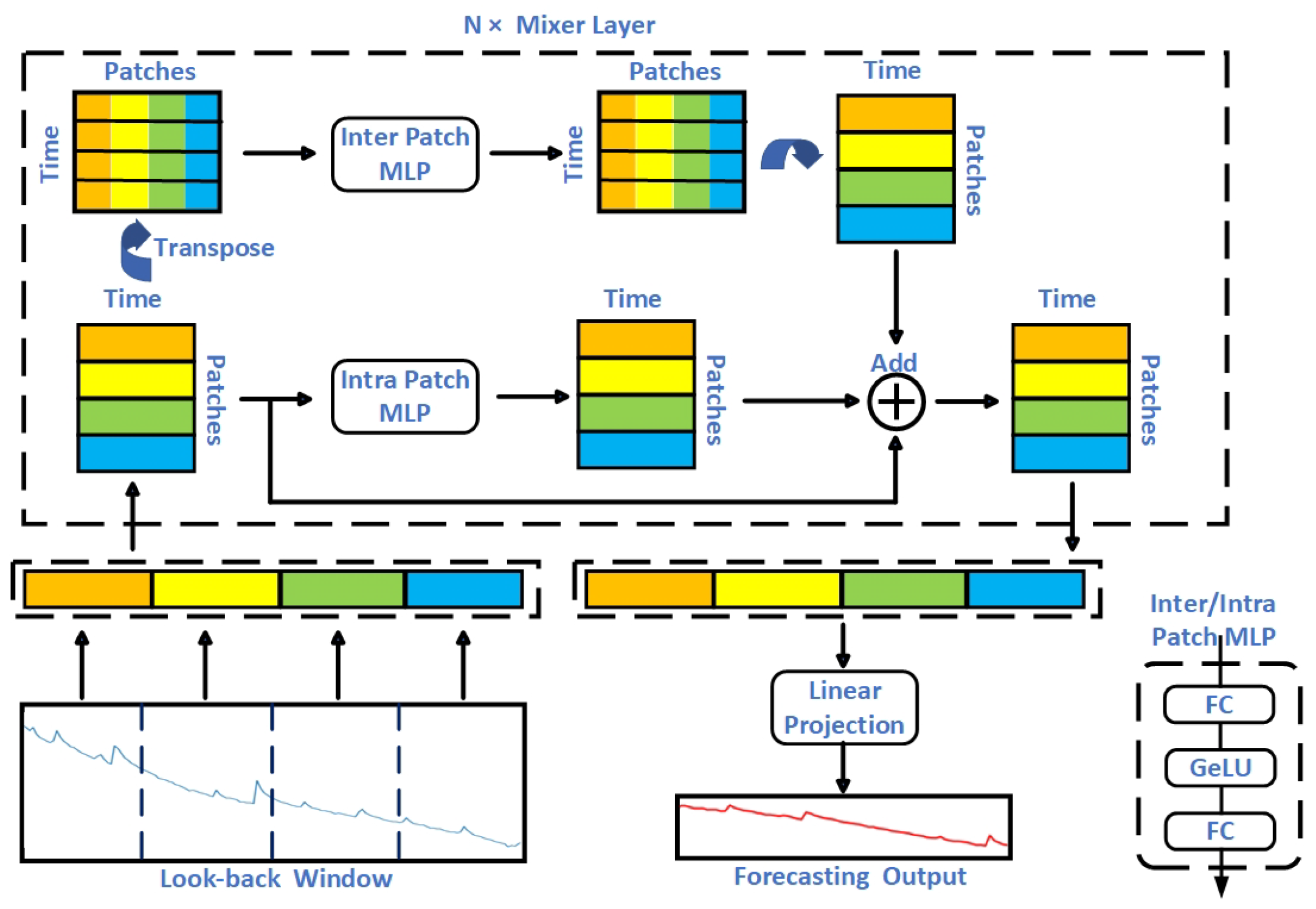
Figure 1. Intra–Inter-Patch Mixing architecture for battery remaining useful life prediction.
Energies 17 03553 g001
Figure 2. Block diagram of the data processing procedure.
Energies 17 03553 g002
Figure 3. Prediction of battery life.
Energies 17 03553 g003
Figure 4. Prediction of battery life with dual-head MLP.
Energies 17 03553 g004
Table 1. Hyper-parameter summary.
Hyper-ParameterRange of Values
Patch size{2, 4, 8}
Learning rate{0.0001, 0.0005, 0.001}
Dropout{0.05, 0.1, 0.2}
Length of patch{2, 4, 8}
# of mixer blocks{1, 2, 3, 4}
# of principal features{1,2,4,6,8,10,12,14,16}
Table 2. Performance of methods on the NASA PCoE battery dataset.
MethodsMAE (Ah)RMSE (Ah)MAPE (%)ARE (%)
Transformer0.0550.0733.6979.589
Informer0.0490.0633.2814.110
MLP0.0500.0663.4026.393
DLinear0.0410.0522.7323.196
IIP-Mixer0.0370.0482.4801.370
Table 3. Evaluation results on the NASA PCoE battery dataset.
MethodsMAE(Ah)RMSE(Ah)ARE
LSTM [42]0.0830.0910.265
Dual-LSTM [41]0.0820.0880.256
GRU [40]0.0810.0920.304
DeTransformer [13]0.0710.0800.225
IIP-Mixer (ours)0.0370.0480.014
Table 4. L-related computation statistics of each layer.
MethodsTrainingTesting
TimeMemoryStep
Transformer O ( L 2 ) O ( L 2 ) L
Informer O ( L log L ) O ( L log L ) 1
MLP O ( L 2 ) O ( L 2 ) 1
DLinear O ( L ) O ( L ) 1
IIP-Mixer O ( L ) O ( L ) 1
Table 5. Ablation study of dual-head MLP.
MethodsMAE (Ah)RMSE (Ah)MAPE (%)ARE (%)
w/o inter0.0810.0955.44334.703
w/o intra0.0440.0552.9405.023
IIP-Mixer0.0370.0482.4801.370
Table 6. Comparison of serial and parallel heads.
MethodsMAE (Ah)RMSE (Ah)MAPE (%)ARE (%)
Serial heads
(inter-first)
0.0630.0764.25815.068
Serial heads
(intra-first)
0.0450.0563.0324.110
Parallel heads0.0370.0482.4801.370
Table 7. Comparison of loss functions with weighting vs. w/o weighting.
MethodsMAE (Ah)RMSE (Ah)MAPE (%)ARE (%)
w/o weighting0.0390.0492.5621.370
With weighting0.0370.0482.4801.370
Table 8. Comparison of time series: univariate vs. multivariate.
MethodsMAE (Ah)RMSE (Ah)MAPE (%)ARE (%)
Univariate0.0420.0542.8223.653
Multivariate
(full)
0.0520.0643.5107.306
Multivariate
(principal)
0.0370.0482.4801.370
Disclaimer/Publisher’s Note: The statements, opinions and data contained in all publications are solely those of the individual author(s) and contributor(s) and not of MDPI and/or the editor(s). MDPI and/or the editor(s) disclaim responsibility for any injury to people or property resulting from any ideas, methods, instructions or products referred to in the content.