Article

Predictive Modeling of Solar PV Panel Operating Temperature over Water Bodies: Comparative Performance Analysis with Ground-Mounted Installations

by
Karmendra Kumar Agrawal
1,
Shibani Khanra Jha
1,*,
Ravi Kant Mittal
1,
Ajit Pratap Singh
1,
Sanjay Vashishtha
2,
Saurabh Gupta
3 and
Manoj Kumar Soni
4
1
Department of Civil Engineering, Birla Institute of Technology & Science, Pilani 333031, Rajasthan, India
2
Firstgreen Consulting Pvt Ltd., Gurgaon 122002, Haryana, India
3
Saub Consulting, Jaipur 302015, Rajasthan, India
4
Department of Mechanical Engineering, Birla Institute of Technology & Science, Pilani 333031, Rajasthan, India
*
Author to whom correspondence should be addressed.
Energies 2024, 17(14), 3489; https://doi.org/10.3390/en17143489
Submission received: 27 May 2024 / Revised: 19 June 2024 / Accepted: 9 July 2024 / Published: 16 July 2024
(This article belongs to the Topic Solar Thermal Energy and Photovoltaic Systems, 2nd Volume)

Abstract

:
Solar panel efficiency is significantly influenced by its operating temperature. Recent advancements in emerging renewable energy alternatives have enabled photovoltaic (PV) module installation over water bodies, leveraging their increased efficiency and associated benefits. This paper examines the operational performance of solar panels placed over water bodies, comparing them to ground-mounted solar PV installations. Regression models for panel temperature are developed based on experimental setups at BITS Pilani, India. Developed regression models, including linear, quadratic, and exponential, are utilized to predict the operating temperature of solar PV installations above water bodies. These models incorporated parameters such as ambient temperature, solar insolation, wind velocity, water temperature, and humidity. Among these, the one-degree regression models with three parameters outperformed the models with four or five parameters with a prediction error of 5.5 °C. Notably, the study found that the annual energy output estimates from the best model had an error margin of less than 0.2% compared to recorded data. Research indicates that solar PV panels over water bodies produce approximately 2.59% more annual energy output than ground-mounted systems. The newly developed regression models provide a predictive tool for estimating the operating temperature of solar PV installations above water bodies, using only three meteorological parameters: ambient temperature, solar insolation, and wind velocity, for accurate temperature prediction.

1. Introduction

With the ever-increasing demand for energy, depleting reserves of fossil fuels and higher levels of environmental pollution have necessitated looking for alternative energy systems. Solar power is a clean and renewable energy resource available in abundance and free has led to the development of solar photovoltaic (PV) power plants worldwide. While solar PV technology has matured significantly, large-scale installations are increasingly being implemented with ground-mounted systems worldwide. Ground-mounted solar PV installation takes much land, and expanding project sizes necessitates big, contiguous land lots, which can be difficult in many circumstances. Floating solar photovoltaic (FSPV), also referred to as floatovoltaics, can be the most favorable alternative to overcome the shortcomings of the ground-based PV system. Many benefits of floating (water-mounted) PV, such as temperature reduction of PV panels, no cost for land, evaporation reduction, and reduced soiling, etc., were reported by Agrawal et al. (2022), Essak and Ghosh (2022), and Huang et al. (2023) [1,2,3]. It is the panel temperature that plays a very important role in terms of solar panel efficiency. The lower operating temperature leads to a reduced temperature coefficient and increased panel efficiency.
The performance of solar panels is highly dependent on their nominal operating cell temperature. The temperature of PV panels depends on many factors, such as ambient temperature, solar insolation, and wind velocity. These factors are assumed to be influencing factors of panel operating temperature and affect the performance of the PV panel. Hence, it becomes important to predict the operating temperature of PV modules.
Hence, many studies have focused on predicting the operating temperature of PV modules. Schott (1985) and Servant (1985) [4,5] proposed an implicit equation, while Lasnier and Ang (1990), Ross and Smoker (1986), and Mondol et al. (2005) [6,7,8] proposed an explicit equation for module operating temperature using meteorological parameters. Coskun et al. (2016) [9] used an artificial neural network to predict PV module operating temperature. Skoplaki and Polyvos (2009) and Skoplaki et al. (2008) [10,11] developed an equation for predicting module operating temperature, showing high function error for wind speed below one m/s. Muzathik et al. (2014) [12] used simple correlation, while Risser and Fuentes (1984) [13] used linear regression to predict PV module operating temperature. Chenni et al. (2007), Kurtz et al. (2009), King (1997), and Akyuz et al. (2012) [14,15,16,17] developed a PV module operating temperature prediction model utilizing three meteorological parameters: solar insolation, ambient temperature, and wind velocity. Almaktar et al. (2013) [18] proposed a module operating temperature model for the tropical region, using only ambient temperature, while Kalogirou (2013) and Irodionov et al. (1989) [19,20] developed the model using ambient temperature and solar insolation to predict module operating temperature. Mora Segado et al. (2015) [21] developed a prediction model for PV modules of different technologies under the climatic conditions of southern Spain using meteorological parameters. Kaplani and Kaplanis (2020) [22] developed a module operating temperature model based on the energy balance equation for all environmental conditions.
Koehl et al. (2011) [23] proposed a Realistic Nominal Module Temperature (ROMT) based on observed field data, whereas Faiman (2008) [24] provided a modified HWB equation to predict the module temperature. Barry et al. (2020) [25] developed a dynamic model of photovoltaic module temperature as a function of atmospheric conditions. Du Y. et al. (2016) [26] developed a theoretical model, while Duffie and Beckman (2006) [27] proposed an equation based on Nominal Operating Cell Temperature (NOCT), Sohani and Sayyaadi (2020) [28] employed genetic programming for predicting solar PV panel temperature. All these models utilize meteorological parameters (solar insolation, ambient temperature, and wind velocity) to predict module temperature. Evans and Florschuetz (1978), Evans (1981), and Notton et al. (2005) [29,30,31] equations give the panel efficiency. Nordmann and Clavadetscher (2003) [32] compared the performance of grid-connected and stand-alone PV systems from 5 countries of different geographic locations. The effect of elevated cell temperature on the annual performance of different mounting namely freestanding, roof-mounted, and integrated PV facades, was studied. All the studies focused on assessing the operating performance of PV modules on ground-mounted solar installation. However, limited work has been performed to predict the operating performance of PV panels over water bodies. Kamuyu et al. (2018) and Tina et al. (2021) [33,34] have developed floating solar PV installation models. Kamuyu et al. (2018) [33] developed the regression model for the Korean region based on the experimental data with meteorological parameters (wind speed, ambient temperature, water temperature, and solar insolation). Tina et al. (2021) [34] developed and validated mathematical models for estimating the performance of bifacial and mono-facial PV modules installed on water surfaces in Catania, Italy. The above studies on performance evaluation of solar PV installation over water bodies have focused on module temperature aspects.
Despite multiple studies conducted for predicting PV module operating temperature under different weather conditions on ground-mounted installations, limited studies were reported for predicting the solar panel operating temperature on water bodies under different weather conditions. This study aims to develop an experimental-based regression model for evaluating the operating temperature of PV panels installed over water bodies operating under different weather conditions. Based on the literature review and subsequent research gap, an attempt has been made to bridge the gap by investigating the following objectives:
  • Identify the influencing factors and performance measures of Floating and ground-mounted solar PV installation;
  • Develop mathematical Models by application of regression analysis with varying parameters;
  • Apply Regression Model Analysis to predict the operating temperature of floating solar PV installation.

2. Existing Module Operating Temperature and Performance Models

The solar energy absorbed by a module is partly converted into electricity, and the balance is converted into thermal energy. Thermal energy increases the cell’s temperature if thermal energy is not dissipated properly. The maximum power point efficiency of a module depends on cell temperature, which can be expressed by Equation (1) (Florschuetz, 1979) [35]:
η m p = η m p . r e f + μ η , m p T c T c , r e f
where η m p is the maximum power point efficiency of the module and μ η , m p is the maximum power point efficiency temperature coefficient. Tc is cell temperature and η m p . r e f and T c , r e f are the reference maximum power point efficiency and reference cell temp i.e., NOCT, conditions respectively. Energy balance on a unit area of the module, cooling by losses to the surroundings, is given by Equation (2) Evans and Florschuetz (1978) [29]:
τ α G T = η c G T + U L T c T a
where τ α is the effective transmittance-absorption product when multiplied by the incident radiation yields absorbed energy and η c is module efficiency to convert incident radiation into electrical energy. The loss coefficient UL includes the losses by convection and radiation from top and bottom and by conduction through the mounting framework to ambient temperature T a . G T is the incident solar insolation on the plane of the module, and Tc is the cell temperature.
Module temperature plays an important role in maximum power point efficiency; therefore, estimation of panel temperature is the prime objective. Various models for PV panel temperature prediction were developed by various authors and are shown in Table 1.
These models can be categorized as linear regression, non-linear regression, and exponential regression. The most widely used ground-mounted PV panel temperature prediction model presented by King et al. (2004) [39] is the exponential regression model. The original general expression for module temperature is given by Equation (3):
T m o d   = T a + G T e a + b w
where G T is solar irradiance incident on module surface ( W / m 2 ), and ‘ a ’ is a dimensionless coefficient establishing the upper limit for module temperature at low wind speeds and high solar irradiance, while ‘ b ’ (s/m) describes cooling by the wind and w wind speed (m/s) measured at 10 m height. These empirically determined coefficients are representative of different module types and mounting configurations.
The above-stated models in Table 1, except Kamuyu et al. (2018) [33] model, and models available in the literature were developed for ground-mounted PV installation, so they could not be utilized to predict module temperature above water bodies. Kamuyu et al. (2018) [33] suggested two linear regression models, namely Tm1 and Tm2, for predicting module temperature mounted over water for floating solar PV installations. Model Tm1 was developed considering meteorological parameters ambient temperature, wind speed, and solar irradiance while model Tm2 was developed by considering water temperature as an additional parameter in addition to parameters of model Tm1. The module operating temperature models Tm1 and Tm2 are given in Equations (4) and (5), respectively:
Tm1 = 2.0458 + 0.9458Ta + 0.0215 GT − 1.2376Vw
Tm2 = 1.8081 + 0.9282Ta + 0.021GT − 1.2210Vw + 0.0246Tw
where Ta is the ambient temperature in °C, GT solar irradiance in W/m2, Vw wind speed in m/s, and Tw is the water temperature in °C.
These empirical formulations have been developed for the Korean region which will not fetch results with the same accuracy for other regions. So, these models need to be checked and corrected for adoption in this region based on the experimental results. To develop temperature prediction models for floating solar in Indian conditions, an experimental setup was established at the Birla Institute of Technology and Science (BITS) Pilani, Pilani campus, India; data were collected, and predictive models were developed.

3. Experimental Setup in the Field

The experimental setup has been installed at BITS, Pilani (India), to assess the operating performance of solar panels over water bodies vis-à-vis ground-mounted installations. The experiment was carried out at Birla Institute of Technology and Science (BITS), Pilani, Rajasthan, India, at Latitude 28° 21′34.1316″ N, Longitude 75° 35′17.2896″ E, at an elevation of 299 m above mean sea level. Four multi-crystalline Si modules with 72 cells were chosen for the present study. The module’s current and voltage temperature coefficients, as provided by the manufacturer, are 14.6 micro-A/cm2/ and −2.10 mV/cell/ , respectively. The nominal power of each module is 320 Wp with a module efficiency of 16.1%. The module and cell areas are 1.9345 m2 and 243.36 cm2, respectively. The experimental test rig consists of four photovoltaic modules. Three PV modules were installed at different heights above the water surface, namely, 300 mm, 500 mm, and 1000 mm, and one ground mounted. The PV modules were facing south direction, having a fixed tilt of 25°, almost the same as the latitude of Pilani. The Pyranometer, from Kipps and Zones CMP 11, was installed on the PV plane to record global solar radiation in the PV plane. The experimental design is shown in Figure 1, and actual experimental pictures are shown in Figure 2.
Temperature sensors Pt100 were installed at the back of panels to monitor the panel’s temperature. The data were recorded automatically through the data logger Data taker DT85 for one year with 15-minute and 1-minute intervals. The ambient temperatures were monitored at 2 m height via the AARHT1K-4-20 PT100 RTD sensor (Manufacturer Aashay Instruments, Pune, Maharashtra, India), and the humidity was monitored through the WS08P sensor. The wind velocity and direction were monitored by digital anemometer AA-WS-50_4-20 and AA-WD-360_4-20, respectively. The wind speed and direction were measured at 2 m height. The water temperature below each panel was also recorded via RTD Pt100. The area around the experimental setup was free from any obstructions for wind as well as solar insolation. Figure 1 shows the setup at the site. The installation was performed over the ground where natural conditions prevail. All data points where the solar radiation was negative and where there were unusual readings (>1500 in solar radiation) were removed. For the simplicity of the Model and its widespread coverage, three key parameters were used: solar radiation, ambient temperature, and wind speed. A panel height of 500 mm above the water surface has been obtained as the best height for performance (Agrawal et al., 2024) [41]. Therefore, data from the panel with a 500 mm height above the water surface are used for the current analysis and model development.
The data was collected for an entire year, and different regression models were developed. Linear, quadratic, and exponential regression models were developed to evaluate the performance of solar PV over water bodies, and a comparative study among all models for seasonal variation and annual variation was carried out. The impact of variations of different meteorological parameters (such as wind speed, ambient temperature, water temperature, humidity, and solar insolation) has also been assessed on the accuracy of the operating temperature of panels.

4. Modeling Procedure

The experimental setup was utilized to collect data for modeling the temperature of the PV modules. These experiments aimed to create a model that would predict the temperature of photovoltaic (PV) panels based on specific meteorological parameters. The experimental set-up, which has the test rig consisting of PV modules, served as the basis for this. The information included a variety of parameters, including the air/ambient temperature (Ta), the water temperature (Tw), the solar insolation (GT), the wind speed (v), and the relative humidity (Rh). Though the test rig consisted of four solar panels, however, the modelling is performed based on ground-mounted solar panels and a comparison with the best performing floating solar panel at 500 mm height over the water body.

4.1. Exponential Model Using Experimental Data

In the first experiment, a set of coefficients in Equation (3) were obtained for predicting floating PV panel temperature. The coefficients were determined for the FSPV panel as well as the ground-mounted panel with the original three meteorological parameters: solar radiation, ambient temperature, and wind speed.
Focusing on solar radiation, water temperature, and wind speed, the second experiment aimed to estimate the panel temperature in response to meteorological factors. In this investigation, alternate models were created using water temperature (Tw) instead of ambient temperature (Ta) and then new coefficients were derived. A fitting exercise using the current data to find the coefficients of the exponential regression equation (3) and the R-square values resulting from those coefficients are given in Table 1. These findings were analyzed, comparing predicted and actual temperatures for both ground-mounted and water-mounted panels and evaluating the necessity of adapting the current empirical models to local conditions.
Equation (6) shown below, referred to as model GM1 in Table 1, is developed for ground-mounted panels, but it is used beyond ground-mounted panels to forecast temperatures for panels mounted above water. A greater correlation than ground-mounted panels was demonstrated by the resulting R2 value of 0.848, which suggests a more precise forecast of panel temperatures over water.
T m o d   = T a + G T e 3.085 0.032 v
The modified Equation (7), named the F1 model, with a new coefficient for the water mounting panel is developed considering the original variables, namely ambient temperature, solar insolation, and wind velocity.
T m o d   = T a + G T e 3.359 0.022 v
The model was further modified by substituting water temperature for ambient temperature in the original equation and Equation (8), named the F2 model, was developed for water-mounted panels.
T m o d   = T a + G T e 2.998 0.025 v
The R2 values for models F1 and F2 were obtained as 0.955 and 0.94, respectively, as detailed in Table 2.

4.2. Linear and Quadratic Models Using Experimental Data

The operating temperatures of solar panels are predicted in this section by a thorough investigation of regression modeling, with a special emphasis on water-mounted panels. The newly determined coefficients incorporate ambient temperature into the model; the exponential equation is reliable in estimating the temperature of these panels. However, it is better suited for analysis with fewer meteorological parameters because it only includes three variables: sun insolation, wind speed, and ambient temperature.
The exponential equations, despite being straightforward and useful, ignore the importance of humidity, a vital element that could significantly impact panel temperatures, particularly diurnal and seasonal variations like early in the morning and during the rainy season. Given that floating solar panels are mounted above bodies of water, it is assumed significant to take humidity into account. In the present study regression model with the inclusion of humidity and water temperature was planned and developed, both linear and non-linear regression models, to evaluate this impact on panel temperature prediction. With the Solar PV Panel Temperature (in degrees Celsius) as the dependent variable (target variable), the regression analysis included a wide range of independent variables, namely Ambient Temperature (degrees Celsius), Water Temperature (degrees Celsius), Solar Insolation (W/m2), Wind Speed (km/h), and Humidity (%). Models were developed considering three variables (ambient temperature, solar insolation, and wind speed), four variables (adding water temperature), and five variables (adding humidity) in the regression analysis. Additionally, to test the non-linearity, the quadratic models were also developed. Table 3 displays various regression models, R-square values, model equations, variables, and model nomenclatures that go with them. A one-year meteorological and panel temperature data with a 15-min interval is used to test each model. All models performed well in terms of R2 values greater than 0.9.
A-linear regression models F3, F4, and F5 are represented in Equations (9)–(11), respectively.
T m o d = 0.337 + 0.034 G T 0.056 v + 0.995 T a
T m o d = 8.736 + 0.927 T w + 0.043 G T 0.027 v 0.105 R h .
T m o d = 6.833 0.491 T w + 0.03 G T 0.068 v + 1.526 T a + 0.08 R h
B-Quadratic Linear Regression models F6, F7, and F8 are represented in Equations (12)–(14) respectively.
T m o d = 3.116 + 0.044 G T + 0.71 v + 1.156 T a 0.001 G T v 0.104 v 2 + 0.003 v T a 0.004 T a 2
T m o d = 3.961 + 1.008 T w + 0.082 G T + 1.852 v 0.153 R h 0.002 T w 2 0.015 v T w + 0.003 T w R h 0.002 v G T 0.129 v 2 0.009 v R h + 0.001 R h 2
T m o d = 9.506 0.39 T w + 0.044 G T + 1.038 v + 1.487 T a + 0.116 R h + 0.029 T w 2 + 0.001 T w G T 0.015 v T w 0.053 T w T a + 0.002 R h T w 0.001 v G T 0.001 T a G T 0.094 v 2 + 0.008 v T a 0.004 v R h 0.001 T a R h + 0.023 T a 2
where, Tw = Water temperature in °C, GT = Solar insolation in W/m2, Ta = Ambient temperature in °C, v = Wind velocity in km/h, Rh = Relative humidity in %.

5. Testing the Models for Seasonal Adequacy

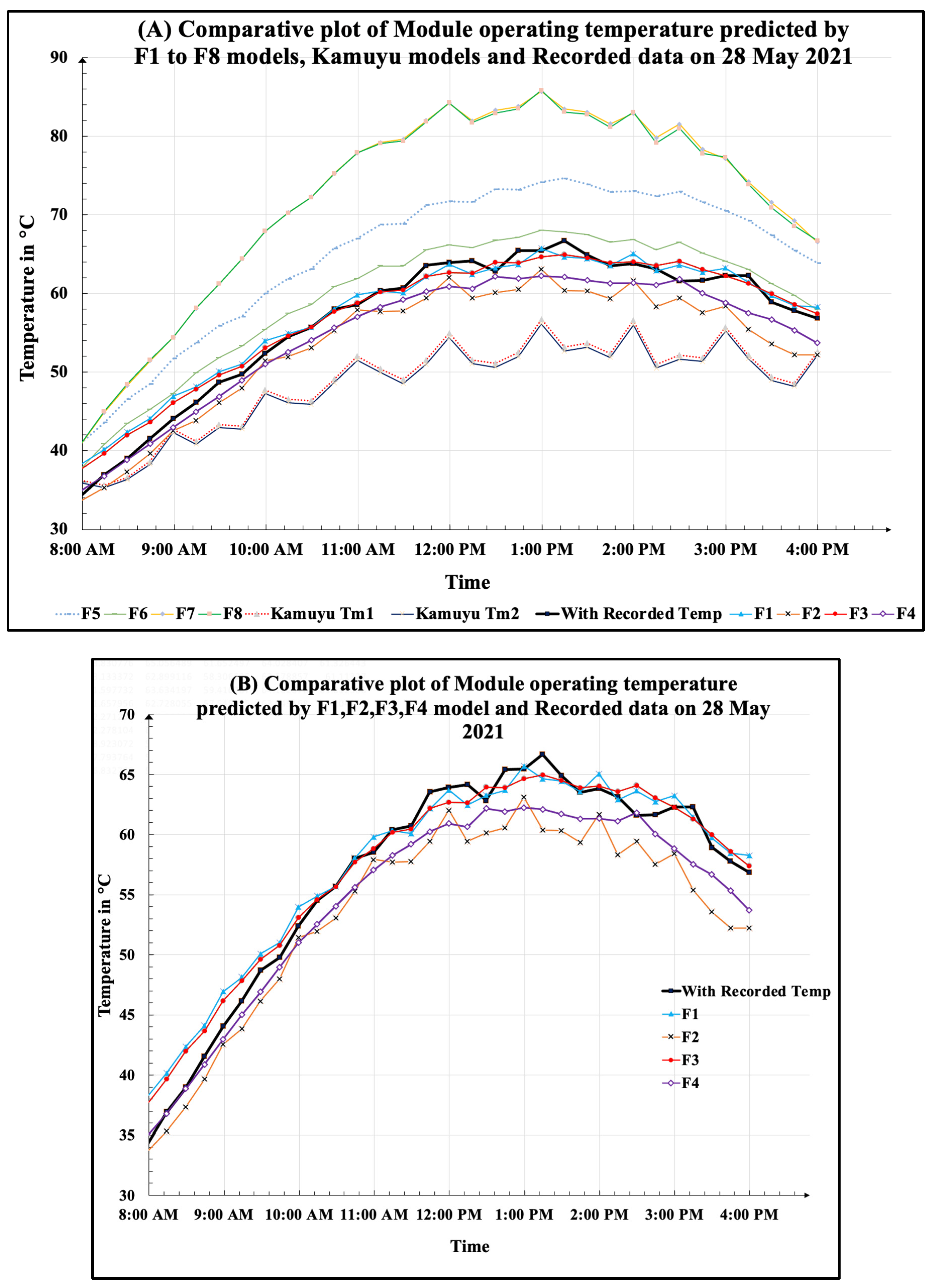
The suitability of each model developed above was examined during all seasons. These models were tested for estimating the temperature of a panel mounted 500 mm above the water surface. Figure 3 shows the temperature forecasts from all eight models (F1 to F8) and Kamuyu et al. (2018) [33] models (Tm1 and Tm2) and the recorded panel temperature for a typical day in May, with maximum solar insolation. The root mean square error (RMSE) of each model is estimated for the annual dataset and it is presented below in Table 4.
With a maximum error of 5.5 degrees and a minimum error of 1.67 degrees, Model F3 was found to be the best model in terms of root mean square error (RMSE). This strong performance is noteworthy, especially because several linear, non-linear, and exponential models considering additional parameters such as water temperature and humidity were developed. But, in the analysis, the simplest model with a three-parameter, namely ambient temperature, solar insolation, and wind speed, proved to be more useful. The models with fewer parameters outperformed those that took extra factors like humidity and water temperature into account.

5.1. Seasonal Evaluation and Model Identification for Best Performance

The three main seasons experienced in India—summer (March to June), monsoon (July to September), and winter (October to February)—were used to subject the regression models to extensive testing. Table 5 shows how the models’ performance varied with the seasons. For example, the correlation coefficient varied from 0.87 for F5 in the summer to 0.98 for F1 in the winter, while the R2 value ranged from 0.75 for F5 to 0.95 for F1, with the lowest and highest values again occurring in the summer and winter, respectively. With a maximum inaccuracy as reflected in terms of RMSE in summer of 7.3 degrees and the lowest error in winter of 2.74 degrees, Model F3 consistently shows the highest performance.
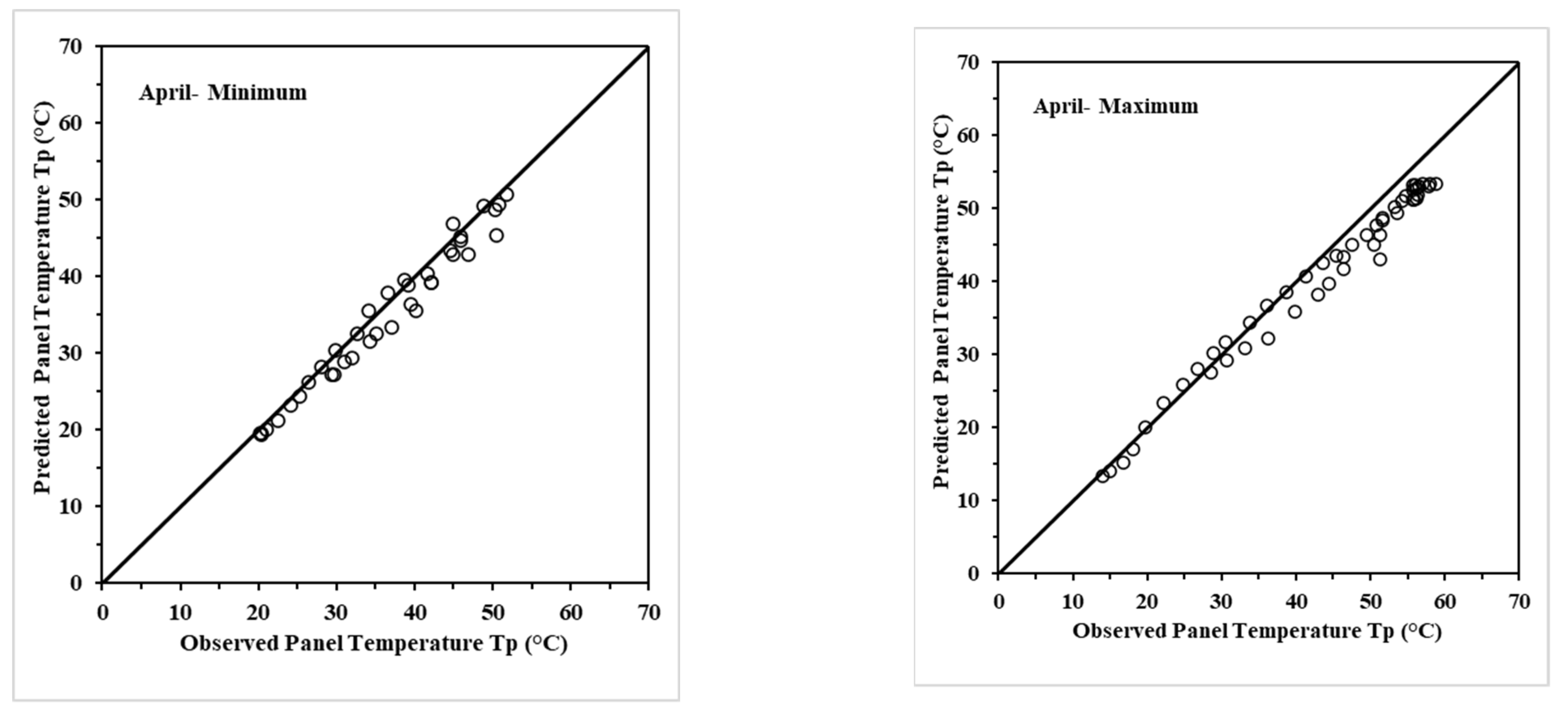
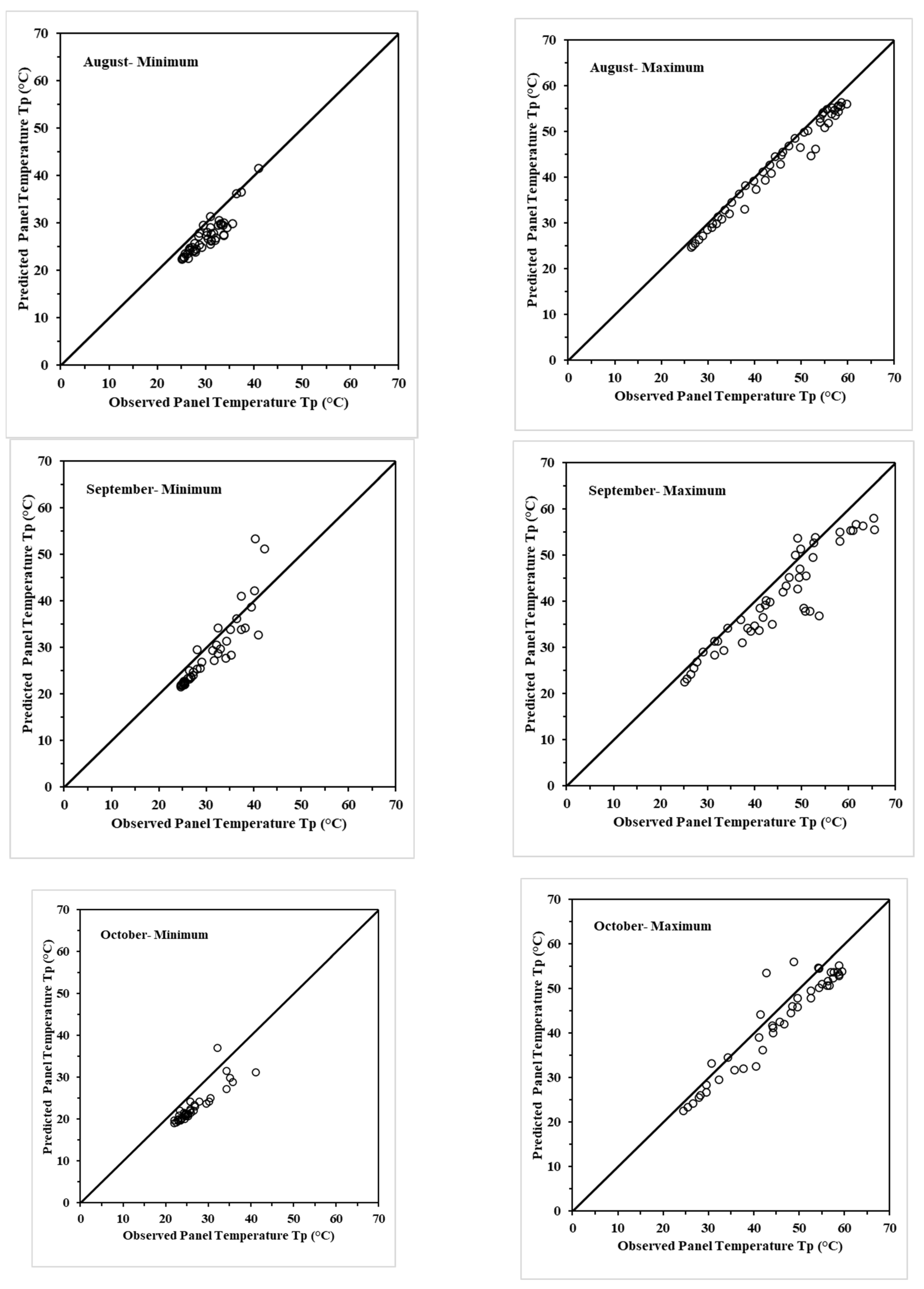
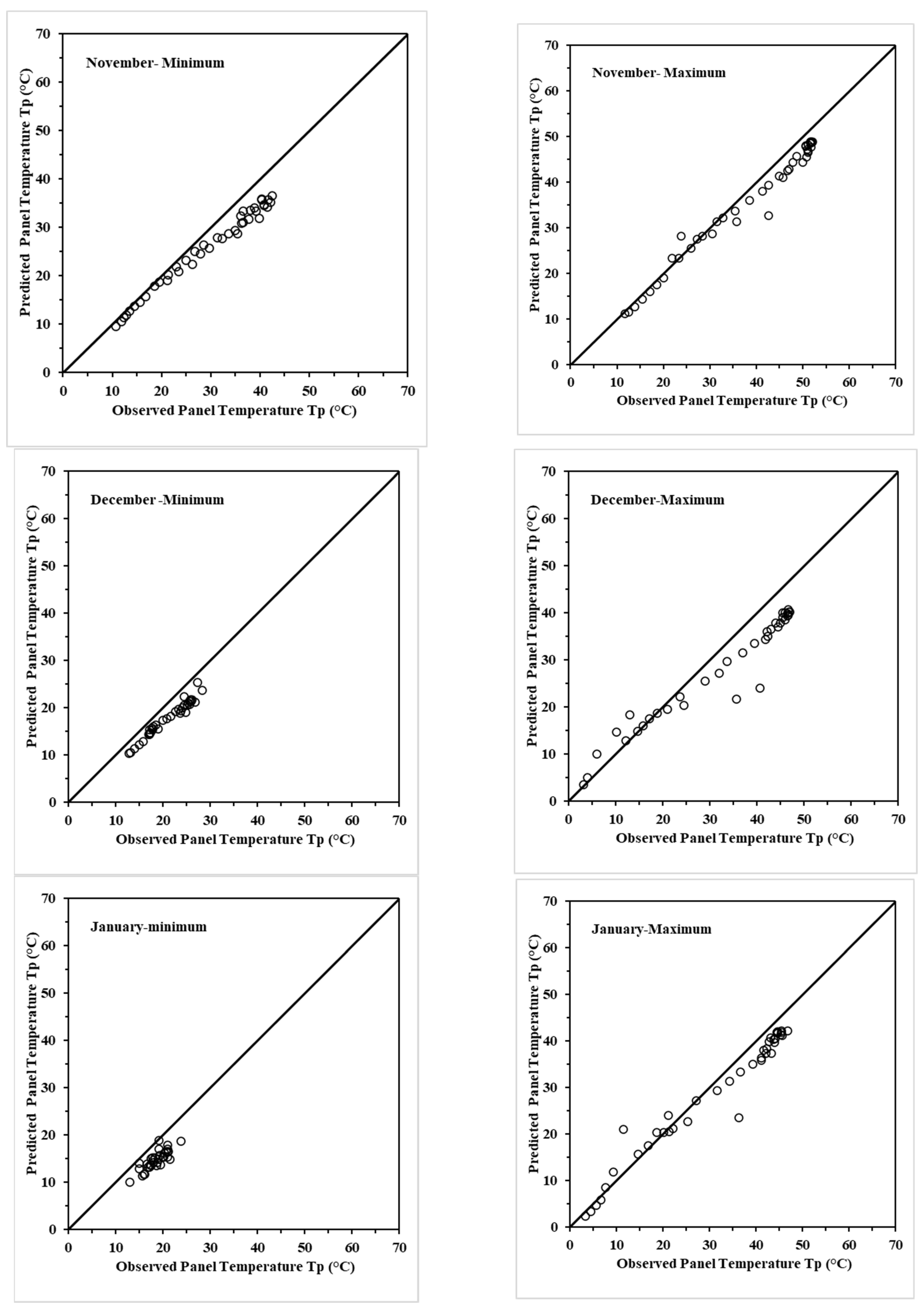
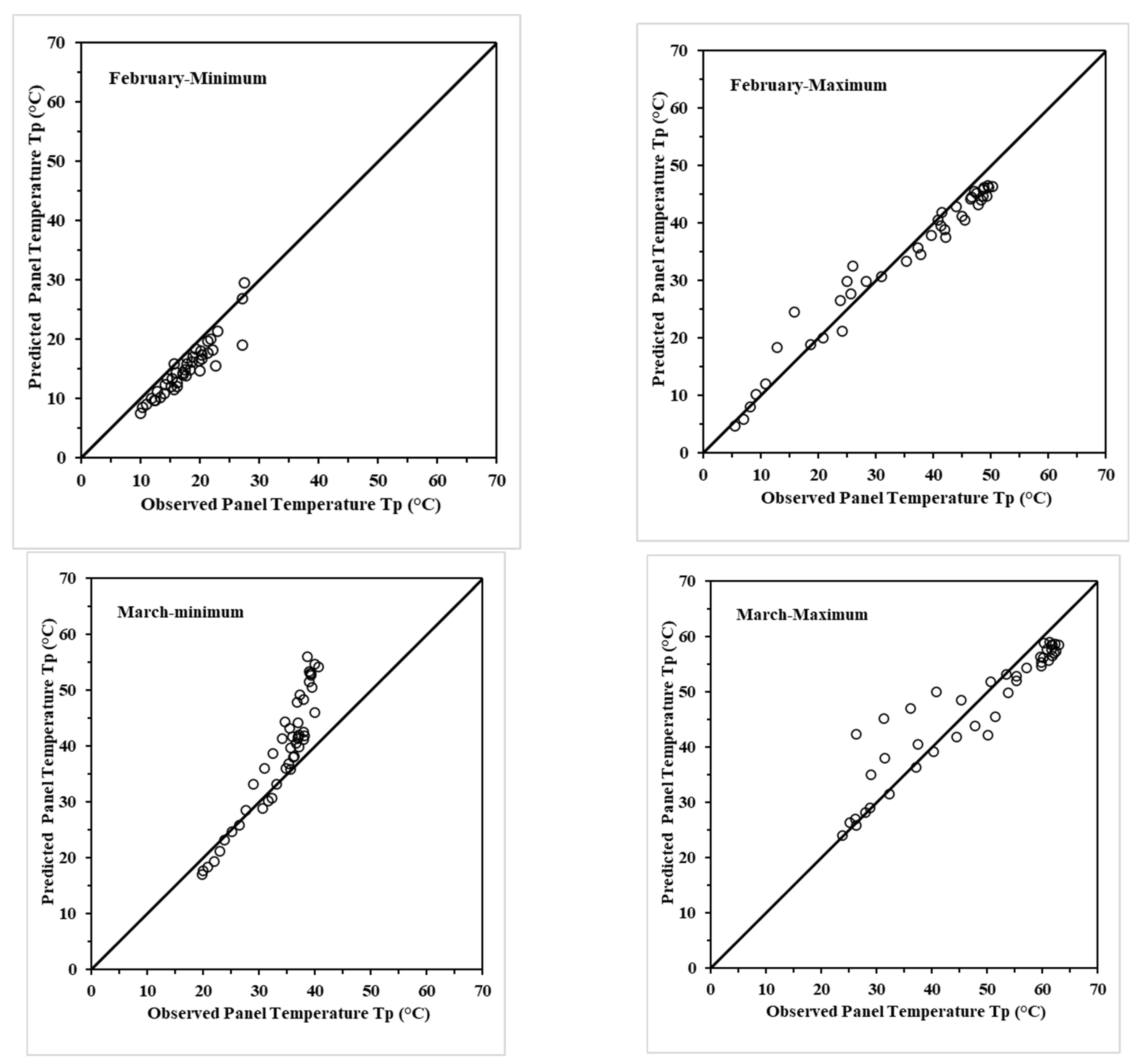
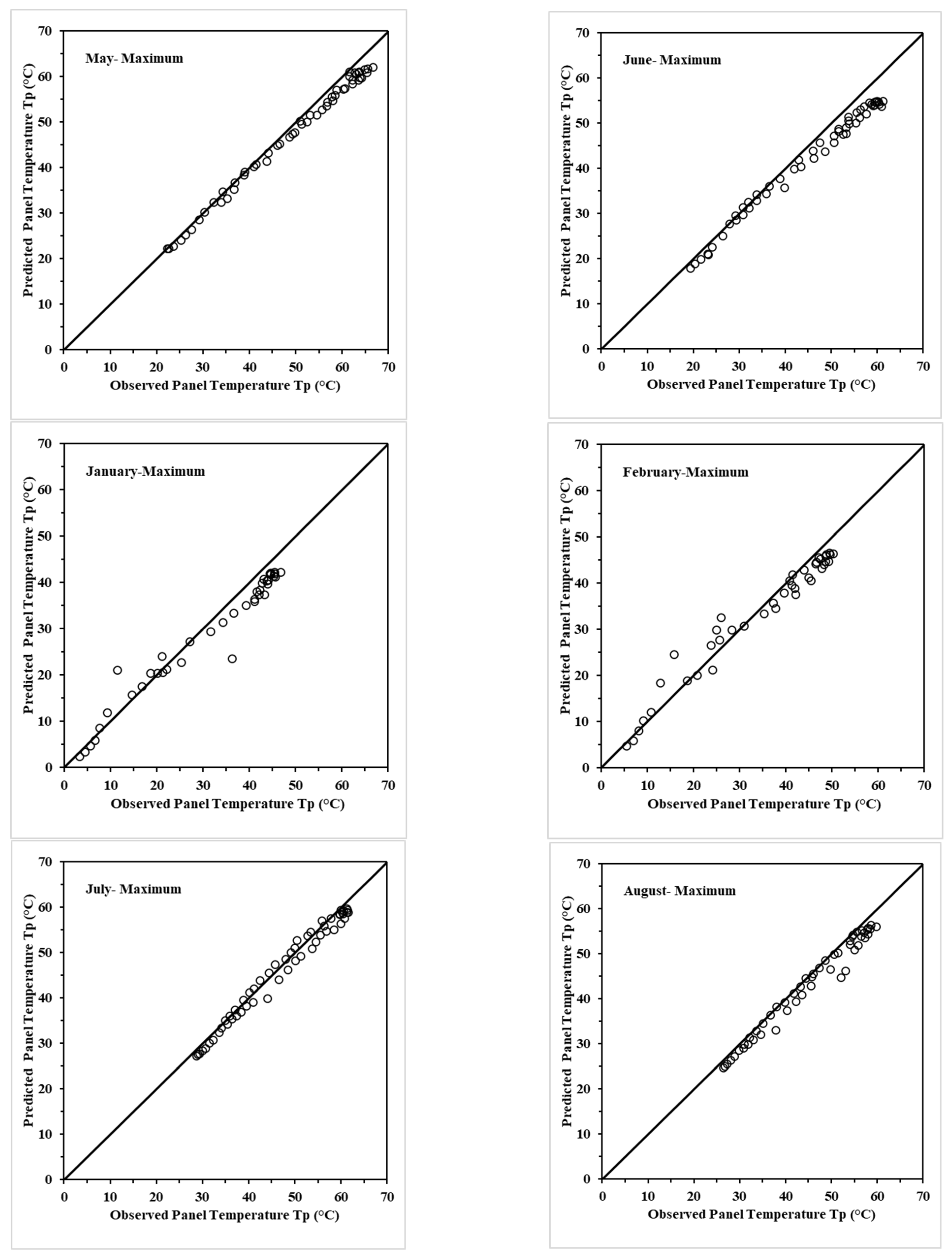
The predictive model takes into account regional climatic trends because of the seasonal fluctuations in model performance. A well-balanced model that can accommodate a variety of climatic conditions throughout the year is important, and Model F3, which consistently outperformed all other models across all seasons, is a good example. The plots of the predicted panel temperature to recorded panel temperature for maximum value from Model F3 for summer (May and June), winter (January and February), and monsoon (July and August) are shown in Figure 4. Additionally, the plots of predicted panel temperature to recorded panel temperature from Model F3 for the maximum and minimum of all the months of a year are annexed in Appendix A. The plots shown in Figure 4 outline the robustness of model F3; it not only predicts well in all the seasons, but it also captures higher temperatures of 65 degrees with equal precision as lower temperatures of 2 degrees during winters. The high humidity during monsoon is well captured by the model, visible from the plot of monsoon months July and August. The RMSE during summer, winter and monsoon are in proportion to the temperature of the panels. The temperature during summers is as high as 70 degrees while the temperature during winters remains in the range of 45 degrees, so the model is performing equally well in all the seasons. Overall, results highlight the necessity of incorporating seasonal environmental variability into predictive models for solar panel temperature to ensure dependable and accurate energy estimation annually.

5.2. Evaluation of Energy Output from Developed Models

The models were tested for energy estimation to see the impact of error in the prediction of temperature. The power is estimated using Equation (15) given below:
P o w e r = G T × A M × η M r e f 1 β M r e f × T M T r e f
where GT is solar insolation in W/m2, AM = Area of the module in m2, ηMref = module efficiency at NOCT, βMref = power temperature coefficient in %, TM = module temperature in °C and Tref = NOCT temperature 25 °C. For present case module area AM = 1.9345 m2, ηMref = 16.1%, βMref = 0.5% W/°C.
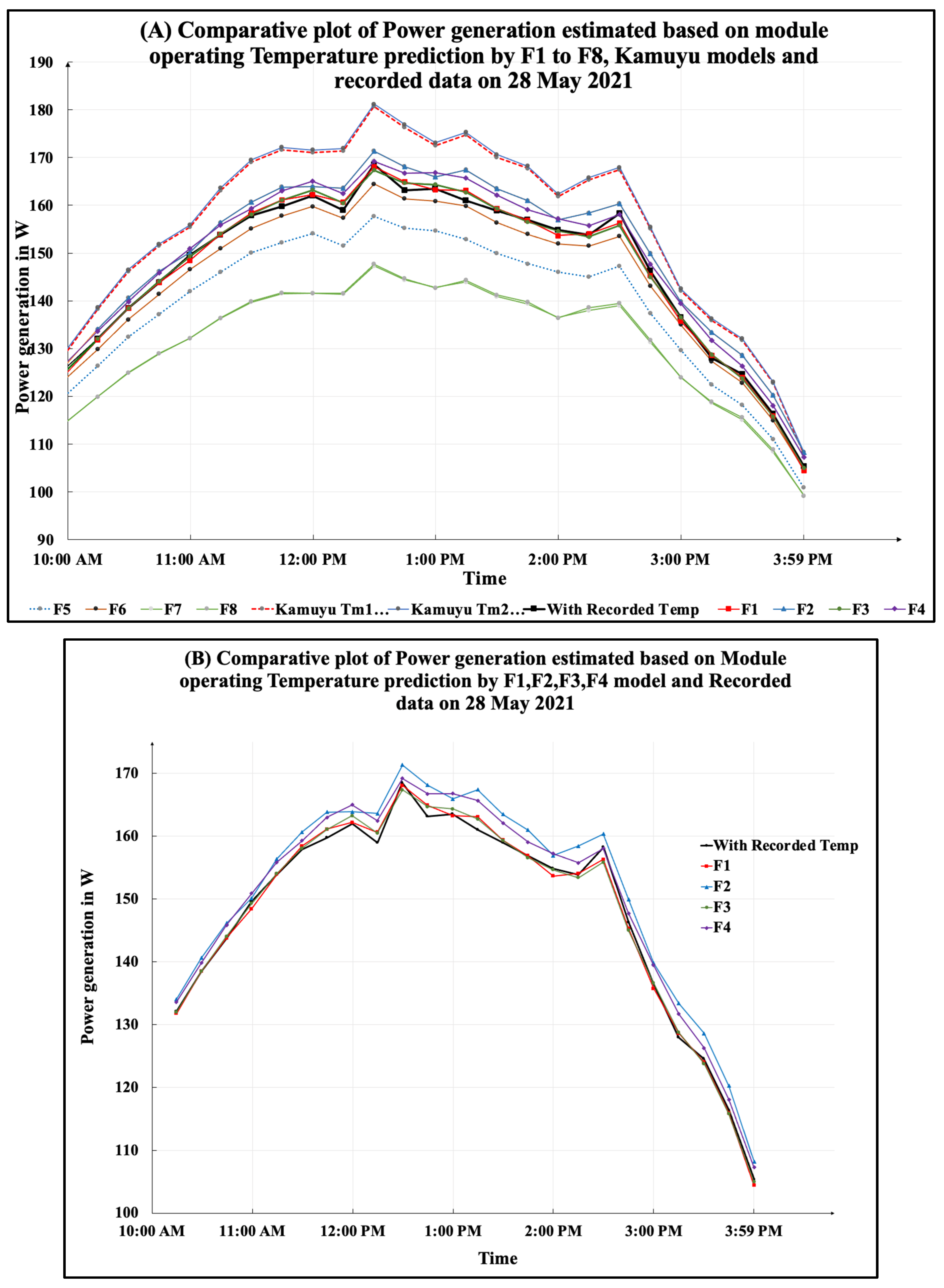
Energy estimations were performed for the highest and lowest solar insolation days on two typical days within each month. This was based on information gathered over 12 months. The estimated energy production was then compared with the temperature data gathered from the modules and the temperature forecasts from the different models, as shown in Table 6. A typical May Day with maximum solar insolation is depicted in Figure 5, along with the expected temperature for that day using data from all eight models. It is clear, as indicated in Table 6 that Model F3 produced an accurate energy estimation. It is interesting to note that both Model F2 and Model F4, which come second in accuracy, consider water temperature rather than ambient temperature. In addition, the model by Kamuyu et al. (2018) [33] for floating PVs’ module operating temperature was used to estimate the energy production. With the Tm1 model, as given in Equation (4), this model’s energy estimation error was 4.10%, while with the Tm2 model given by Equation (5), it was 4.31%. Figure 5 displays the power estimate from recorded panel temperature data, estimates from F1–F8 models, and the models from Kamuyu et al. (2018) [33].

Assessment of Energy Output from Developed Models: Seasonal Variation

Across several seasons, the energy output is also calculated from the module operating temperature by all the models, as shown in Table 7. The model tested for seasonal variation in energy prediction shows a variation of −1.19% in summer to 0.07% in winter for model F1, while model F2 shows a variation of −1.10% in summer to 0.12% in winter. Model F3 is also three parametric using solar insolation, wind velocity, and ambient temperature showing the lowest variation of 0.35 in summer and 0.59 in winter. Model F4 is four parametric using solar insolation, wind velocity, humidity, and water temperature. Model F4 shows a variation of −1.09% in summer to 0.34% in winter. Other models, F5, F6, F7, and F8, vary from −1.49% to −10.44%. These models were developed to observe the effect of humidity, water temperature, and non-linearity. The non-linear regression models do not show any improvement in the prediction, even with all five variables. Thus, the linear models with three variables are the best representative models.
The results of this investigation showed that the most accurate predictions were made using three-parameter models that included solar insolation, wind speed, and either ambient or water temperature. The prediction was worsened by two-degree regression models, and the prediction was not improved by adding all five parameters. Additionally, the impact of water temperature was not much stronger than that of ambient temperature. These findings help to improve the design and operation of solar energy systems by offering helpful insights into the critical variables determining energy output.

6. PV Panel Operating Temperature Variations: Comparison of Floating vs. Ground-Mounted PV Panels

The goal of the comparative study is to look at how the operating temperatures of floating and ground-mounted photovoltaic (PV) panels differ. The temperature measurements of both panel types across several seasons must be analyzed in order to fully comprehend the significance of these variances. The yearly maximum, lowest, and average operating temperatures for solar panels that are ground-mounted and afloat are shown in Table 8. Despite the numbers mentioned above, it is not immediately clear how these temperature changes affect energy generation. Equation (15) was used to predict energy output for both types of panels while taking the potential impact of temperature on energy generation into account.
The energy output was then calculated using the reported temperatures for both types of panels. Two typical days of maximum and minimum solar insolation each month were used to determine the energy production. Data collected over a year is used to obtain these results, which are provided in Table 9. The projected energy generation for each month is shown graphically in Figure 6. The findings demonstrate that floating solar panels provide 2.59% more energy generation yearly than PV systems that are installed on the ground. This finding implies that ground-mounted PV panels maintain an average temperature that is roughly six degrees higher than floating PV panels. Due to the substantial lowering of temperature, floating PV systems outperform ground-mounted ones in terms of energy output.

7. Conclusions

The study found that the average operating temperature of modules mounted over the ground is six degrees higher than those mounted over water. Regression analysis was used to develop and validate models for predicting the operating temperature of floating solar PV modules. The models incorporated various meteorological parameters, including ambient temperature, solar insolation, wind velocity, water temperature, and humidity. The study concluded that
  • The three parametric models, F1 and F3, which utilized ambient temperature, solar insolation, and wind velocity, predicted panel operating temperature the best, with a maximum root mean square error (RMSE) of 5.64 °C and 5.50 °C, respectively. On the other hand, three parametric models replacing ambient temperature with water temperature, F2 and F4, predicted panel operating temperature less accurately, with a maximum RMSE of 8.26 °C and 9.43 °C, respectively;
  • The study also found that the one-degree regression model with all five parameters did not add to the accuracy of the prediction model. However, the two-degree regression models were complex, with an RMSE of more than 20 °C;
  • Finally, the study found that the best model is F3, which can be used to predict the operating temperature of the panel and power estimates, assessing the module’s overall performance;
  • Floating solar PV systems should be preferred to ground-mounted ones due to the lowering of operating temperatures by 6 °C. The study found that floating solar PV installations consistently produced 2.59% more energy than ground-mounted solar PV installations.

Author Contributions

K.K.A.: Conceptualization, Data curation, Formal analysis, Investigation, Writing—original draft; S.K.J.: Conceptualization, Supervision, writing—reviewing of original draft and editing, communicating; R.K.M.: Project administration, Supervision, reviewing; S.V.: Funding support, industrial guidance; A.P.S.: Writing: Supervision of the work; S.G.: Formal analysis; M.K.S.: Resource support. All authors have read and agreed to the published version of the manuscript.

Funding

Experimental setup at BITS, Pilani was supported by a grant from Firstgreens Consulting Pvt Ltd., Gurgaon, Haryana 122002, India.

Data Availability Statement

The sample dataset is available in the manuscript and additional data may be available on request.

Acknowledgments

The authors are sincerely thankful to the Birla Institute of Technology and Science, Pilani, for supporting this research work under the PhD thesis scheme.

Conflicts of Interest

Author Sanjay Vashishtha was employed by the company Firstgreens Consulting Pvt Ltd. Author Saurabh Gupta was employed by the company Saub Consulting. The remaining authors declare that the research was conducted in the absence of any commercial or financial relationships that could be construed as a potential conflict of interest.

Appendix A

Figure A1. Plots of predicted panel temperature vs recorded panel temperature for maximum and minimum by best-performing F3 model.
Energies 17 03489 g0a1aEnergies 17 03489 g0a1bEnergies 17 03489 g0a1cEnergies 17 03489 g0a1dEnergies 17 03489 g0a1e
Table A1. Sample data for maximum insolation day on 18th April 2021.
Date and TimeSolar Panel Temp at Height 50 cm above Water Surface (°C)Wind Speed (km/h)Ambient Temperature (°C)Humidity (%)Solar Radiation (W/m2)Water Temperature (°C)
18/04/21 6:1514.020.0016.7352.142.3319.28
18/04/21 6:3014.960.0017.0152.5813.2219.20
18/04/21 6:4516.720.0017.8153.1422.5319.29
18/04/21 7:0018.150.0019.0853.9339.2119.36
18/04/21 7:1519.750.0021.3954.4462.9919.47
18/04/21 7:3022.150.0023.7453.3092.6919.64
18/04/21 7:4524.730.4625.0551.17126.9519.81
18/04/21 8:0026.840.0025.9149.60164.1120.05
18/04/21 8:1528.921.4326.7648.32203.6820.33
18/04/21 8:3030.492.6326.8746.88247.5520.59
18/04/21 8:4533.862.0828.2446.16287.9520.85
18/04/21 9:0036.100.0028.9944.85327.7021.25
18/04/21 9:1538.702.4929.6843.76367.1621.68
18/04/21 9:3041.312.3830.4442.63407.0822.09
18/04/21 9:4543.672.2531.0541.62442.7822.50
18/04/21 10:0045.430.0031.3540.48459.1222.87
18/04/21 10:1547.532.9731.7439.63498.7223.11
18/04/21 10:3049.502.3332.2839.06520.5623.38
18/04/21 10:4550.902.1332.6638.20547.3223.69
18/04/21 11:0051.660.0032.8237.06569.6323.96
18/04/21 11:1553.313.0133.5736.36598.7924.13
18/04/21 11:3056.271.9033.9035.66620.1924.39
18/04/21 11:4556.462.5933.7934.65638.6624.64
18/04/21 12:0055.780.0133.9633.65651.4324.83
18/04/21 12:1556.482.8034.2332.93658.9725.03
18/04/21 12:3058.772.1434.6132.50658.5525.24
18/04/21 12:4555.804.3034.1431.81668.5025.39
18/04/21 13:0056.070.0034.0631.07667.5725.52
18/04/21 13:1557.053.4035.0030.82649.5925.77
18/04/21 13:3056.273.5634.7130.08637.1625.90
18/04/21 13:4557.793.2635.3229.80629.4926.13
18/04/21 14:0058.030.0135.6329.51627.4426.31
18/04/21 14:1554.273.7634.7829.08585.2526.51
18/04/21 14:3054.833.7235.4428.52588.0526.72
18/04/21 14:4555.903.3835.5628.52570.3726.92
18/04/21 15:0055.770.0036.1227.80545.9527.18
18/04/21 15:1553.594.3135.2427.52523.8527.35
18/04/21 15:3051.653.9835.5327.24488.3127.51
18/04/21 15:4551.343.3335.4226.95334.3027.67
18/04/21 16:0051.310.0035.5426.52424.2927.84
18/04/21 16:1550.432.6835.7526.39382.5728.03
18/04/21 16:3046.352.0235.6726.11332.0828.20
18/04/21 16:4546.431.9635.6626.11286.3028.35
18/04/21 17:0044.510.0035.2425.78236.4028.42
18/04/21 17:1542.900.7735.2625.54192.3128.51
18/04/21 17:3039.931.8434.9225.40136.9928.45
18/04/21 17:4536.271.1933.7924.9760.3828.38
18/04/21 18:0033.160.0033.0025.1140.4528.35
18/04/21 18:1530.690.0731.9825.1223.1028.25
18/04/21 18:3028.510.0030.7825.688.1028.15

References

  1. Agrawal, K.K.; Jha, S.K.; Mittal, R.K.; Vashishtha, S. Assessment of floating solar PV (FSPV) potential and water conservation: Case study on Rajghat Dam in Uttar Pradesh, India. Energy Sustain. Dev. 2022, 66, 287–295. [Google Scholar] [CrossRef]
  2. Essak, L.; Ghosh, A. Floating photovoltaics: A review. Clean Technol. 2022, 4, 752–769. [Google Scholar] [CrossRef]
  3. Huang, G.; Tang, Y.; Chen, X.; Chen, M.; Jiang, Y. A comprehensive review of floating solar plants and potentials for offshore applications. J. Mar. Sci. Eng. 2023, 11, 2064. [Google Scholar] [CrossRef]
  4. Schott, T. Operation temperatures of PV modules: A theoretical and experimental approach. In Proceedings of the Sixth EC Photovoltaic Solar Energy Conference, London, UK, 15–19 April 1985. [Google Scholar]
  5. Servant, J.M. Calculation of the cell temperature for photovoltaic modules from climatic data. In Intersol Eighty Five; Pergamon: Cambridge, UK, 1986; pp. 1640–1643. [Google Scholar]
  6. Lasnier, F.; Ang, T.G. Photovoltaic Engineering Handbook; Adam Hilger: New York, NY, USA, 1990; p. 80. [Google Scholar]
  7. Mondol, J.D.; Yohanis, Y.G.; Smyth, M.; Norton, B. Long-term validated simulation of a building integrated photovoltaic system. Sol. Energy 2005, 78, 163–176. [Google Scholar] [CrossRef]
  8. Ross Jr, R.G.; Smokler, M.I. Flat-Plate Solar Array Project: Final Report: Volume 6, Engineering Sciences and Reliability; Jet Propulsion Lab.: Pasadena, CA, USA, 1986. [Google Scholar]
  9. Coskun, C.; Koçyiğit, N.; Oktay, Z. Estimation of pv module surface temperature using artificial neural networks. Mugla J. Sci. Technol. 2016, 2, 15–18. [Google Scholar] [CrossRef]
  10. Skoplaki, E.; Boudouvis, A.G.; Palyvos, J.A. A simple correlation for the operating temperature of photovoltaic modules of arbitrary mounting. Sol. Energy Mater. Sol. Cells 2008, 92, 1393–1402. [Google Scholar] [CrossRef]
  11. Skoplaki, E.; Palyvos, J.A. Operating temperature of photovoltaic modules: A survey of pertinent correlations. Renew. Energy 2009, 34, 23–29. [Google Scholar] [CrossRef]
  12. Muzathik, A.M. Photovoltaic modules operating temperature estimation using a simple correlation. Int. J. Energy Eng. 2014, 4, 151. [Google Scholar]
  13. Risser, V.V.; Fuentes, M.K. Linear regression analysis of flat-plate photovoltaic system performance data. In Proceedings of the 5th Photovoltaic Solar Energy Conference, Athens, Greece, 17–21 October 1983. [Google Scholar]
  14. Akyuz, E.; Coskun, C.; Oktay, Z.U.H.; Dincer, I. A novel approach for estimation of photovoltaic exergy efficiency. Energy 2012, 44, 1059–1066. [Google Scholar] [CrossRef]
  15. Chenni, R.; Makhlouf, M.; Kerbache, T.; Bouzid, A. A detailed modeling method for photovoltaic cells. Energy 2007, 32, 1724–1730. [Google Scholar] [CrossRef]
  16. King, D.L. Photovoltaic module and array performance characterization methods for all system operating conditions. AIP Conf. Proc. 1997, 394, 347–368. [Google Scholar] [CrossRef]
  17. Kurtz, S.; Whitfield, K.; Miller, D.; Joyce, J.; Wohlgemuth, J.; Kempe, M.; Dhere, N.; Bosco, N.; Zgonena, T. Evaluation of high-temperature exposure of rack-mounted photovoltaic modules. In Proceedings of the 34th IEEE Photovoltaic Specialists Conference (PVSC), Philadelphia, PA, USA, 7–12 June 2009; IEEE: Piscataway, NJ, USA, 2009; pp. 2399–2404. [Google Scholar]
  18. Almaktar, M.; Rahman, H.A.; Hassan, M.Y.; Rahman, S. Climate-based empirical model for PV module temperature estimation in tropical environment. Appl. Sol. Energy 2013, 49, 192–201. [Google Scholar] [CrossRef]
  19. Irodionov, A.E.; Kurenkova, V.A.; Potapov, V.N.; Strebkov, D.S. Choice of resistance for elements of photovoltaic system’s external switching. Geliotechnika 1989, 25, 18–21. [Google Scholar]
  20. Kalogirou, S.A. Solar Energy Engineering: Processes and Systems; Elsevier: Amsterdam, The Netherlands, 2023. [Google Scholar]
  21. Mora Segado, P.; Carretero, J.; Sidrach-de-Cardona, M. Models to predict the operating temperature of different photovoltaic modules in outdoor conditions. Prog. Photovolt. Res. Appl. 2015, 23, 1267–1282. [Google Scholar] [CrossRef]
  22. Kaplani, E.; Kaplanis, S. PV module temperature prediction at any environmental conditions and mounting configurations. In Renewable Energy and Sustainable Buildings: Selected Papers from the World Renewable Energy Congress WREC 2018; Springer International Publishing: Berlin/Heidelberg, Germany, 2020; pp. 921–933. [Google Scholar]
  23. Koehl, M.; Heck, M.; Wiesmeier, S.; Wirth, J. Modeling of the nominal operating cell temperature based on outdoor weathering. Sol. Energy Mater. Sol. Cells 2011, 95, 1638–1646. [Google Scholar] [CrossRef]
  24. Faiman, D. Assessing the outdoor operating temperature of photovoltaic modules. Prog. Photovolt. Res. Appl. 2008, 16, 307–315. [Google Scholar] [CrossRef]
  25. Barry, J.; Böttcher, D.; Pfeilsticker, K.; Herman-Czezuch, A.; Kimiaie, N.; Meilinger, S.; Schirrmeister, C.; Deneke, H.; Witthuhn, J.; Gödde, F. Dynamic model of photovoltaic module temperature as a function of atmospheric conditions. Adv. Sci. Res. 2020, 17, 165–173. [Google Scholar] [CrossRef]
  26. Du, Y.; Fell, C.J.; Duck, B.; Chen, D.; Liffman, K.; Zhang, Y.; Gu, M.; Zhu, Y. Evaluation of photovoltaic panel temperature in realistic scenarios. Energy Convers. Manag. 2016, 108, 60–67. [Google Scholar] [CrossRef]
  27. Duffie, J.A.; Beckman, W.A. Solar Energy of Processes, 3rd ed.; Wiley: Hoboken, NJ, USA, 2006; p. 3. [Google Scholar]
  28. Sohani, A.; Sayyaadi, H.; Cornaro, C.; Shahverdian, M.H.; Pierro, M.; Moser, D.; Karimi, N.; Doranehgard, M.H.; Li, L.K. Using machine learning in photovoltaics to create smarter and cleaner energy generation systems: A comprehensive review. J. Clean. Prod. 2022, 364, 132701. [Google Scholar] [CrossRef]
  29. Evans, D.L.; Florschuetz, L.W. Terrestrial concentrating photovoltaic power system studies. Sol. Energy 1978, 20, 37–43. [Google Scholar] [CrossRef]
  30. Evans, D.L. Simplified method for predicting photovoltaic array output. Sol. Energy 1981, 27, 555–560. [Google Scholar] [CrossRef]
  31. Notton, G.; Cristofari, C.; Mattei, M.; Poggi, P. Modelling of a double-glass photovoltaic module using finite differences. Appl. Therm. Eng. 2005, 25, 2854–2877. [Google Scholar] [CrossRef]
  32. Nordmann, T.; Clavadetscher, L. Understanding temperature effects on PV system performance. In Proceedings of the 3rd World Conference on Photovoltaic Energy Conversion, Osaka, Japan, 11–18 May 2003; IEEE: Piscataway, NJ, USA, 2003; pp. 2243–2246. [Google Scholar]
  33. Kamuyu, C.L.W.; Lim, J.R.; Won, C.S.; Ahn, H.K. Prediction Model of Photovoltaic Module Temperature for Power Performance of Floating PVs. Energies 2018, 11, 447. [Google Scholar] [CrossRef]
  34. Tina, G.M.; Bontempo Scavo, F.; Merlo, L.; Bizzarri, F. Analysis of water environment on the performances of floating photovoltaic plants. Renew. Energy 2021, 175, 281–295. [Google Scholar] [CrossRef]
  35. Florschuetz, L.W. Extension of the Hottel-Whillier model to the analysis of combined photovoltaic/thermal flat plate collectors. Sol. Energy 1979, 22, 361–366. [Google Scholar] [CrossRef]
  36. Ross, R.G. Interface design considerations for terrestrial solar cells modules. In Proceedings of the 12th IEEE Photovoltaic Specialist’s Conference, Baton Rouge, LA, USA, 7–10 January 1976; pp. 801–806. [Google Scholar]
  37. Rauschenbach, H.S. Solar Cell Array Design Handbook; Van Nosstrand Reinhold: New York, NY, USA, 1980; pp. 390–391. [Google Scholar]
  38. Markvart, T. (Ed.) Solar Electricity; John Wiley & Sons: Hoboken, NJ, USA, 2000. [Google Scholar]
  39. King, D.L.; Kratochvil, J.A.; Boyson, W.E. Photovoltaic Array Performance Model. United States Department of Energy, 2004. Available online: http://prod.sandia.gov/techlib/access-control.cgi/2004/043535.pdf (accessed on 30 July 2022).
  40. Mattei, M.; Notton, G.; Cristofari, C.; Muselli, M.; Poggi, P. Calculation of the polycrystalline PV module temperature using a simple method of energy balance. Renew. Energy 2006, 31, 553–567. [Google Scholar] [CrossRef]
  41. Agrawal, K.K.; Mittal, R.K.; Jha, S.K.; Singh, A.P.; Vashishtha, S.; Soni, M.K. Experimental Studies and Analysis for Performance Assessment of Floating Solar Photovoltaic Systems. In Proceedings of the International Conference on Smart and Sustainable Energy Systems (ICSSES 2024), Bhimavaram, Andhra Pradesh, India, 16–17 February 2024; p. 47. [Google Scholar]
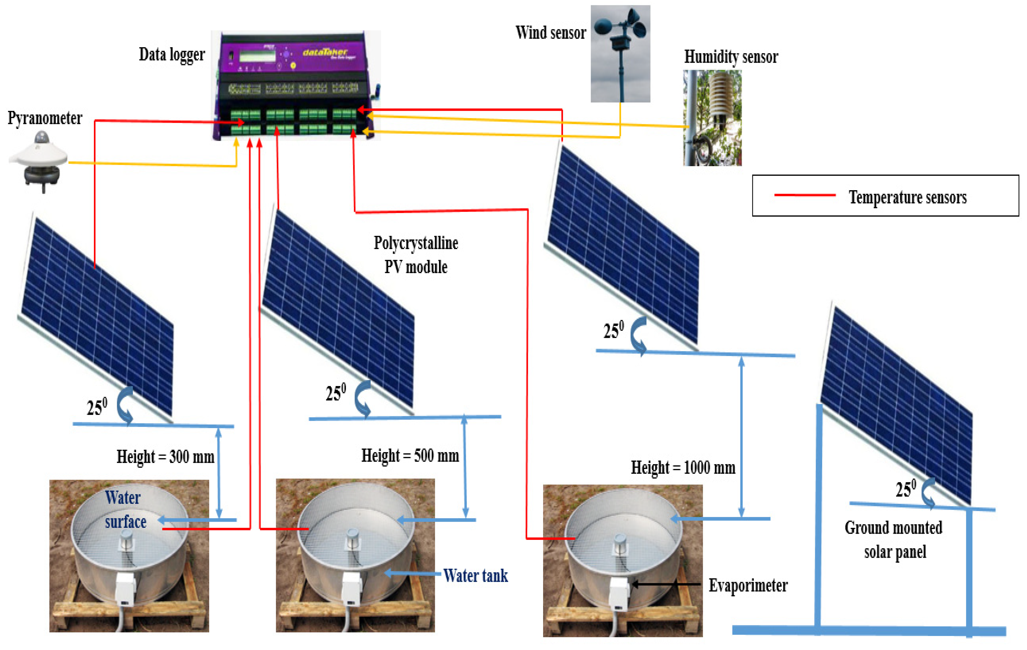
Figure 1. Outline of experimental setup at BITS Pilani, Rajasthan (India).
Energies 17 03489 g001
Figure 2. Experimental Setup in the Field: Floating PV and Ground mounted installations.
Energies 17 03489 g002
Figure 3. Predicted panel temperature for the typical day with maximum solar insolation in May 2021 (A) All eight models, Kamuyu et al. (2018) [33] models and recorded temperature (B) Four best performing models F1, F2, F3, F4, and recorded panel temperature.
Energies 17 03489 g003
Figure 4. Plots of predicted panel temperature by model F3 with respect to recorded panel temperature for summer months (May and June), winter (January and February), and monsoon season (July and August).
Energies 17 03489 g004
Figure 5. Power estimate for a typical day of maximum insolation in May 2021 (A) from recorded panel temperature data, estimates from the F1 to F8 model, and the models from Kamuyu et al. (2018) [33] (B) from recorded panel temperature data estimates from best-performing temperature models F1, F2, F3, F4 model.
Energies 17 03489 g005
Figure 6. Monthly energy generation of Ground-mounted and floating PV installation for (a) maximum and (b) minimum solar insolation day of each month from April 21–March 22.
Energies 17 03489 g006
Table 1. PV panel temperature prediction models by various authors.
AuthorYearEquationType of MountingParameters
Ross [36]1976 T m o d = T a + k G T Ground Mountedk—empirical constant
Rauschenbach [37]1980 T c = T a + G T G N O C T . T c N O C T T a N O C T . 1 η m τ α Ground MountedTcNOCT Cell nominal operating temperature,°C TaNOCT Ambient temperature according to SRE, set at 20 °C GNOCT Total irradiance according to SRE, set at 800 W/m², Tc Cell Temperature in °C. η m = η c τ α , η c —conversion efficiency of module.
Risser and Fuentes [13]1983 T m o d = 0.899 T a + 3.12 + 0.025 G T 1.30 V w Ground MountedTmod—module temperature in °C
Schott [4]1985 T m o d = T a 1 + 0.028 G T Ground MountedGT—Solar insolation in W/m2
Ross and Smokler [8]1986 T m o d = T a + 0.035 G T Ground MountedVw—wind velocity in m/s
Irodionov et al. [19]1989 T m o d = 0.7 + 0.0155 G T + T a Ground MountedTa—ambient temperature in °C
Lasnier and Ang [6]1990 T m o d = 30.006 + 0.0175 G T 150 + 1.14 T a 25 Ground MountedTmodK—module temperature in K
Markvart [38]2000 T m o d = 0.943 T a + 4.3 + 0.028 G T 1.528 V w Ground MountedTaK—ambient temperature in K
King et al. [39]2004 T m o d   = T a + G T e 3.47 0.0594 V w Ground Mounted
Mattei et al. [40]2006 T m o d = U T a + G T α τ η r e f β p o w e r η r e f T m o d , r e f U β p o w e r η r e f G T Ground MountedU—heat exchange coefficient of module
α —cell absorption coefficient
τ—glass transmittance
ηref—the module efficiency at reference temperature
T m o d , r e f —25 °C
β p o w e r —power variation coefficient
Faiman [24]2008 T m o d K = T a K + G T U 0 + U 1 . V w Ground Mounted
Skoplaki et al. [10]2008 T m o d K = T a K + 0.32 8.91 + 2 V w G T Ground Mounted
Muzathik [12]2014 T m o d = 0.943 T a + 0.35229 + 0.0195 G T 1.528 V w Ground Mounted
Coskun et al. [9]2016 T m o d = 1.4 T a + 0.01 G T 500 V w 0.8 Ground Mounted
Kamuyu et al. [33]2018Tm1 = 2.0458 + 0.9458Ta + 0.0215 GT − 1.2376Vw
Tm2 = 1.8081 + 0.9282Ta + 0.021GT − 1.2210Vw + 0.0246Tw
Water Mounted
Table 2. Variables and R2 values for the exponential model for ground-mount and floating PV.
Type of MountingR2VariablesModel Nomenclature
Ground-mounted0.737 G T , v, T a GM1
Water mounted0.955 G T , v, T a F1
Water mounted0.94 G T , v, T w F2
Table 3. Regression models for floating PV.
ModelR2VariablesModel Nomenclature
Linear Regression Degree 010.956 G T , v, T a F3
Linear Regression Degree 010.93 G T , v, R h , T w F4
Linear Regression Degree 010.96 G T , v, R h , T a , T w F5
Linear Regression Degree 020.96 G T , v, T a F6
Linear Regression Degree 020.944 G T , v, R h , T w F7
Linear Regression Degree 020.963 G T , v, T a , T w , R h F8
Table 4. Maximum and minimum RMSE for temperature predicted by models.
RMSEModels
F1F2F3F4F5F6F7F8
Maximum5.648.265.509.438.196.9522.3822.07
Minimum1.962.651.672.345.492.5411.3511.90
Bold is for the best performing model.
Table 5. RMSE of temperature prediction for different seasons.
RMSEModels
F1F2F3F4F5F6F7F8
Summer7.427.217.308.2710.818.9920.2120.07
Monsoon2.613.662.743.365.313.3113.5013.34
Winter3.114.193.073.955.283.7411.5813.04
Correlation coefficient
Summer0.900.890.900.900.870.890.880.87
Monsoon0.970.950.970.960.970.970.930.92
Winter0.980.950.970.960.970.970.950.93
R2
Summer0.810.790.810.810.750.790.770.75
Monsoon0.940.900.940.920.930.930.870.85
Winter0.950.910.950.910.940.950.900.87
Bold is for the best performance.
Table 6. Energy estimate of 24 days in a year (April 2021–March 2022) using maximum and minimum insolation days in each month and percentage error w.r.t recorded data.
Recorded DataModel F1Model F2Model F3Model F4Model F5Model F6Model F7Model F8
Energy Estimated (Wh)20,37220,29320,30320,36220,30919,63919,99918,43518,410
% above/below the Recorded data −0.53−0.49−0.20−0.46−3.74−1.98−9.64−9.76
Bold is for the best performance.
Table 7. Seasonal variations on energy estimate of 24 days in a year (April 2021–March 2022) using maximum and minimum insolation days in each month and percentage error with respect to recorded data.
SeasonEnergy Estimate with Recorded Panel Temperature DataEnergy Estimate with Modelled Panel Temperature Data
Model F1Model F2Model F3Model F4Model F5Model F6Model F7Model F8
SummerPower Estimated in Wh780977167723778277247474760469947000
% above or below the Recorded data −1.19−1.10−0.35−1.09−4.29−2.63−10.44−10.36
MonsoonPower Estimated in Wh531752965295526152845125523847854795
% above or below the Recorded data −0.39−0.41−1.05−0.62−3.61−1.49−10.00−9.82
WinterPower Estimated in Wh727672817285731973017040715766566615
% above or below the Recorded data 0.070.120.590.34−3.24−1.64−8.52−9.08
AnnualPower Estimated in Wh20,40220,29320,30320,36220,30919,63919,99918,43518,410
% above or below the Recorded data −0.53−0.49−0.20−0.46−3.74−1.98−9.64−9.76
Bold is for the best performance.
Table 8. Seasonal maximum, minimum, and average panel operating temperature of floating and. Ground-mounted panels.
SeasonSummerWinterMonsoon
Panel over Water Bodies (°C)Panel over Ground Mount (°C)Panel over Water Bodies (°C)Panel over Ground Mount (°C)Panel over Water Bodies (°C)Panel over Ground Mount (°C)
Maximum Temperature66.6870.8659.5763.7365.5570.87
Minimum Temperature14.0213.45−0.86−1.3724.2624.38
Average Temperature39.5046.7725.7129.0638.3339.77
Bold is to highlight the impact of FSPV.
Table 9. Energy output for maximum and minimum solar insolation day in a year. (April 2021–March 2022).
MonthEnergy Generated (Floating) Maximum Insolation Day (Wh)Energy Generated (Floating) Minimum Insolation Day (Wh)Energy Generated (GM) Maximum Insolation Day
(Wh)
Energy Generated (GM) Minimum Insolation Day (Wh)
Apr-211280.7555.51238.4541.0
May-211258.1188.71226.7188.3
Jun-211295.1747.21258.6758.2
Jul-211261.7462.51293.1458.6
Aug-211283.9361.61248.5355.8
Sep-211120.9504.21090.7491.8
Oct-211219.9292.11194.3288.6
Nov-21953.9634.6926.2622.4
Dec-21981.7203.1952.1201.7
Jan-221105.3213.11066.9211.5
Feb-221245.0427.61198.2422.9
Mar-221307.41038.01256.7946.3
Disclaimer/Publisher’s Note: The statements, opinions and data contained in all publications are solely those of the individual author(s) and contributor(s) and not of MDPI and/or the editor(s). MDPI and/or the editor(s) disclaim responsibility for any injury to people or property resulting from any ideas, methods, instructions or products referred to in the content.