Interval Type-2 Fuzzy Logic Control of Linear Stages in Feedback-Error-Learning Structure Using Laser Interferometer

Abstract

The output processer of interval type-2 fuzzy logic systems (IT2FLSs) is a complex operator which performs type-reduction plus defuzzification (TR+D) tasks. In this paper, a complexity-reduced yet high-performance TR+D for IT2FLSs based on Maclaurin series approximation is utilized within a feedback-error-learning (FEL) control structure for controlling linear move stages. IT2FLSs are widely used for control purposes, as they provide extra degrees of freedom to increase control accuracies. FEL benefits from a classical controller, which is responsible for providing overall system stability, as well as a guideline for the training mechanism for IT2FLSs. The Kalman filter approach is utilized to tune IT2FLS parameters in this FEL structure. The proposed control method is applied to a linear stage in real time. Using an identification process, a model of the real-time linear stage is developed. Simulation results indicate that the proposed FEL approach using the Kalman filter as an estimator is an effective approach that outperforms the gradient descent-based FEL method and the proportional derivative (PD) classical controller. Motivated by the performance of the proposed Kalman filter-based FEL approach, it is used to control a linear move stage in real time. The position feedback of the move stage is provided by a precision laser interferometer capable of performing measurements with an accuracy of less than $1\mathsf{\mu }\mathrm{m}$. Using this measurement system in a feedback loop with the proposed control algorithm, the overall steady state of the system is less than $20\mathsf{\mu }\mathrm{m}$. The results illustrate the high-precision control capability of the proposed controller in real-time.

1. Introduction

Advanced metrology equipment and methods are developing in response to the ever-increasing demand for precision object handling and manipulation within manufacturing environments using industrial robots [1,2]. The robotic applications within a manufacturing environment include additive manufacturing [3], precision assembly [4,5], and welding [6], to mention some of them. The positional accuracy of these robotic applications is affected by gearbox ratios, limited accuracy in joint angle encoders, geometrical uncertainties including robot link dimensions, assembly tolerances, structural deformation, and wear and tear of the industrial robot or robotic manipulator. To increase the positional accuracy of the robots, it is required to use advanced closed-loop control approaches [7,8,9,10,11] for position feedback through non-contact [12] or contact metrology equipment [13,14].

Among advanced control approaches, fuzzy logic control methods are of high interest due to the function approximation capability of these types of controllers. They have further applications in a wide range of applications, including wind power systems control [15] and image encryption [16]. Within the precision control field of study, advanced control approaches are emerging topics to improve the precision of manipulators, including the linear move stages for precision object handling and manipulation [17,18,19]. Modularized linear and rotational stage technology can be used for high-precision manipulation with micrometer- [20,21,22,23] and nanometer-scale accuracy [24,25]. They can be utilized within different applications, including but not limited to nano- and micro-positioning [26,27,28], and coordinate measurement machines [29]. Among advanced control approaches, IT2FLSs are widely known to be flexible control structures which benefit from the general function approximation capabilities of IT2FLSs. Furthermore, they are shown to be a robust type of controllers, capable of handling noise and uncertainties within the system [30,31].

The motor frequently used in a linear stage is a rotational one. To convert its rotational motion to a linear motion, a precision lead screw converter is commonly used. Multiple supportive bars with joints and fasteners may be used to provide extra support. However, using these support bars may result in friction forces in the structure [32]. Angular motor imperfection, lead screw converter imperfections, and the limited shaft encoder resolution may also result in increasing errors in the overall open-loop positioning of the motion system. Among all sources of uncertainty, friction forces acting on the lead screw and friction forces acting on the free moving bars are complicated to model using mathematical modelling techniques. In this paper, to handle the errors caused by these uncertainties, a closed-loop controller that utilizes interval type-2 fuzzy logic systems (IT2FLSs) with Maclaurin series approximate type-reduction and defuzzification (TR+D) in FEL structure is preferred. Highly accurate position feedback is provided using non-contact metrology equipment which operates based on the principles of interferometry. Accurate absolute industrial robot position can be provided using existing commercial non-contact metrology instruments. One of the frequently used non-contact metrology instruments is the laser interferometer. The laser interferometer used in this paper is a laser interferometer capable of performing position measurement in a straight line with a measurement accuracy of $\pm 0.5\mathrm{p}\mathrm{p}\mathrm{m}$.

IT2FLSs are a type of fuzzy logic systems [33,34] in which the membership functions and/or the consequent part parameters are interval values rather than crisp values [35,36]. The added degrees of freedom to the controller by having interval membership functions and interval consequent part parameters can be utilized to improve tracking performance. IT2FLS output calculations, including an output processing unit which performs the TR+D process, have been investigated in the literature. The first category of TR+D tasks includes the ones which do not include any approximation. The enhanced Karnik–Mendel approach [37], the enhanced opposite direction search algorithm [38], and the approach proposed in [39] that eliminates the requirement for sorting within the consequent part parameters can be named as three main approaches. The second category of TR+D tasks includes the approximate ones which benefit from lower complexity than accurate TR+D approaches. Some approaches in this category are Begian–Melek–Mendel [40], the Nie-Tan approach [41], and the Maclaurin series approximate solution [42]. Among the approximate approaches, the latter is the most accurate one [42] and is therefore the preferred method within this paper for IT2FLSs.

FEL is a control structure in which a classical controller works in parallel with an artificial intelligence structure, such as an IT2FLS. While the classical controller is responsible for controlling the closed-loop system, the parallel artificial intelligence structure improves the performance of the overall system. The classical controller in the loop provides guidelines for the intelligent structure. Gradient descent (GD) and the Kalman filter (KF) may be used to estimate the parameters of the parallel artificial intelligence structure, in this case, the IT2FLS. This approach has already been used to control load frequency systems [43], a selective compliance assembly robot arm [44], and an antilock braking system [45].

In this paper, the KF update rule is used to adapt the parameters of an IT2FLS in an FEL learning structure to control a linear stage. In an FEL structure, while a classical PD controller stabilizes the system in a closed loop, the IT2FLS improves the overall system performance. Motivated by the high performance of a KF in estimation tasks, this method is utilized to estimate the IT2FLS parameters. The results obtained from simulating this structure are compared with those of a case when the classical control approach works alone and a case when GD is used to train the IT2FLS. The simulation results demonstrate the superior performance of the FEL structure when a KF is used as its estimator to train an IT2FLS over other investigated approaches: the case when a classical PD controller is used and the case when an IT2FLS within an FEL is trained using GD. The main contribution of this paper is therefore to combine state-of-the-art metrology equipment, a laser interferometer, with advanced control methodology in an FEL control approach using an IT2FLS with a KF estimator to design a highly accurate linear positioning system to perform object manipulation across many application areas. To the best knowledge of the authors, feedback from laser interferometers has never been used within an FEL structure in a control structure before. Using the laser interferometer position feedback, it is possible to enhance the accuracy of the linear stage to less than a few micrometers in the workspace of a straight line. It is further to be noted that while GD uses a constant learning rate, the KF benefits from an adaptive covariance matrix which keeps a memory of all previous updates to the parameters of IT2FLSs and improves the overall performance of the controller. The proposed approach to control linear stages is then implemented on a real linear stage using the feedback provided by the laser interferometer. It is shown that using the laser interferometer position feedback, it is possible to enhance the accuracy of the linear stage to less than a few micrometers in the workspace of a straight line.

This paper is organized as follows: the methodology is given in Section 2. The experimental setup is given in Section 3. The mathematical model for the linear stage is explained in Section 4. The simulation results are presented in Section 5. The implementation results are given in Section 6, followed by concluding remarks in Section 7.

2. Methodology

2.1. Interval Type-2 Fuzzy Structures

IT2FLSs (see Figure 1) use interval type-2 fuzzy membership functions (IT2MFs) which have interval values for their grade of membership. There exist different IT2MFs: Gaussian IT2MFs with interval mean values and Gaussian IT2MFs with interval sigma values. In this paper, Gaussian IT2MFs with interval sigma values are utilized (see Figure 2). The shaded area in Figure 2 represents the footprint of uncertainty for the IT2MF. A rule in IT2FLSs is as follows:

$$\begin{array}{c}\mathit{j-th}rule:IF{x}_{1}is{\tilde{A}}_{j1}and{x}_{2}is{\tilde{A}}_{j2}\\ THEN{y}_j={\alpha }_{1j}{x}_1+{\alpha }_{2j}{x}_2+{\beta }_j,\left(j=1,\dots ,M\right),\end{array}$$

(1)

where $x_1$ and $x_2$ are the two inputs for the IT2FLS, $y$ is its output, and M is the total number of rules in the IT2FLS. Moreover, ${\tilde{A}}_{ji}$’s, (i = 1, 2) are interval type-2 fuzzy sets for $\mathit{jth}$ rule of the $\mathit{ith}$ input. The parameters ${\alpha }_{ij}$ and ${\beta }_j$ $(i=1,2,j=1,\dots ,M)$ are consequent part parameters.

$$\begin{array}{c}{F}_j={\alpha }_{1j}{x}_1+{\alpha }_{2j}{x}_2+{\beta }_j,\left(j=1,\dots ,M\right),\\ {\underset{\_}{w}}^j\left(x\right)={\underset{\_}{\mu }}_{{\tilde{F}}_1^j}\left(x_1\right)\ast {\underset{\_}{\mu }}_{{\tilde{F}}_2^j}\left(x_2\right),\left(j=1,\dots ,M\right),\\ {\overline{w}}^j\left(x\right)={\overline{\mu }}_{{\tilde{F}}_1^j}\left(x_1\right)\ast {\overline{\mu }}_{{\tilde{F}}_2^j}\left(x_2\right),\left(j=1,\dots ,M\right),\end{array}$$

(2)

where ${\underset{\_}{\mu }}_{{\tilde{F}}_k^j}\left(x_k\right),k=1,2$ and ${\overline{\mu }}_{{\tilde{F}}_k^j}\left(x_k\right),k=1,2$ form the IT2MFs.

To approximate the TR+D of an IT2FLS, Maclaurin series expansion is used as follows [42,46]:

$$y\in [y_l,y_r]$$

(3)

where $y_l$ and $y_r$ are the left-most and right-most values of output of IT2FLSs.

$$y_r\approx \frac{\sum _{j=1}^M({\overline{w}}^j+{\underset{\_}{w}}^j)F^j+\sum _{j=1}^M\left(sign\right({\overline{m}}^j\left)\mathsf{\Delta }{w}^j{F}^j\right)}{\sum _{j=1}^M({\overline{w}}^j+{\underset{\_}{w}}^j)+\sum _{j=1}^M\left(sign\right({\overline{m}}^j\left)\mathsf{\Delta }{w}^j\right)}$$

(4)

where the following applies:

$${\overline{m}}^j=F^j-\frac{\sum _{j=1}^M{\overline{w}}^j{F}^j}{\sum _{j=1}^M{\overline{w}}^j}$$

(5)

and $\mathsf{\Delta }{w}^j={\overline{w}}^j-{\underset{\_}{w}}^j$. Furthermore, $y_l$ is calculated as follows:

$$y_l\approx \frac{\sum _{j=1}^M({\overline{w}}^j+{\underset{\_}{w}}^j)F^j-\sum _{j=1}^M\left(sign\right({\underset{\_}{m}}^j\left)\mathsf{\Delta }{w}^j{F}_j\right)}{\sum _{j=1}^M({\overline{w}}^j+{\underset{\_}{w}}^j)-\sum _{j=1}^M\left(sign\right({\underset{\_}{m}}^j\left)\mathsf{\Delta }{w}^j\right)}$$

(6)

where the following applies:

$${\underset{\_}{m}}^j=F^j-\frac{\sum _{j=1}^M{\underset{\_}{w}}^j{F}^j}{\sum _{j=1}^M{\underset{\_}{w}}^j}$$

(7)

The parameter $Y\left(x\right)$, the output of the IT2FLS using the approximate TR+D of the IT2FLS, is then obtained as follows:

$$Y\left(x\right)=\frac{y_l+y_r}{2}$$

(8)

It is then possible to rewrite (5) as follows:

$$y_r=\sum _{j=1}^M{\nu }_R^j{F}_R^j$$

(9)

where the following applies:

$${\nu }_R^j=\frac{{\overline{w}}^j+{\underset{\_}{w}}^j+sign\left({\overline{m}}^j\right)\mathsf{\Delta }{w}^j}{\sum _{j=1}^M({\overline{w}}^j+{\underset{\_}{w}}^j)+\sum _{j=1}^M\left(sign\right({\overline{m}}^j\left)\mathsf{\Delta }{w}^j\right)}$$

(10)

It is further possible to rewrite (10) in a vector form as follows:

$$y_r={\varphi }_R\theta$$

(11)

where the following applies:

$${\varphi }_R=[{\overrightarrow{\nu }}_R^T,{\overrightarrow{\nu }}_R^T{x}_1,{\overrightarrow{\nu }}_R^T{x}_2{]}^T$$

(12)

and ${\overrightarrow{\nu }}_R$ is defined as follows:

$${\overrightarrow{\nu }}_R=[{\nu }_R^1,\dots ,{\nu }_R^M{]}^T.$$

(13)

Furthermore, $\overline{\theta }$ is defined as ${\theta }_{(n+1).M}^T=[{\beta }_1,\dots ,{\beta }_M,{\alpha }_{11},\dots ,{\alpha }_{1M},{\alpha }_{21},\dots ,{\alpha }_{2M}]$. Similarly, $y_l$ in (7) is rewritten in a vector form as follows:

$$y_l=\sum _{j=1}^M{\nu }_l^j{F}_l^j$$

(14)

where the following applies:

$${\nu }_l^j=\frac{({\overline{w}}^j+{\underset{\_}{w}}^j)-\left(sign\right({\underset{\_}{m}}^j\left)\mathsf{\Delta }{w}^j\right)}{\sum _{j=1}^M({\overline{w}}^j+{\underset{\_}{w}}^j)-\sum _{j=1}^M\left(sign\right({\underset{\_}{m}}^j\left)\mathsf{\Delta }{w}^j\right)}$$

(15)

Furthermore,

$$y_l={\varphi }_L\theta$$

(16)

where the following applies:

$${\varphi }_L=[{\overrightarrow{\nu }}_L^T,{\overrightarrow{\nu }}_L^T{x}_1,{\overrightarrow{\nu }}_L^T{x}_2{]}^T$$

(17)

and ${\overrightarrow{\nu }}_L$ is defined as follows:

$${\overrightarrow{\nu }}_L=[{\nu }_L^1,\dots ,{\nu }_L^M{]}^T$$

(18)

The pseudocode for IT2FLS output calculation is given in Table 1.

2.2. Gradient Descent Training Approach

The gradient descent training approach [47] is a frequently used training method in the literature and is based on Taylor expansion of a quadratic loss function. The parameter adaptation law to minimize a loss function is in the opposite direction of its gradient with respect to its parameters [47]. Using this approach, it is possible to find the optimal parameters of a cost function after several iterations. The optimization step size is determined by the learning rate of the GD optimization approach. While a learning rate that is too large may result in an unstable result, too small of a value for learning rate may result in trapping the optimization algorithm in a local minimum. Hence, considering $J$ as a function of $\theta$, the update rule for its parameters is obtained as follows [45]:

$${\theta }_{k+1}={\theta }_k-\gamma \frac{\partial J}{\partial {\theta }_k}.$$

(19)

where the learning rate parameter $\gamma$ is a positive constant.

Table 1. The pseudocode to find the output of an IT2FLS.

Calculating the Output of the IT2FLS
Find the IT2MF’s values, ${\underset{\_}{\mu }}_{{\tilde{F}}_k^j}\left(x_k\right),k=1,2$$\mathrm{and}{\overline{\mu }}_{{\tilde{F}}_k^j}\left(x_k\right),k=1,2,$ as follows:
${\underset{\_}{\mu }}_{{\tilde{F}}_k^j}\left(x_k\right)=exp\left(-{\left(\frac{x_k-m_k}{{\underset{\_}{\sigma }}_k}\right)}^2\right),k=1,2$	(20)
${\overline{\mu }}_{{\tilde{F}}_k^j}\left(x_k\right)=exp\left(-{\left(\frac{x_k-m_k}{{\overline{\sigma }}_k}\right)}^2\right),k=1,2$	(21)
$\mathrm{Calculate}{\overline{w}}^j$$\mathrm{and}{\underset{\_}{w}}^j$$\mathrm{and}j=1,\dots ,M$ as follows:
${\overline{w}}^j={\overline{\mu }}_{{\tilde{F}}_1^j}\left(x_1\right){\overline{\mu }}_{{\tilde{F}}_2^j}\left(x_2\right),j=1,\dots ,M$ ${\underset{\_}{w}}^j={\underset{\_}{\mu }}_{{\tilde{F}}_1^j}\left(x_1\right){\underset{\_}{\mu }}_{{\tilde{F}}_2^j}\left(x_2\right),j=1,\dots ,M$	(22)
$\mathrm{Calculate}{\overline{m}}^j$$\mathrm{and}{\underset{\_}{m}}^j$$\mathrm{as}\mathrm{in}\left(6\right)\mathrm{and}\left(8\right),\mathrm{where}{F}^j$ is as defined as in (2).
$\mathrm{Calculate}{y}_r$$\mathrm{and}{y}_l$ as in (5) and (7).
$\mathrm{Calculate}y$ as in (9).

Table 1. The pseudocode to find the output of an IT2FLS.

Calculating the Output of the IT2FLS
Find the IT2MF’s values, ${\underset{\_}{\mu }}_{{\tilde{F}}_k^j}\left(x_k\right),k=1,2$$\mathrm{and}{\overline{\mu }}_{{\tilde{F}}_k^j}\left(x_k\right),k=1,2,$ as follows:
${\underset{\_}{\mu }}_{{\tilde{F}}_k^j}\left(x_k\right)=exp\left(-{\left(\frac{x_k-m_k}{{\underset{\_}{\sigma }}_k}\right)}^2\right),k=1,2$	(20)
${\overline{\mu }}_{{\tilde{F}}_k^j}\left(x_k\right)=exp\left(-{\left(\frac{x_k-m_k}{{\overline{\sigma }}_k}\right)}^2\right),k=1,2$	(21)
$\mathrm{Calculate}{\overline{w}}^j$$\mathrm{and}{\underset{\_}{w}}^j$$\mathrm{and}j=1,\dots ,M$ as follows:
${\overline{w}}^j={\overline{\mu }}_{{\tilde{F}}_1^j}\left(x_1\right){\overline{\mu }}_{{\tilde{F}}_2^j}\left(x_2\right),j=1,\dots ,M$ ${\underset{\_}{w}}^j={\underset{\_}{\mu }}_{{\tilde{F}}_1^j}\left(x_1\right){\underset{\_}{\mu }}_{{\tilde{F}}_2^j}\left(x_2\right),j=1,\dots ,M$	(22)
$\mathrm{Calculate}{\overline{m}}^j$$\mathrm{and}{\underset{\_}{m}}^j$$\mathrm{as}\mathrm{in}\left(6\right)\mathrm{and}\left(8\right),\mathrm{where}{F}^j$ is as defined as in (2).
$\mathrm{Calculate}{y}_r$$\mathrm{and}{y}_l$ as in (5) and (7).
$\mathrm{Calculate}y$ as in (9).

2.3. Kalman Filter Training Method

The derivation of the Kalman filter update rule for an IT2FLS has been previously performed in the literature [45,48]. Let the output of an IT2FLS be written as $y=h\left(X,\theta \right),$ and $X\in R^n$ is the input vector for the IT2FLS, and the IT2FLS parameter vector is given by $\theta \in R^N$. It is required to update $\theta$ parameters during the training procedure. The estimation algorithm is formulated as a nonlinear discrete time system as follows:

$$\begin{array}{c}{\theta }_{k+1}={\theta }_k+{\omega }_k\\ y_k=h\left({\theta }_k\right)+{\nu }_k,\end{array}$$

(23)

where the index k for the parameters indicates their time index. $\mathrm{M}\mathrm{o}\mathrm{r}\mathrm{e}\mathrm{o}\mathrm{v}\mathrm{e}\mathrm{r},$ noise sequences ${\omega }_k$ and ${\nu }_k$ are zero-mean Gaussian and independent of each other. The statistics associated with KF parameters are as follows:

$$\begin{array}{c}E\left({\omega }_k\right)=0,E\left({\omega }_k{\omega }_l^T\right)=Q{\delta }_{kl}\\ E\left({\nu }_k\right)=0,E\left({\nu }_k{\nu }_l^T\right)=R{\delta }_{kl},\end{array}$$

(24)

where $E\left(.\right)$ is the expectation operator and ${\delta }_{kl}$ is the Kronecker delta. Hence, $E\left({\omega }_k{\omega }_l^T\right)=Q{\delta }_{kl}$ means that $\omega$ is white noise, and its correlations with all its time shifts are equal to zero, except when the time shift is equal to zero. Using the Taylor expansion of the function $h\left(.\right)$, and neglecting higher-order terms, the Kalman update rule for ${\theta }_k$ parameters is obtained as in [45].

$$\begin{array}{c}{\theta }_{k+1}={\theta }_k+K_k\left[y_k-h\left({\theta }_k\right)\right]\\ K_k=P_k{H}_k{\left(R+H_k^T{P}_k{H}_k\right)}^{-1}\\ P_{k+1}=P_k-K_k{H}_k^T{P}_k+Q,\end{array}$$

(25)

$K_k$ in the above equation is called the Kalman gain, $P_k$ is the covariance matrix, and $H_k$ is the first-order Taylor expansion of h(.) for the unknown parameters $\theta$. The covariance matrix is updated at every time instance, and it keeps track of all previous update rules for the KF. This feature makes the KF a stronger adaptation mechanism for IT2FLSs when compared to GD with a constant learning rate.

2.4. Feedback Error Learning

The FEL structure was introduced by Kawato and Gomi to design a stable neural network structure [49].

The overall control structure is demonstrated in Figure 3, and in this case, a PD controller, is responsible for controlling the overall system and providing guidelines to tune the parameters of the IT2FLS. Therefore, the FEL structure used in this paper is a hybrid use of PD controllers and IT2FLSs in a single control loop. The PD control coefficients are $K_p\mathrm{a}\mathrm{n}\mathrm{d}{K}_d$ for the proportionate and differentiated terms, respectively.

A PD control signal is used for the training purposes of the IT2FLS using GD and KF adaptation laws, such that the PD controller output becomes equal to zero. As soon as the PD controller output is equal to zero, the IT2FLS takes over control and becomes responsible for controlling the system. However, changes in the reference signal may excite the classical controller and result in an output value that is different from zero. As soon as the output of the classical controller becomes different from zero, the training mechanism for the IT2FLS is triggered, and after a few control samples, the output of the IT2FLS becomes zero again, making the IT2FLS the dominant controller in the loop. Because of the nonlinear nature of the IT2FLS, it is expected that it captures the nonlinearities quickly and improves the overall performance of the closed-loop system.

3. Experimental Setup

The overall system setup includes a move stage which provides linear motion and a laser interferometer which is responsible for providing position feedback for the system (see Figure 4). These components are explained in this section.

3.1. Laser Interferometer

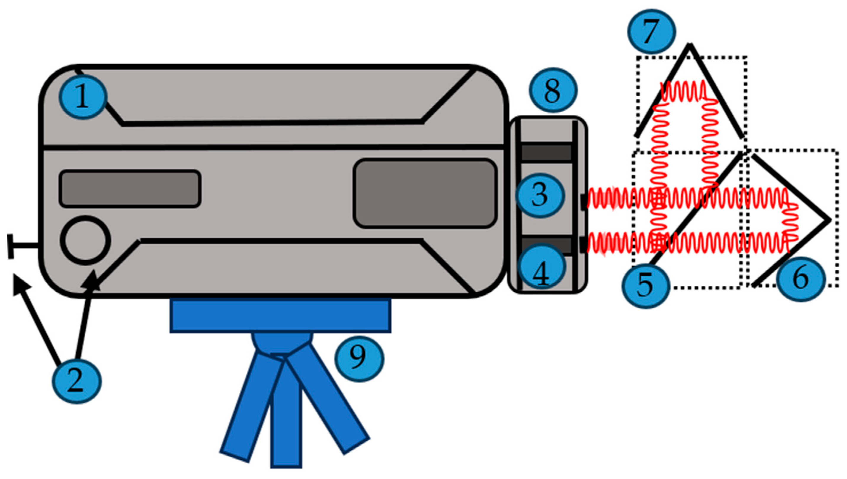
Laser interferometers are highly accurate laser measurement devices based on the principle of interference of light. A laser interferometer system includes a laser source/detector, a beam splitter, a static retroreflector, and a moving retroreflector (see Figure 5). Interference occurs between two laser beams: the outward beam and its return beam. While in the case of two in-phase laser beams, a bright fringe is produced in the detector unit, in the case when the two beams are 180° out of phase, a completely dark fringe is detected in the detector unit. The interference in the case of a Renishaw XL-80 occurs between a signal with a known travel distance and one with a fixed travel distance to the target retroreflector. The reference retroreflector is within a fixed distance of the detector unit within the Renishaw XL-80 (see Figure 5 and Figure 6). Renishaw XL-80 is manufactured by Renishaw company in Gloucestershire, UK. The components of the laser interferometer are summarized in

Table 2. Different components of laser interferometers.

1	Laser source and detector	6	Moving retroreflector
2	Adjustment screws for pitch and yaw of emitter/detector	7	Fixed retroreflector
3	Laser emitter	8	Rotating head
4	Laser detection	9	6 DoF adjustable bases
5	Beam splitter

. Because environmental conditions highly affect the measurements [50], an environmental weather station as part of the Renishaw XC-80 environmental compensation unit is used to work with the Renishaw XL-80 laser interferometer to compensate for these environmental changes (see Figure 6). The effects of environmental conditions, such as air pressure, air temperature, and air humidity, on the interferometer are compensated using the Renishaw XC-80 environmental compensation unit manufactured by Renishaw [50]. The Renishaw XL-80 is capable of detecting the direction of movement and can measure directional distance. This feature gives the flexibility to perform bidirectional movement measurements.

3.2. Linear Stage

A linear stage which is manufactured by Zaber^® in Vancouver, BC, Canada is used in this experiment. Linear stages are intended for but are not limited to medical purposes, marine applications [51], the aviation industry, and 3D printing [52,53]. One can handle a 250 N load using its two-phase stepper motor with a motor current rating of 600 mA/phase. It further uses a precision lead screw to convert stepper motor rotational movement to linear on the load side.

Although the communication protocol to provide connectivity is either Zaber ASCII or Zaber binary, under Python API, Zaber ASCII protocol is used. An RS232/USB converter eases the connectivity to readily available USB ports on the PC, and the maximum permeable connection baud rate for the move stages used in this study is 115,200 bps. The home position for the linear stage is provided by a magnetic hall sensor. This product is controllable from a PC using Python 3 using the manufacturer-provided Python library (https://www.zaber.com/software, accessed on 20 May 2024).

4. System Modelling Procedure

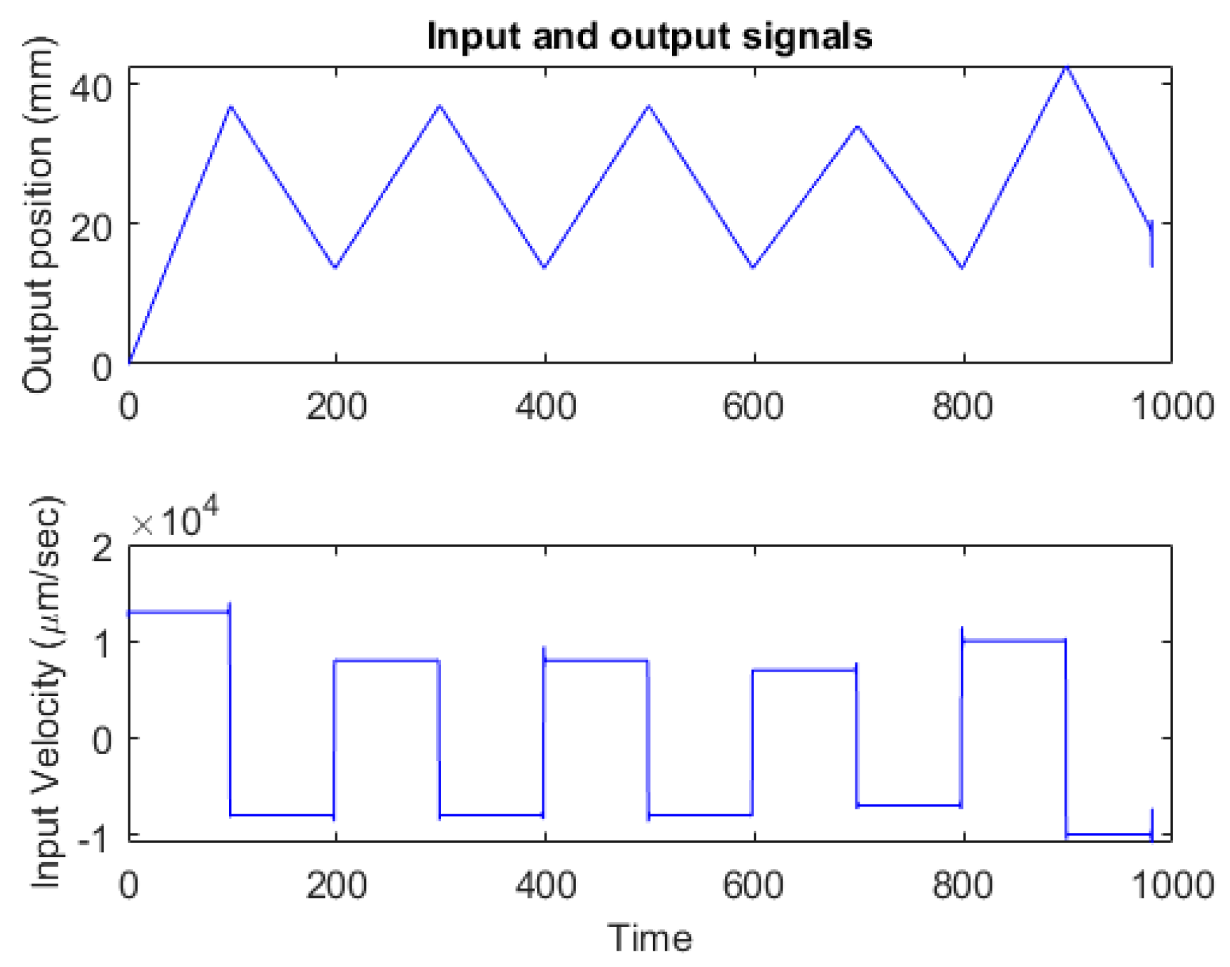
To model the move stage, a variable-amplitude input velocity is applied to the move stage. Figure 7 demonstrates different input signals applied to the linear stage. The output values are recorded using the laser interferometer and are illustrated in Figure 7. The spectrum analysis of the input and output data is given in Figure 8.

Using the system identification toolbox of MATLAB 2023, three different systems are generated for this dataset. The first system is considered to have just a single pole in the system. The second system is designed to have two poles in the system, and the last system is assumed to have two poles and a single zero in its structure. The three identified dynamic models are given as follows:

$$\begin{array}{c}{\mathrm{S}\mathrm{y}\mathrm{s}}_1=\frac{2.904\times {10}^{-5}}{\mathrm{s}+1.024\times {10}^{-17}}\\ {\mathrm{S}\mathrm{y}\mathrm{s}}_2=\frac{4.961\times {10}^{-5}}{{\mathrm{s}}^2+1.706\mathrm{s}+1.643\times {10}^{-6}}\\ {\mathrm{S}\mathrm{y}\mathrm{s}}_3=\frac{-1.589\times {10}^{-5}\mathrm{s}+7.661\times {10}^{-5}}{{\mathrm{s}}^2+2.635\mathrm{s}+2.477\times {10}^{-6}}\end{array}$$

(26)

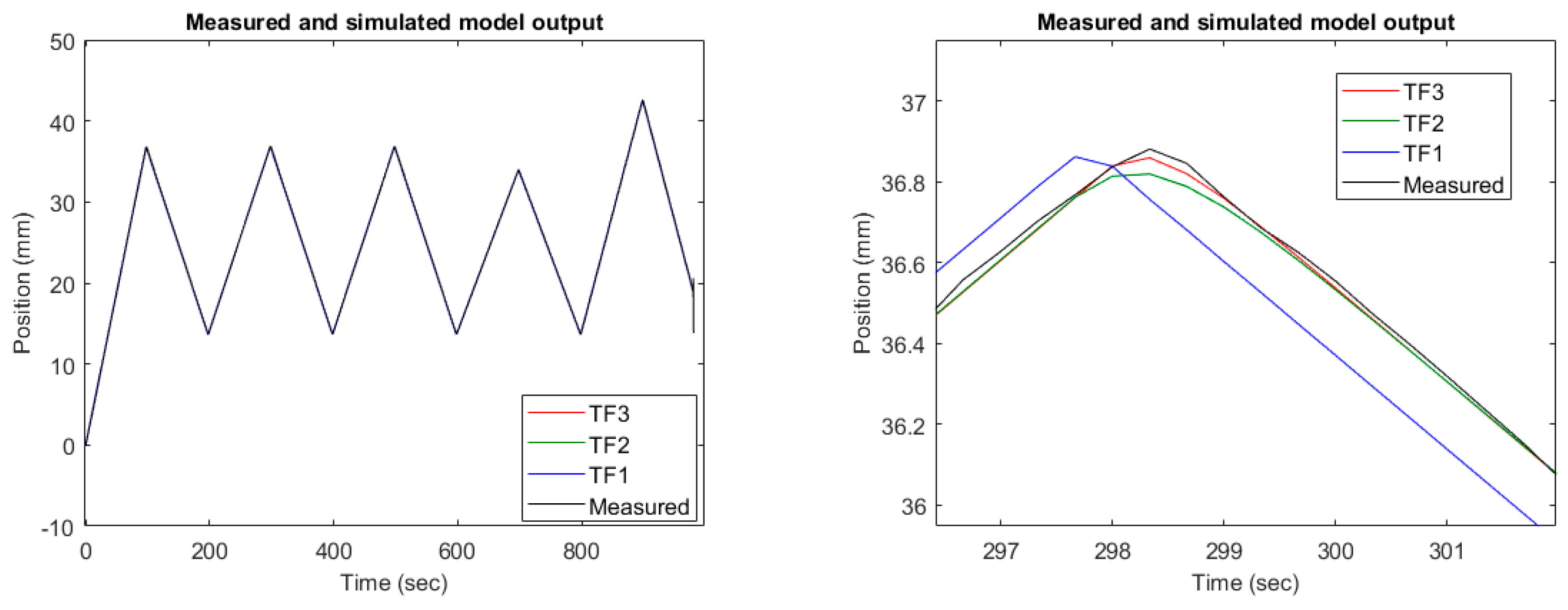
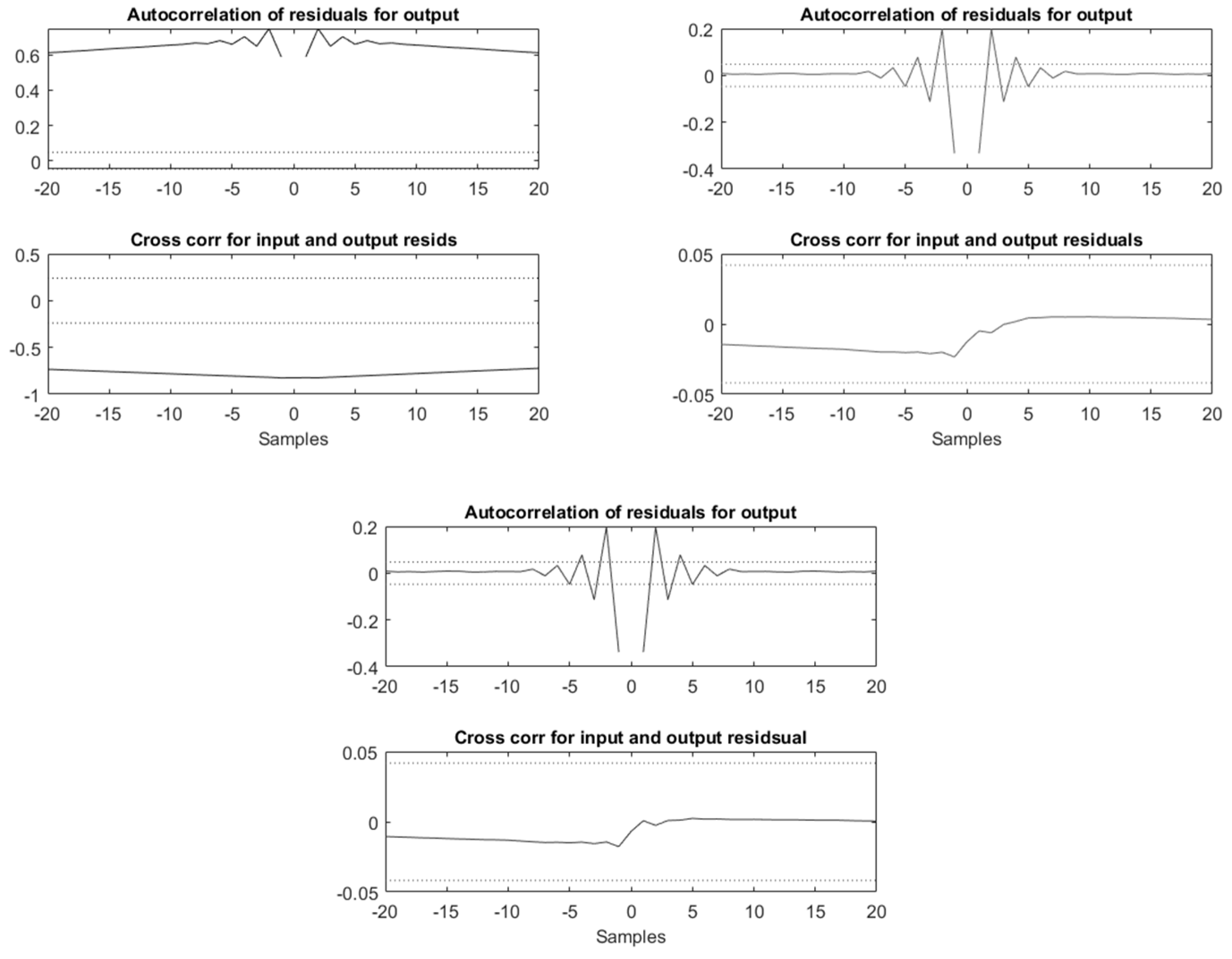
Figure 9 illustrates the time response of the three systems, and the correlations between the residual output and the input values for the three systems are given in Figure 10. While the mean squared error for identification in time domain for ${\mathrm{S}\mathrm{y}\mathrm{s}}_1$ is equal to 0.03274, it is 0.01027 for ${\mathrm{S}\mathrm{y}\mathrm{s}}_2$ and 0.01025 for ${\mathrm{S}\mathrm{y}\mathrm{s}}_3$. Therefore, according to Figure 10 and the given numerical values, the transfer functions ${\mathrm{S}\mathrm{y}\mathrm{s}}_2$ and ${\mathrm{S}\mathrm{y}\mathrm{s}}_3$ demonstrate superior transition response when they are compared to the measured values. However, between transfer functions ${\mathrm{S}\mathrm{y}\mathrm{s}}_2$ and ${\mathrm{S}\mathrm{y}\mathrm{s}}_3$, because of the lower degree of complexity for ${\mathrm{S}\mathrm{y}\mathrm{s}}_2$, this system is chosen as the preferred dynamic model for the linear stage.

5. Simulation Results

The linear stage is controlled using the proposed control structure, as demonstrated in Figure 3. This control structure benefits from IT2FLSs and the KF estimation method. The simulations are performed within a Simulink environment. Three IT2MFs are taken for the two input signals of $e$ and $\dot{e}$ (see Figure 11). The sample time taken to update the parameters of the IT2FLS is taken as equal to 324 ms. The covariance matrix, Q matrix, and R matrix for the KF are taken as follows:

$$R=2\times {10}^{-3},Q={10}^{-5}{I}_{18\times 18}$$

(27)

where $I_{18\times 18}$ is an $18\times 18$ identity matrix. For comparison purposes, the learning rate parameter value chosen for the GD algorithm is equal to $0.05$. We use ODE23s as the ordinary differential equation solver for a Simulink environment. This solver is a very robust and accurate ordinary differential equation solver that is the preferred one in this paper. The reference signals chosen for the system are two different step reference signals and a mixture of a ramp and a step signal. These reference signals are presented mathematically as follows:

$$r(t)=\left\{\begin{array}{cc}\begin{array}{c}2.5\times {10}^{-5}t\\ 0.01\\ 0.02\end{array}& \begin{array}{c}t\le 400\\ 400\le t<800\\ 800\le t<1200\end{array}\\ \begin{array}{c}\begin{array}{c}0.03\\ 0.02-\frac{1\times {10}^{-4}(\mathrm{t}-2000)}{3}\end{array}\\ \begin{array}{c}0\\ 0.01\end{array}\end{array}& \begin{array}{c}\begin{array}{c}1200\le t<2000\\ 2000\le t<2600\end{array}\\ \begin{array}{c}2600\le t<3200\\ 3200\le t\end{array}\end{array}\end{array}\right.$$

(28)

The assumed unit for the reference signal $r\left(t\right)$ is meters. The linear stage has a limitation of movement of 5 cm; therefore, the reference signal is designed such that it does not include any values out of this range. The dynamic system model obtained in the previous section is used to study the tracking performance of the proposed FEL controller. Using the reference signals, as in (28), and the control loop, as presented in Figure 3, simulations are performed. The PD parameter values are considered as follows:

$$K_p=1000,K_d=500$$

(29)

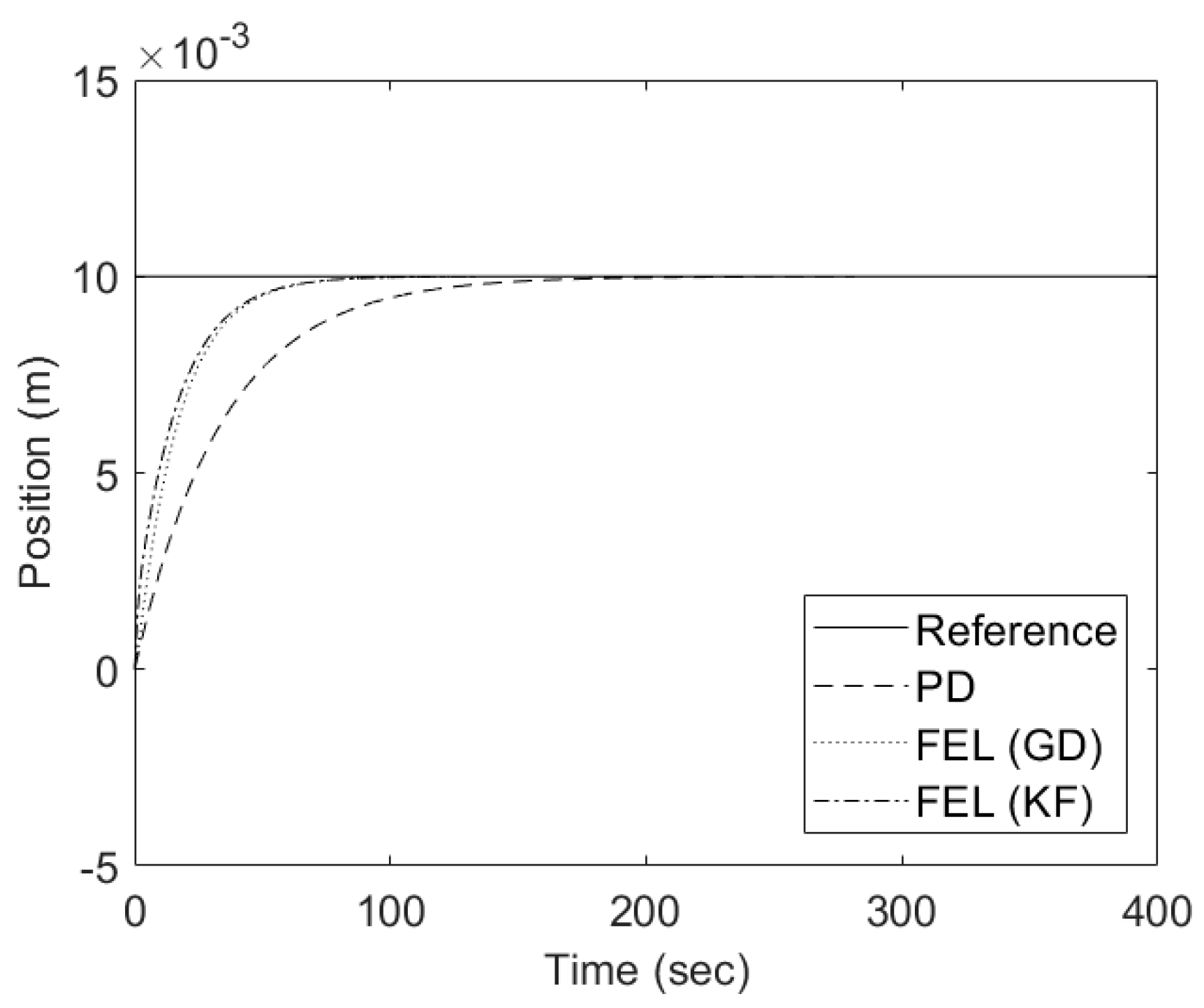
Figure 12 demonstrates the closed-loop step response for the system. As can be seen from the figure, when the proposed FEL control algorithm which benefits from a KF is used in the loop, the response converges to its reference signal more quickly. The integral of the squared error for the closed-loop system is presented in

Table 3. Integrals of squared errors for torque controllers.

Controller	$\mathbf{Step}\mathbf{Response}({\mathbf{m}}^2\mathbf{s}$)	$\mathbf{Mixed}\mathbf{Step}\mathbf{and}\mathbf{Ramp}\mathbf{Reference}({\mathbf{m}}^2\mathbf{s}$)	$\mathbf{Pulse}\mathbf{Response}({\mathbf{m}}^2\mathbf{s}$)
PD working alone	$1.72\times {10}^{-3}$	$8.30\times {10}^{-3}$	$2.24\times {10}^{-2}$
FEL GD	$8.86\times {10}^{-4}$	$3.94\times {10}^{-3}$	$1.16\times {10}^{-2}$
FEL KF	$66.9\times {10}^{-4}$	$3.68\times {10}^{-3}$	$1.02\times {10}^{-2}$

. As can be seen from the values presented in the table, in the case when the proposed FEL controller which benefits from a KF is used in the loop, the integral of the squared error is less than when GD is used for IT2FLS parameter estimation purposes. Moreover, the integral of the squared error is reduced considerably in the case when an FEL structure with KF estimation is used as compared to that in which the case PD controller is used in the feedback loop.

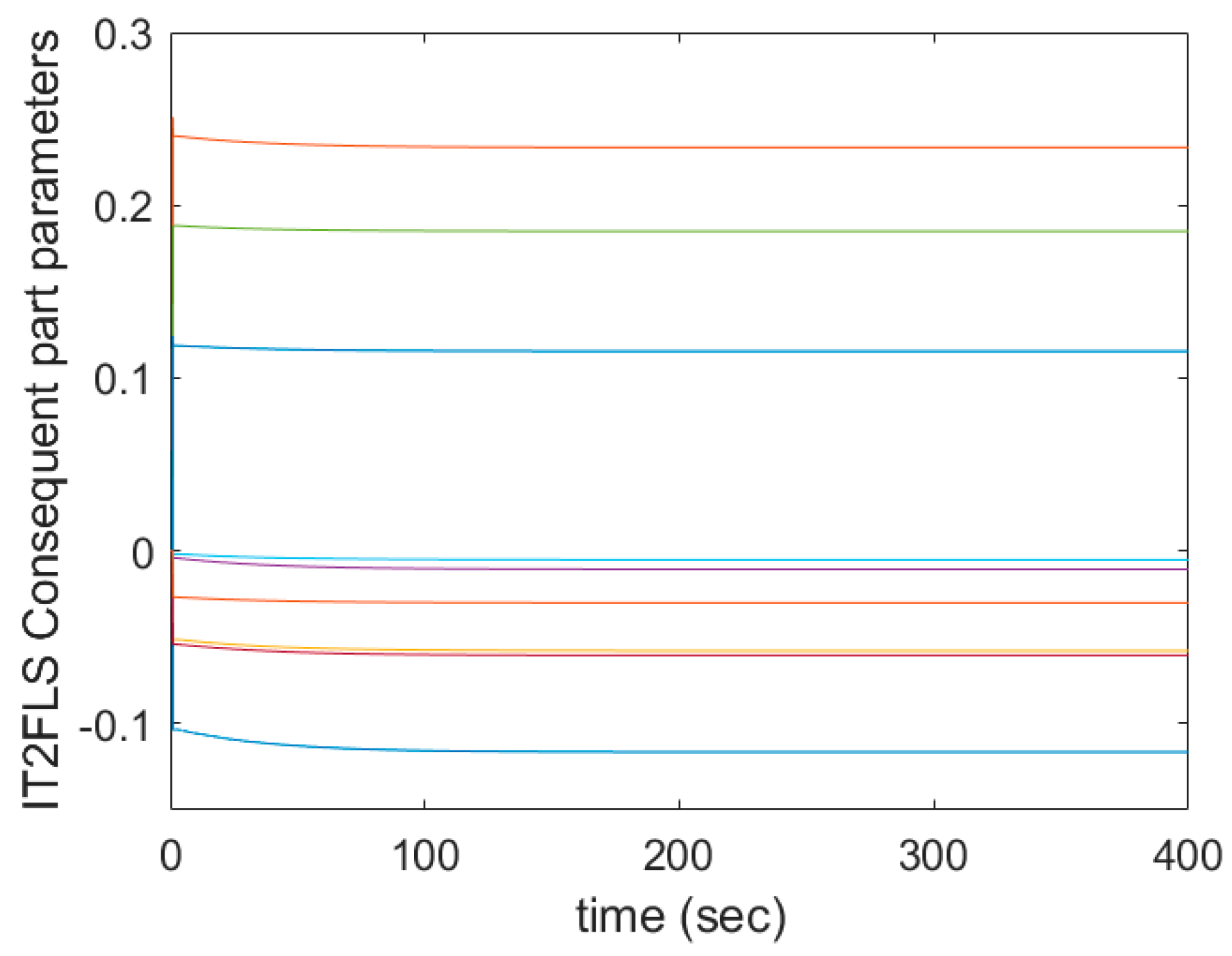
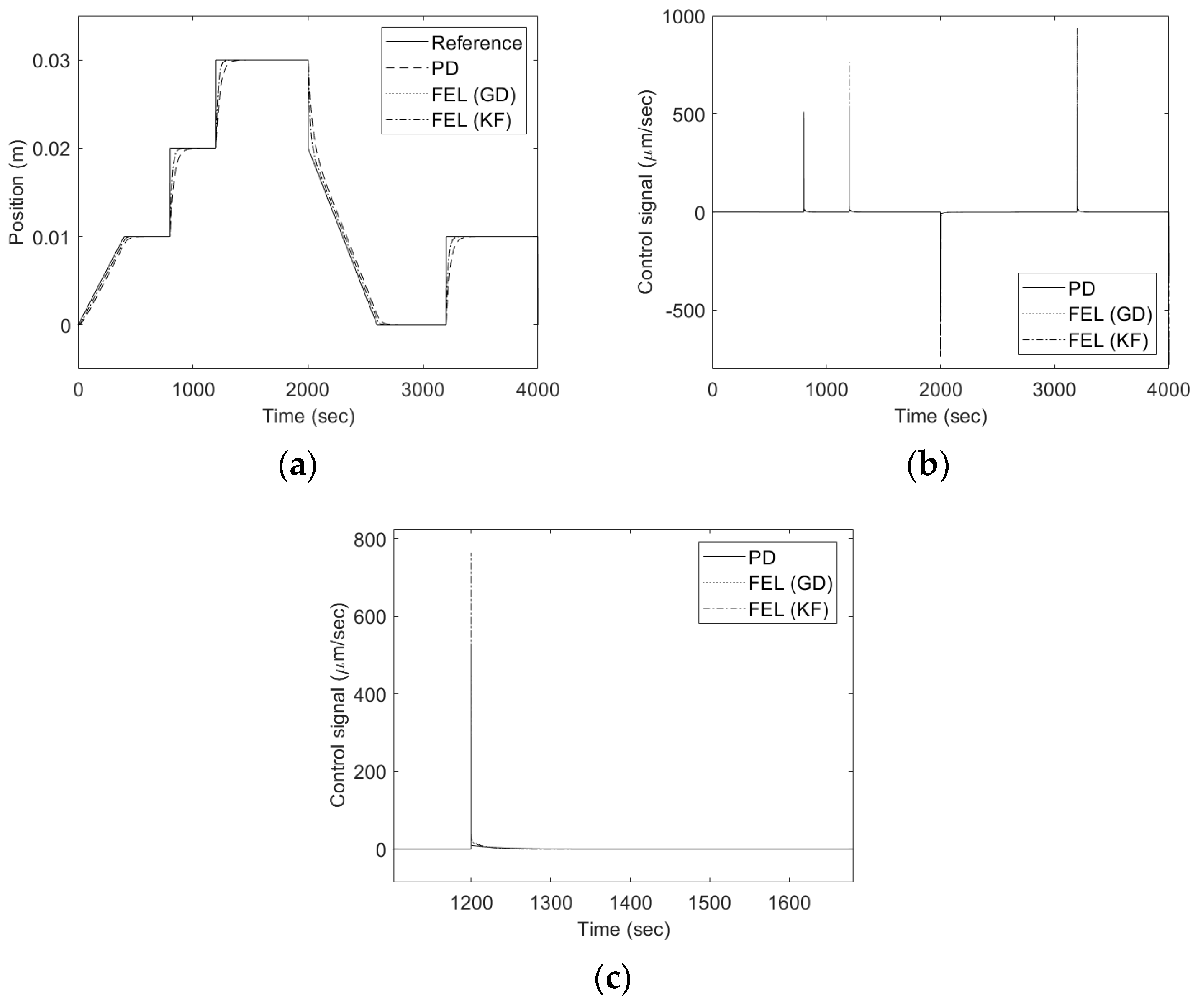
The consequent parameters of the IT2FLS are initialized as zero. The behavior of the IT2FLS parameters during adaptation when the reference signal is a step signal is depicted in Figure 13. This figure shows that the IT2FLS consequent part parameters converge to a value during adaptation, and no parameter drift is observed during their tunning phase. The response of the system when the reference signal is as in (28) is illustrated in Figure 14. As can be seen from the figure, the reference signal, which is a combinations of step changes and ramp signals, is tracked with high performance in this figure when an FEL structure with KF adaptation law is used. Comparison between the responses of the integrals of squared error for the three controllers are provided in Table 3. The results illustrate the superiority of the proposed FEL controller with KF adaptation law over the two other control approaches.

The response of the adaptive control scheme in the presence of multiple pulse reference signals is illustrated in Figure 15. The results demonstrate that the adaptive controller is stable in the presence of a pulse reference signal. Furthermore, the integrals of squared error provided in Table 3 illustrate that this index is 55.4% less for the FEL structure when it uses a KF as its estimator as compared to the PD control approach when it works alone.

6. Experimental Results

The control structure illustrated in Figure 3 is implemented on a single-axis real-time linear stage. The feedback is provided by a laser interferometer capable of performing measurements with an accuracy of up to $\pm 0.5\mathrm{p}\mathrm{p}\mathrm{m}$ and a resolution of up to 1 nm. Considering the available control commands for the Zaber move stage under Python API, the speed controller is implemented on the real-time linear stage. The control signal is updated every 324 ms. The main reason for such a slow sample time is the time delay caused by the laser interferometer. Motivated by the fact that the IT2FLS in FEL with a KF update rule outperforms the other studied control structures, such as a PD controller working alone and an IT2FLS in FEL with a GD update rule (see Section 2.4), this structure is the preferred algorithm in the implementation part. The initial values considered for IT2FLS are considered to be equal to zero, and the values are updated during the adaptation period. The overall experiment structure is as previously demonstrated in Figure 4. The laser interferometer in this setup is configured in line with the linear stage workspace line for precise measurements. Using the feedback provided by the laser interferometer, the entire feedback loop is implemented within Python 3 software. Multiple reference inputs in the form of step signals with different reference values are given. The closed-loop response of the controller and the control signal are depicted in Figure 16a. The steady-state errors (SSEs) for the system are 24 µm, 10 µm, and 6 µm for step reference signals of 10 mm, 15 mm, and 20 mm, respectively. The speed control signals are also shown in Figure 16b.

7. Conclusions

In this paper, a linear stage is controlled using an IT2FLS which benefits from a Maclaurin series approximate TR+D in an FEL structure. The KF is a powerful estimator which benefits from a covariance matrix and is used to train an IT2FLS in this paper. As compared to the GD algorithm, the covariance matrix in a KF algorithm provides an optimal update gain matrix for IT2FLS consequent part parameters which includes all previous regression values. The proposed FEL structure which benefits from the KF estimation technique is compared with an FEL structure with a GD structure and a classical PD controller when acting alone. Using simulation studies, it is observed that the proposed controller can control the 2D linear stage in the case of a step reference signal and a ramp reference signal with higher performance than the other two control approaches of a PD controller and an FEL with a GD estimation algorithm. When the KF is used in the FEL structure to tune the IT2FLS parameters, it outperforms the case in which GD is used. Moreover, it is observed that the integral of squared error in the case of the proposed controller is reduced considerably compared to the PD controller. Motivated by the results obtained within the simulations, the proposed control approach is implemented in closed loops on a real system, and the proposed control can control the linear stage system with steady-state errors in the order of a few micrometers.

In future work, the applications of the proposed FEL structure will be considered in the precision control of robotic manipulators for performing object handling and object manipulation by considering the stiffness and damping caused by the object.

References

1. Hu, J.; Li, C.; Chen, Z.; Yao, B. Precision motion control of a 6-DoFs industrial robot with accurate payload estimation. IEEE/ASME Trans. Mechatron. 2020, 25, 1821–1829. [Google Scholar] [CrossRef]
2. Nguyen, V.; Cvitanic, T.; Baxter, M.; Ahlin, K.; Johnson, J.; Freeman, P.; Balakirsky, S.; Brown, A.; Melkote, S. Precision robotic milling of fiberglass shims in aircraft wing assembly using laser tracker feedback. SAE Int. J. Aerosp. 2022, 15, 87–97. [Google Scholar] [CrossRef]
3. Yuan, L.; Ding, D.; Pan, Z.; Yu, Z.; Wu, B.; van Duin, S.; Li, H.; Li, W. Application of multidirectional robotic wire arc additive manufacturing process for the fabrication of complex metallic parts. IEEE Trans. Ind. Inform. 2019, 16, 454–464. [Google Scholar] [CrossRef]
4. Xiao, J.; Dou, S.; Zhao, W.; Liu, H. Sensorless human-robot collaborative assembly considering load and friction compensation. IEEE Robot. Autom. Lett. 2021, 6, 5945–5952. [Google Scholar] [CrossRef]
5. Fan, Y.; Luo, J.; Tomizuka, M. A learning framework for high precision industrial assembly. In Proceedings of the 2019 International Conference on Robotics and Automation (ICRA), Montreal, QC, Canada, 20–24 May 2019; pp. 811–817. [Google Scholar]
6. Rout, A.; Deepak, B.; Biswal, B. Advances in weld seam tracking techniques for robotic welding: A review. Robot. Comput. Integr. Manuf. 2019, 56, 12–37. [Google Scholar] [CrossRef]
7. Ghafarian, M.; Shirinzadeh, B.; Al-Jodah, A.; Das, T.K. Adaptive fuzzy sliding mode control for high-precision motion tracking of a multi-DOF micro/nano manipulator. IEEE Robot. Autom. Lett. 2020, 5, 4313–4320. [Google Scholar] [CrossRef]
8. García-Chávez, R.E.; Silva-Ortigoza, R.; Hernández-guzmáN, V.M.; Marciano-Melchor, M.; Orta-Quintana, Á.A.; García-Sánchez, J.R.; Taud, H. A Robust Sliding Mode and PI-Based Tracking Control for the MIMO “DC/DC Buck Converter–Inverter–DC Motor” System. IEEE Access 2023, 11, 119396–119408. [Google Scholar] [CrossRef]
9. de Jesús Rubio, J.; Orozco, E.; Cordova, D.A.; Hernandez, M.A.; Rosas, F.J.; Pacheco, J. Observer-based differential evolution constrained control for safe reference tracking in robots. Neural Netw. 2024, 175, 106273. [Google Scholar] [CrossRef]
10. de Jesús Rubio, J.; Hernandez, M.A.; Rosas, F.J.; Orozco, E.; Balcazar, R.; Pacheco, J. Genetic high-gain controller to improve the position perturbation attenuation and compact high-gain controller to improve the velocity perturbation attenuation in inverted pendulums. Neural Netw. 2024, 170, 32–45. [Google Scholar] [CrossRef]
11. de Jesús Rubio, J.; Hernandez, M.A.; Orozco, E.; Cordova, D.A.; Zacarias, A.; Pacheco, J. Observer-based model-free controller for the perturbations estimation and attenuation in robotic plants. Robot. Auton. Syst. 2024, 177, 104713. [Google Scholar] [CrossRef]
12. Zhang, J.; Lou, Z.; Fan, K.-C. Accuracy improvement of a 3D passive laser tracker for the calibration of industrial robots. Robot. Comput. Integr. Manuf. 2023, 81, 102487. [Google Scholar] [CrossRef]
13. Wan, Z.; Zhou, C.; Lin, Z.; Yan, H.; Tang, W.; Wang, Z.; Wu, J. An Improved Design of the MultiCal On-Site Calibration Device for Industrial Robots. Sensors 2023, 23, 5717. [Google Scholar] [CrossRef] [PubMed]
14. Wan, Z.; Zhou, C.; Zhang, H.; Wu, J. Development of an onsite calibration device for robot manipulators. Front. Inf. Technol. Electron. Eng. 2023, 24, 217–230. [Google Scholar] [CrossRef]
15. Yan, S.; Gu, Z.; Park, J.H.; Xie, X. Sampled memory-event-triggered fuzzy load frequency control for wind power systems subject to outliers and transmission delays. IEEE Trans. Cybern. 2022, 53, 4043–4053. [Google Scholar] [CrossRef] [PubMed]
16. Yan, S.; Gu, Z.; Park, J.H.; Xie, X. Synchronization of delayed fuzzy neural networks with probabilistic communication delay and its application to image encryption. IEEE Trans. Fuzzy Syst. 2022, 31, 930–940. [Google Scholar] [CrossRef]
17. Choi, J.; Baek, J.; Lee, W.; Lee, Y.S.; Han, S. Adaptive model-free control with nonsingular terminal sliding-mode for application to robot manipulators. IEEE Access 2020, 8, 169897–169907. [Google Scholar] [CrossRef]
18. Alhama Blanco, P.J.; Abu-Dakka, F.J.; Abderrahim, M. Practical use of robot manipulators as intelligent manufacturing systems. Sensors 2018, 18, 2877. [Google Scholar] [CrossRef] [PubMed]
19. Ning, Y.; Li, T.; Du, W.; Yao, C.; Zhang, Y.; Shao, J. Inverse kinematics and planning/control co-design method of redundant manipulator for precision operation: Design and experiments. Robot. Comput. Integr. Manuf. 2023, 80, 102457. [Google Scholar] [CrossRef]
20. Zhang, F.; Huang, Q.; Ye, Y.; Cheng, B.; Zhang, Z.; Cheng, R.; Zhang, L.; Li, H. Development of submicron precision three-dimensional low cross-interference air-floating motion stage. Rev. Sci. Instrum. 2023, 94, 065013. [Google Scholar] [CrossRef]
21. Chang, Q.; Liu, Y.; Deng, J.; Zhang, S.; Chen, W. Design of a precise linear-rotary positioning stage for optical focusing based on the stick-slip mechanism. Mech. Syst. Signal Process. 2022, 165, 108398. [Google Scholar] [CrossRef]
22. Al-Jodah, A.; Shirinzadeh, B.; Ghafarian, M.; Das, T.K.; Tian, Y.; Zhang, D. A fuzzy disturbance observer based control approach for a novel 1-DOF micropositioning mechanism. Mechatronics 2020, 65, 102317. [Google Scholar] [CrossRef]
23. Go, G.; Kwak, D.; Piao, L.; Choi, H.; Jeong, S.; Lee, C.; Park, B.J.; Ko, S.Y.; Park, J.-o.; Park, S. Manipulation of micro-particles using a magnetically actuated microrobot. Mechatronics 2013, 23, 1037–1043. [Google Scholar] [CrossRef]
24. Yang, P.; Takamura, T.; Takahashi, S.; Takamasu, K.; Sato, O.; Osawa, S.; Takatsuji, T. Development of high-precision micro-coordinate measuring machine: Multi-probe measurement system for measuring yaw and straightness motion error of XY linear stage. Precis. Eng. 2011, 35, 424–430. [Google Scholar] [CrossRef]
25. Manske, E.; Fröhlich, T.; Füßl, R.; Ortlepp, I.; Mastylo, R.; Blumröder, U.; Dontsov, D.; Kühnel, M.; Köchert, P. Progress of nanopositioning and nanomeasuring machines for cross-scale measurement with sub-nanometre precision. Meas. Sci. Technol. 2020, 31, 085005. [Google Scholar] [CrossRef]
26. Jeong, Y.; Dong, J.; Ferreira, P. Self-calibration of dual-actuated single-axis nanopositioners. Meas. Sci. Technol. 2008, 19, 045203. [Google Scholar] [CrossRef]
27. Korpelainen, V.; Lassila, A. Calibration of a commercial AFM: Traceability for a coordinate system. Meas. Sci. Technol. 2007, 18, 395. [Google Scholar] [CrossRef]
28. Xia, F.; Quigley, J.; Zhang, X.; Yang, C.; Wang, Y.; Youcef-Toumi, K. A modular low-cost atomic force microscope for precision mechatronics education. Mechatronics 2021, 76, 102550. [Google Scholar] [CrossRef]
29. Dang, Q.; Yoo, S.; Kim, S.-W. Complete 3-D self-calibration of coordinate measuring machines. CIRP Ann. 2006, 55, 527–530. [Google Scholar] [CrossRef]
30. Ochoa, P.; Castillo, O.; Melin, P.; Soria, J. Differential evolution with shadowed and general type-2 fuzzy systems for dynamic parameter adaptation in optimal design of fuzzy controllers. Axioms 2021, 10, 194. [Google Scholar] [CrossRef]
31. Kavikumar, R.; Sakthivel, R.; Kwon, O.M.; Kaviarasan, B. Robust model reference tracking control for interval type-2 fuzzy stochastic systems. IET Control Theory Appl. 2020, 14, 1123–1134. [Google Scholar] [CrossRef]
32. Khanesar, M.A.; Yan, M.; Syam, W.P.; Piano, S.; Leach, R.K.; Branson, D.T. A Neural Network Separation Approach for the Inclusion of Static Friction in Nonlinear Static Models of Industrial Robots. IEEE/ASME Trans. Mechatron. 2023, 28, 3294–3304. [Google Scholar] [CrossRef]
33. Xie, X.; Wei, C.; Gu, Z.; Shi, K. Relaxed resilient fuzzy stabilization of discrete-time Takagi–Sugeno systems via a higher order time-variant balanced matrix method. IEEE Trans. Fuzzy Syst. 2022, 30, 5044–5050. [Google Scholar] [CrossRef]
34. Qiu, J.; Wang, T.; Sun, K.; Rudas, I.J.; Gao, H. Disturbance observer-based adaptive fuzzy control for strict-feedback nonlinear systems with finite-time prescribed performance. IEEE Trans. Fuzzy Syst. 2021, 30, 1175–1184. [Google Scholar] [CrossRef]
35. Chiu, C.-H.; Hung, Y.-T. One wheel vehicle real world control based on interval type 2 fuzzy controller. Mechatronics 2020, 70, 102387. [Google Scholar] [CrossRef]
36. Khanesar, M.A.; Kayacan, E.; Teshnehlab, M.; Kaynak, O. Levenberg marquardt algorithm for the training of type-2 fuzzy neuro systems with a novel type-2 fuzzy membership function. In Proceedings of the 2011 IEEE Symposium on Advances in Type-2 Fuzzy Logic Systems (T2FUZZ), Paris, France, 11–15 April 2011; pp. 88–93. [Google Scholar]
37. Wu, D.; Mendel, J.M. Enhanced karnik--mendel algorithms. IEEE Trans. Fuzzy Syst. 2008, 17, 923–934. [Google Scholar]
38. Hu, H.; Wang, Y.; Cai, Y. Advantages of the enhanced opposite direction searching algorithm for computing the centroid of an interval type-2 fuzzy set. Asian J. Control 2012, 14, 1422–1430. [Google Scholar] [CrossRef]
39. Khanesar, M.A.; Khakshour, A.J.; Kaynak, O.; Gao, H. Improving the speed of center of sets type reduction in interval type-2 fuzzy systems by eliminating the need for sorting. IEEE Trans. Fuzzy Syst. 2016, 25, 1193–1206. [Google Scholar] [CrossRef]
40. Biglarbegian, M.; Melek, W.W.; Mendel, J.M. On the stability of interval type-2 TSK fuzzy logic control systems. IEEE Trans. Syst. Man Cybern. Part B (Cybern.) 2009, 40, 798–818. [Google Scholar] [CrossRef] [PubMed]
41. Nie, M.; Tan, W.W. Towards an efficient type-reduction method for interval type-2 fuzzy logic systems. In Proceedings of the 2008 IEEE International Conference on Fuzzy Systems (IEEE World Congress on Computational Intelligence), Rio de Janeiro, Brazil, 1–6 June 2008; pp. 1425–1432. [Google Scholar]
42. Khanesar, M.A.; Mendel, J.M. Maclaurin series expansion complexity-reduced center of sets type-reduction+ defuzzification for interval type-2 fuzzy systems. In Proceedings of the 2016 IEEE International Conference on Fuzzy Systems (FUZZ-IEEE), Vancouver, BC, Canada, 24–29 July 2016; pp. 1224–1231. [Google Scholar]
43. Sabahi, K.; Teshnehlab, M. Recurrent fuzzy neural network by using feedback error learning approaches for LFC in interconnected power system. Energy Convers. Manag. 2009, 50, 938–946. [Google Scholar] [CrossRef]
44. Er, M.J.; Liew, K.C. Control of adept one SCARA robot using neural networks. IEEE Trans. Ind. Electron. 1997, 44, 762–768. [Google Scholar]
45. Khanesar, M.A.; Kayacan, E.; Teshnehlab, M.; Kaynak, O. Extended Kalman filter based learning algorithm for type-2 fuzzy logic systems and its experimental evaluation. IEEE Trans. Ind. Electron. 2011, 59, 4443–4455. [Google Scholar] [CrossRef]
46. Khanesar, M.; Branson, D.T. Prediction interval identification using interval type-2 fuzzy logic systems: Lake water level prediction using remote sensing data. IEEE Sens. J. 2021, 21, 13815–13827. [Google Scholar] [CrossRef]
47. Kayacan, E.; Khanesar, M.A. Fuzzy Neural Networks for Real Time Control Applications: Concepts, Modeling and Algorithms for Fast Learning; Butterworth-Heinemann: Oxford, UK, 2015. [Google Scholar]
48. Eyoh, I.; John, R.; De Maere, G.; Kayacan, E. Hybrid learning for interval type-2 intuitionistic fuzzy logic systems as applied to identification and prediction problems. IEEE Trans. Fuzzy Syst. 2018, 26, 2672–2685. [Google Scholar] [CrossRef]
49. Kawato, M.; Gomi, H. A computational model of four regions of the cerebellum based on feedback-error learning. Biol. Cybern. 1992, 68, 95–103. [Google Scholar] [CrossRef]
50. Chapman, M. Environmental compensation of linear laser interferometer readings. In Renishaw Technical White Paper, TE329. 2013. Available online: https://www.renishaw.com/resourcecentre/en/details/White-paper-Environmental-compensation-of-linear-laser-interferometer-readings--94445?lang=en (accessed on 7 July 2024).
51. Dusek, J.E.; Triantafyllou, M.S.; Lang, J.H. Piezoresistive foam sensor arrays for marine applications. Sens. Actuators A Phys. 2016, 248, 173–183. [Google Scholar] [CrossRef]
52. Castellanos-Ramos, J.; Navas-González, R.; Fernández, I.; Vidal-Verdú, F. Insights into the mechanical behaviour of a layered flexible tactile sensor. Sensors 2015, 15, 25433–25462. [Google Scholar] [CrossRef]
53. Arrington, C.B.; Rau, D.A.; Williams, C.B.; Long, T.E. UV-assisted direct ink write printing of fully aromatic Poly (amide imide) s: Elucidating the influence of an acrylic scaffold. Polymer 2021, 212, 123306. [Google Scholar] [CrossRef]
Figure 1. An IT2FLS.
Energies 17 03434 g001
Figure 2. An IT2MF.
Energies 17 03434 g002
Figure 3. FEL control structure.
Energies 17 03434 g003
Figure 4. Overall experimental setup.
Energies 17 03434 g004
Figure 5. Optical components of a laser interferometer.
Energies 17 03434 g005
Figure 6. Renishaw XC-80 environmental compensation.
Energies 17 03434 g006
Figure 7. Input control signal and output position of the system.
Energies 17 03434 g007
Figure 8. Frequency domain analysis of the system signals.
Energies 17 03434 g008
Figure 9. Identification performances of the 3 dynamic systems.
Energies 17 03434 g009
Figure 10. Residual analysis of the 3 dynamic systems.
Energies 17 03434 g010
Figure 11. IT2MFs for error and their time derivatives.
Energies 17 03434 g011
Figure 12. Simulated transient step response of the system.
Energies 17 03434 g012
Figure 13. The evolution of IT2FLS consequent part parameters.
Energies 17 03434 g013
Figure 14. Simulated transient response of the system: (a) mixed step and ramp response, (b) control signal, and (c) zoomed-in control signal.
Energies 17 03434 g014
Figure 15. Simulated transient response of the system for pulse reference signal.
Energies 17 03434 g015
Figure 16. Experimental results for multiple-step reference signals: (a) position response; (b) control signal.
Energies 17 03434 g016