Article

Transient Emissions Forecasting of Off-Road Construction Machinery Based on Long Short-Term Memory Network

1
CATARC Automotive Test Center (Tianjin) Co., Ltd., Tianjin 300300, China
2
State Key Laboratory of Engines, Tianjin University, Tianjin 300072, China
3
School of Energy and Power Engineering, Dalian University of Technology, Dalian 116023, China
*
Author to whom correspondence should be addressed.
Energies 2024, 17(14), 3373; https://doi.org/10.3390/en17143373
Submission received: 5 June 2024 / Revised: 3 July 2024 / Accepted: 8 July 2024 / Published: 9 July 2024
(This article belongs to the Section I2: Energy and Combustion Science)

Abstract

:
Off-road machinery is one of the significant contributors to air pollution due to its large quantity. In this study, a deep learning model was developed to predict the transient engine emissions of CO, NO, NO2, and NOx, which are the main pollutants emitted by off-road machinery. A portable emission measurement system (PEMS) was used to measure the exhaust emission features of four types of construction machinery. The raw PEMS data were preprocessed using data compensation, local linear regression, and normalization to ensure that the data could handle transient conditions. The proposed model utilizes the preprocessing PEMS data to estimate the CO, NO, NO2, and NOx emissions from off-road machinery using a recurrent neural network (RNN) based on a long short-term memory (LSTM) model. The experimental results show that the proposed method can effectively predict the emissions from off-road construction machinery under transient conditions and can be applied to controlling the emissions from off-road construction machinery.

1. Introduction

Off-road construction machinery plays an irreplaceable role in infrastructure construction, land development, and agricultural production [1]. However, the accompanying increase in emissions from off-road machinery has exacerbated the environmental impacts, particularly the impact of atmospheric pollution [2,3]. Vehicle exhaust emissions have long been recognized as a significant factor affecting air quality, with the increasing proportion of off-road machinery emissions in the global vehicle emission total drawing heightened attention [4]. Therefore, the accurate prediction and control of transient emissions from off-road construction machinery have become urgent requirements for current environmental protection and climate change mitigation efforts.
Off-road machinery encompasses construction machinery, agricultural machinery, etc., with their emission of hydrocarbons (HC), carbon monoxide (CO), nitrogen oxides (NOₓ), and particulate matter (PM) accounting for 18–29% of total global vehicle emissions [5]. Statistics indicate that the emissions from construction machinery constitute 28.2%, 31.3%, and 32.5% of the total emissions from off-road machinery [6]. Among these pollutants, nitrogen oxides are significant atmospheric pollutants with crucial implications for ozone layer depletion and acid rain formation [7,8]. Studies have shown that the emissions of off-road mobile machinery, such as excavators, loaders, and forklifts, increase with engine power, with diesel engine emissions accumulating the highest amount of exhaust pollutants [9,10]. Hence, establishing a comprehensive evaluation and control system for off-road mobile machinery emissions that can reduce the overall pollutant emissions and improve air quality has become a pressing environmental concern.
In general, the methods used to measure vehicle emissions include chassis and engine dynamometer testing [11], road tunnel measurements [12], optical remote sensing systems [13], plume chasing measurements [14], and portable emission measurement systems (PEMSs) [15]. In recent years, PEMSs have been utilized to measure the emission characteristics of off-road mobile machinery, proving to be an effective method for characterizing the actual emissions levels [16,17,18]. To accurately assess the pollution emissions from mobile machinery on actual roads, researchers have proposed various deep learning models for predicting mobile machinery emissions. Singh and Dubey [19] proposed an LSTM-based CO2 emission prediction model that can utilize vehicle onboard diagnostic (OBD) port data for the remote emission monitoring of vehicles. Yu et al. [20] introduced a method for the accurate prediction of nitrogen oxide emissions from diesel vehicles using adaptive noise (CEEMDAN) and long short-term memory (LSTM) networks. Shin et al. [21] presented an LSTM-based emission prediction model for the accurate forecasting of transient NOx concentrations in diesel engines. Zhang et al. [22] developed a time series model based on wavelet transform and LSTM networks to predict engine emissions, including CO, HC, and NO emissions. Wang et al. [5] utilized a PEMS to measure and analyze the exhaust pollutant emission characteristics of engineering machinery under different operating conditions. Zhang et al. [23] utilized PEMS and global positioning system (GPS) data to investigate vehicle emission characteristics and developed an LSTM-based model for predicting carbon dioxide emissions. Xie et al. [24] proposed a parallel attention-based LSTM emission prediction model integrating PEMS and OBD systems.
The role of PEMS in assessing vehicle emissions is critical, but there are some challenges with their practical application. Firstly, the datasets collected by PEMS can be affected by outliers and zero-level offsets, especially over long sampling periods [24], which can significantly affect the accuracy and reliability of the emission data. Secondly, the high cost of PEMS has limited its accessibility to research institutions. To the best of our knowledge, research on the exhaust emissions of off-road machinery has not been fully carried out. Moreover, traditional models often lack the ability to learn from time series data, as they do not retain past information, thus limiting their predictive power for long-term time series data.
To effectively reduce emissions from off-road machinery, this study analyzes the relationship between variations in the external operating conditions of off-road construction machinery and changes in the emission characteristics. It also explores suitable emission prediction methods and effective emission reduction measures for different types of off-road mobile machinery under transient conditions. Based on LSTM network models, a predictive method tailored to the transient emission characteristics of off-road construction machinery has been developed. By integrating comprehensive data preprocessing, including data compensation and local linear regression, with LSTM predictive models, this study can enhance the accuracy of predicting vehicular emissions, particularly for off-road machinery. This research may provide new insights for controlling emissions from off-road construction machinery and support environmental monitoring and informed policy making to mitigate the environmental footprint of off-road machinery.

2. Materials and Methods

2.1. Recurrent Neural Network

Recurrent neural networks (RNNs) are a class of deep neural network designed for processing sequential data. They have been widely utilized in various fields, such as natural language processing, image recognition, and time series forecasting [25,26,27]. Unlike conventional feedforward neural networks, RNNs are capable of retaining and utilizing past information when processing sequential data, making them well suited to handling temporally dependent data. An RNN is a fully connected neural network with self-recurrent feedback, as illustrated in Figure 1.

2.2. Long Short-Term Memory Network

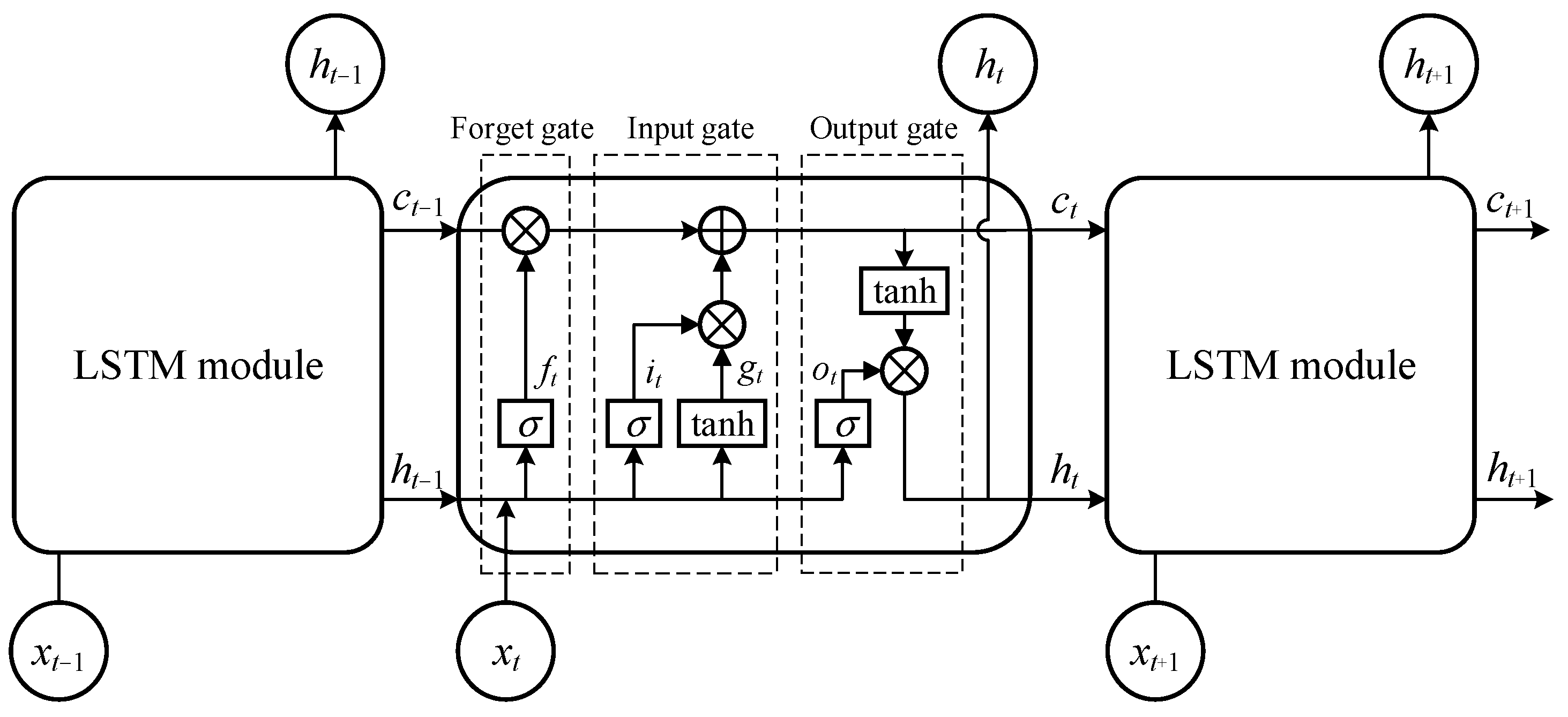
Conventional RNNs have limited ability to capture long-term dependencies due to issues with vanishing or exploding gradients during training lengthy sequences. To address this problem, the long short-term memory network (LSTM) was developed as a specialized type of RNN [28,29]. The LSTM has been widely used for processing sequential data and has found application in various domains of vehicle emission prediction. As shown in Figure 2, the LSTM is equipped with three unique “gate” structures within the neurons. These “gate” structures enable the addition and removal of information, facilitating the flow of states for long-term memory retention. Each LSTM cell contains three “gate” structures: input gate it, forget gate ft, and output gate ot to manage the flow of information.
The forget gate ft determines the information to be discarded and the information to be retained using a sigmoid function that takes the input xt, output from the previous unit ht−1, and internal state outputs. It can be presented by
f t = σ ( W f x t + U f h t 1 + V f c t 1 + b f )
The input gate it also uses a sigmoid layer to decide the new information to be added to the cell, and the input gt creates a new state set. The process can be presented by
i t = σ ( W i x t + U i h t 1 + V i c t 1 + b i ) ,
g t = tanh ( W c x t + U c h t 1 + b c ) .
The output gate ot, determined by a sigmoid layer, produces the cell output ht. The process can be presented by
o t = σ ( W o x t + U o h t 1 + V o C t + b o ) ,
h t = o t tanh ( c t ) ,
where W, U, and V are the parameter matrices, b is the bias, is the element-wise multiplication, σ(·) and tanh(·) are the activation functions, and the subscript t denotes the cell state at time t. Thus, the LSTM is designed to retain useful information for a long time while discarding irrelevant information quickly.

2.3. Dropout for Neural Networks

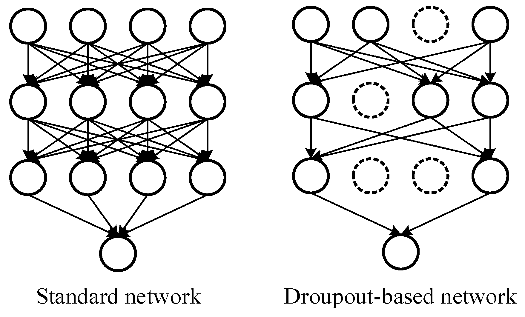
Overfitting is an important problem in multilayer LSTM models. Multilayer LSTM model training and learning is essentially optimization and generalization. Debugging the multilayer LSTM model parameters minimizes the loss function value in the training sample set. The performance of a fully trained predictive model in the test sample set reflects the model’s generalization capabilities. Overfitting can affect the training model’s performance and thus reduce generalization. To prevent models such as multilayer LSTM neural networks from overfitting the training sample set, regularization techniques are adopted to limit the complexity of the model. A regularization term for the model parameters is added to the objective function. The dropout method is one of the most effective regularization tools for deep learning [30], and the standard network and the dropout-based network are shown in Figure 3.

2.4. Loss Function and Optimization

The loss function is a mathematical tool employed to measure the difference between the output value of the neural network and the actual value, which is essential for evaluating the accuracy of the model’s predictions. The specific formulation of the loss function for LSTM is presented as follows:
F l o s s = 1 m t = 1 m y ˜ ( t ) y ( t ) 2 ,
where y ˜ ( t ) is the predicted value, and y(t) is the measured value.
The optimization of the LSTM training process is to obtain the system parameters that can minimize the loss function by iteration. Neural network optimizers are tools used to minimize the loss function by adjusting parameters. Common optimizers include Stochastic Gradient Descent (SGD), momentum optimizer, the Adaptive Gradient Algorithm (AdaGrad), Root Mean Square prop (RMSprop), and Adaptive Moment Estimation (Adam). The Adam optimizer combines momentum and RMSprop, providing adaptive learning rates and momentum adjustments. It adjusts the learning rates for each parameter by computing first- and second-moment estimates of the gradient. Adam converges faster and demonstrates good generalization, making it widely used in practice.

3. Data Preprocessing

Emissions data preprocessing was used to eliminate the data anomalies caused by equipment malfunctions and sensor anomalies. In addition, it helps to make the data more standardized, which is essential for the study of emission prediction models for construction machinery.

3.1. Data Compensation

Due to sensor failures or partial data loss during monitoring, the recorded emission data in the monitoring system are incomplete. Some data are lost during the data transmission and updating process. Therefore, it is necessary to compensate for the missing data before analyzing the emission data. Compensating for incomplete data records could significantly enhance the prediction performance. The process of compensating for missing data mainly consists of three steps:
(1)
Perform data inspection on the original data sequence L to identify the positions of missing data points (xi, yi).
(2)
Select the key data points of (x1, y1) and (x2, y2) nearest to the missing value (xi, yi) from the data sequence L, and perform linear interpolation using these two points. Subsequently, add this interpolated data point (x’i, y’i) to the data sequence L to replace (xi, yi), resulting in an updated dataset L’. The coordinates of the updated data points are as follows:
x i = x i ,
y i = y 1 + y 2 y 1 x 2 x 1 x i x 1 ,
(3)
Repeat steps (1) and (2) until there are no incomplete data points in data sequence L.

3.2. Outlier Detection

The emissions data of off-road construction machinery typically exhibit strong non-stationarity, which may stem from various factors such as varying operating conditions, mechanical wear and tear, differences in fuel quality, maintenance practices, and environmental influences. In addition, frequent acceleration, deceleration, and aerodynamics often put the engine in transient operating conditions. Due to the non-stationarity of the emissions data, selecting appropriate outlier detection methods is crucial. Techniques like local linear regression can better adapt to the non-stationarity of the data, thereby enhancing the accuracy and reliability of outlier detection.
Local linear regression is a non-parametric regression method that, in making predictions, takes into account the local data points surrounding each data point to fit a local linear model. This approach enables the more effective capture of the local characteristics and nonlinear relationships present in the data. Quadratic local linear regression is a variant of local linear regression that fits a quadratic polynomial model around local data points to capture the nonlinear relationships in the data and improve the data quality and analysis reliability. The model for quadratic local linear regression can be presented as follows:
y ^ i   = β 0 ( x i ) + β 1 ( x i ) ( x x i ) + β 2 ( x i ) ( x x i ) 2 + ϵ i ,
where y ^ i is the response variable of the i-th data point, xi is the predictor variable of the i-th data point, β0(xi), β1(xi), and β2(xi) are the local quadratic linear coefficients at xi, and ϵi is the error term.
The objective of quadratic local linear regression is to minimize the following local weighted square error:
m i n i = 1 n w i ( y i β 0 ( x i ) β 1 ( x i ) ( x x i ) β 2 ( x i ) ( x x i ) 2 ) 2 ,
where wi is a weight function that adjusts the influence of each data point during the fitting process, which can be defined using Gaussian or triangular kernel functions. After the iterative parameter adjustments, the optimal fitting model is derived for prediction and analysis.

3.3. Normalization

The emission data were normalized to ensure that all features were on the same scale. Normalization ensures smooth training and not performing normalization might also cause a vanishing gradient problem while training out the LSTM Network. Min–max normalization has been used for normalizing the data. The formula for min–max normalization is as follows:
y i j = x i j min ( x ) max ( x ) min ( x ) ,
where x i j is the j-th feature value of the i-th input sample and y i j is the corresponding normalized value.

4. LSTM-Based Emissions Forecasting Model

The transient emission concentration from off-road construction machinery can vary significantly due to the dynamic and unpredictable nature of construction sites. Factors such as load variations, speed changes, and idling periods contribute to irregular patterns and sudden changes in emission concentrations, making accurate prediction challenging. The complexity of predicting emissions also lies in capturing the intricate nonlinear relationships among factors like the engine load, operating conditions, fuel quality, and environmental influences. The non-stationary nature of emission data further complicates prediction efforts, as traditional models may struggle to adapt to the rapid changes and irregular patterns inherent in off-road machinery emissions.
Deep learning techniques for predicting emission concentrations from off-road machinery offer notable advantages over traditional methods. Deep learning models excel in automatically learning complex features, capturing nonlinear relationships, handling temporal dynamics, scaling with data size, and adapting to changing patterns. These capabilities enable deep learning models to effectively capture the dynamic and non-stationary nature of emission concentration variations, facilitating the accurate predictions crucial for enhancing environmental monitoring and management practices in off-road settings.
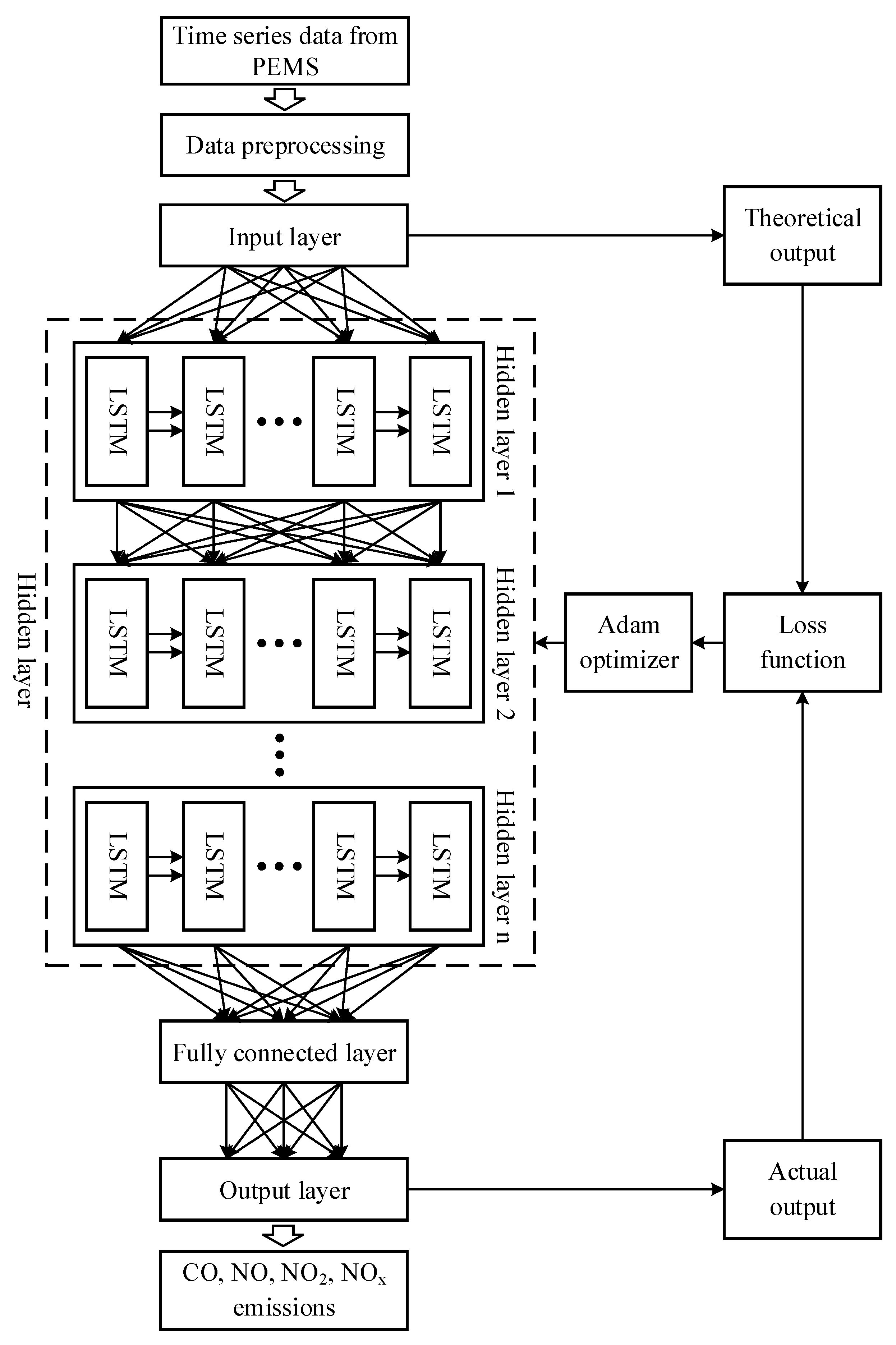
The emission prediction model for off-road construction machinery is shown in Figure 4. The LSTM network used in this research includes one input layer, n hidden layers, and one fully connected output layer. To improve the prediction accuracy, the Adam optimization algorithm is implemented to optimize the LSTM model. Moreover, dropouts are set after each hidden layer to prevent over-fitting. The activation functions of the hidden layer are the sigmoid and tanh functions, and the activation function of the output layer is the linear function.

5. Experimental Results and Discussion

5.1. Data Collection and Setup

Portable emissions measurement systems (PEMSs) can evaluate engine emissions by conducting real-time tests and provide instantaneous emissions, fuel consumption, vehicle speed, temperature, and other parameters based on the equipment capabilities. The data obtained from the analysis of engine exhaust gases by various analyzers within PEMS, in conjunction with environmental and GPS parameters, are input into the data acquisition system and ultimately recorded and stored in a PC. The process of exhaust gas sampling and data processing by PEMS is shown in Figure 5.
An off-road construction machinery dataset was collected and compiled to train and evaluate the proposed model. The dataset was created using PEMS data collected from 19 pieces of off-road machinery in four different types of construction vehicles. The datasets were divided into training and test sets in a 6:2:2 ratio, as shown in Table 1. The ten input features, which are F1, F2, …, and F10, and four output features, which are F11, F12, F13, and F14, are given in Table 2. The LSTM-based emission prediction model was developed using MATLAB R2022b, and detailed information on the experimental environment is shown in Table 3.

5.2. Correlation Analysis

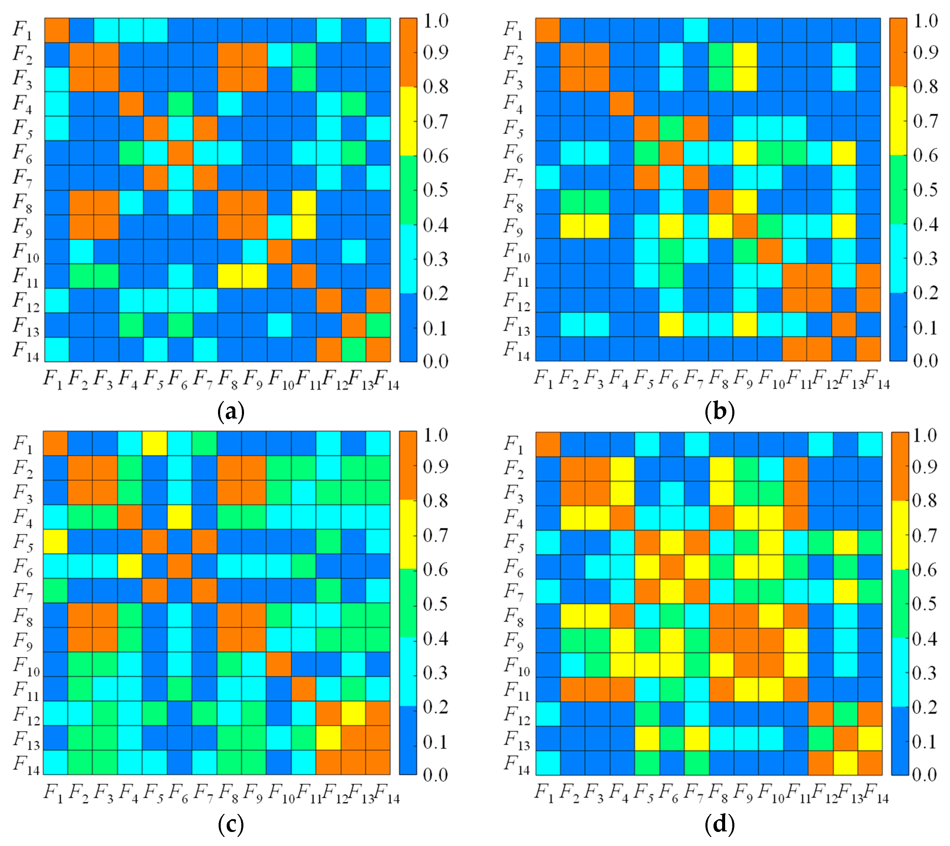
The input features of the time series are expected to be highly correlated with the output results, while the multiple input features are expected to have a low correlation with each other. The absolute value of the Pearson correlation coefficient (|r|) is used to show the correlation between the input and output features. These correlation results are shown in Figure 6. As depicted in Figure 6, the autocorrelation coefficient of each feature is 1.

5.3. Parameter Settings and Evaluation Metrics

The performance and complexity of an LSTM model are directly affected by its hyperparameters, as shown in Table 4. These hyperparameters include the initial learning rate, minimum batch size, number of hidden layers, number of hidden units, and validation frequency. The batch size and the number of learning epochs influence the efficiency of model training. A thorough search using training and validation data is performed to ensure that the hidden layers can capture intricate details and align with the computational capabilities of the system. An LSTM model with three hidden layers and 256 neurons in each layer is found to be the optimal architecture. After evaluating various learning rates and monitoring changes in the iteration times and loss, a learning rate of 0.001 is selected. In the hyperparameter optimization process, the number of epochs is set to 500 to enhance accuracy. A dropout rate of 0.2 in each hidden layer is added to the LSTM model to ensure that the nodes are trained equally.
To assess the effect of the proposed method on predicting off-road machinery emissions, three distinct quantitative evaluation metrics were employed: the root mean squared error (RMSE), mean absolute error (MAE), and mean absolute percentage error (MAPE). These metrics were calculated as follows:
RMSE = 1 N t = 1 N [ y ( t )   y ^ ( t ) ] 2 ,
MAE = 1 N t = 1 N y ( t ) y ^ ( t ) ,
MAPE = 1 N t = 1 N y ( t ) y ^ ( t ) y ( t ) × 100 % .
where y(t) is the true value, y ^ ( t ) is the predicted value, and N is the number of samples for the test set.

5.4. Emissions Prediction for Four Types of Construction Machinery

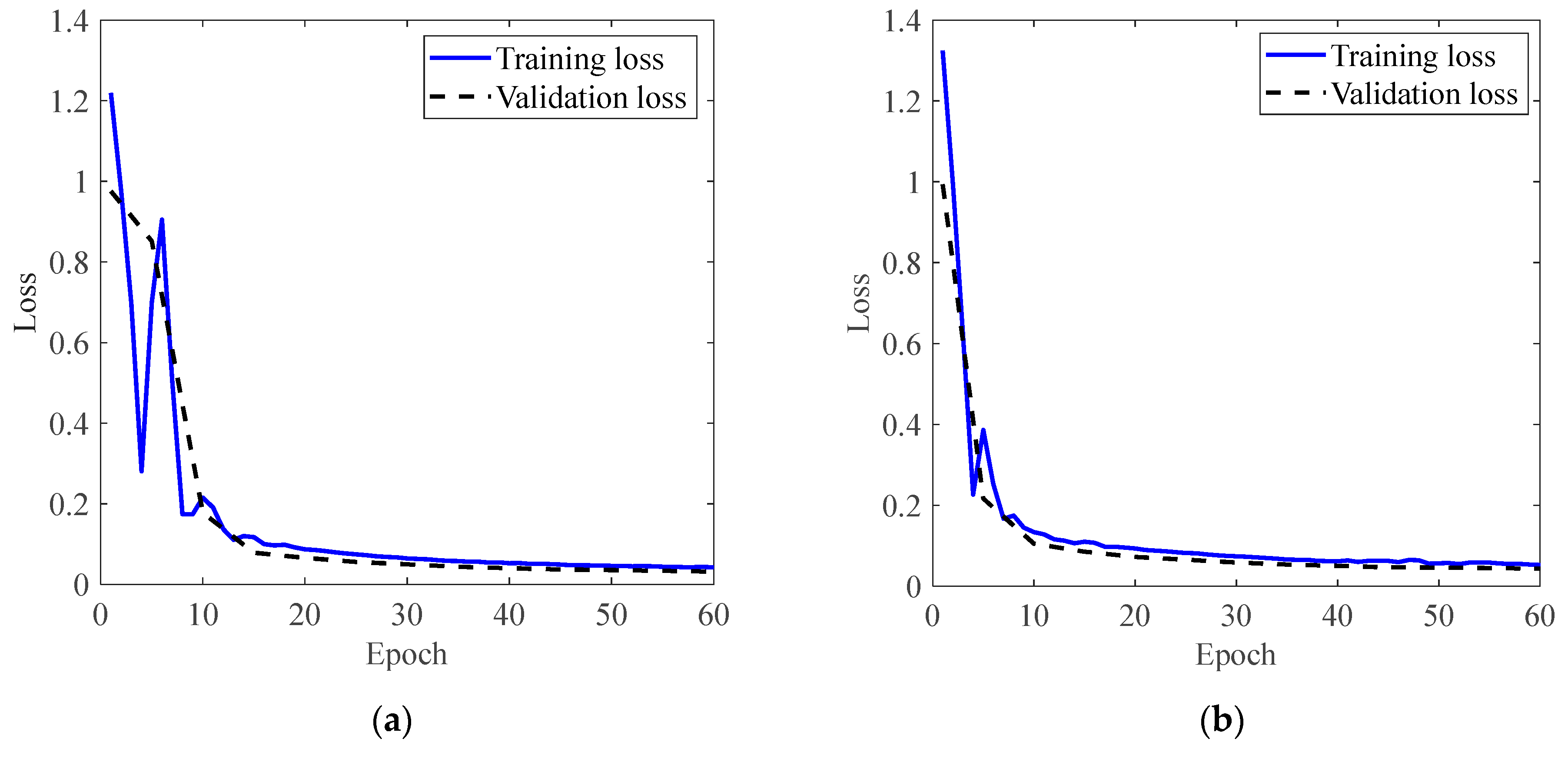
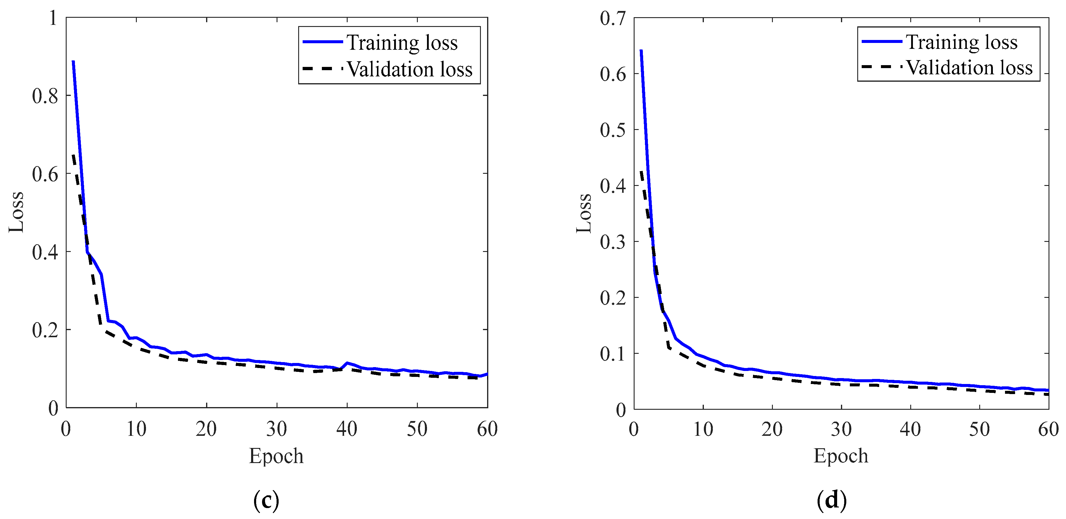
The PEMS test data from four different types of off-road construction vehicles were utilized to train and analyze using the method presented in this paper. Figure 7 shows the training and validation losses of the proposed model with a loss function. The LSTM models for forklifts, loaders, tractors, and forklifts reached their minimum training losses at the 50th, 40th, 60th, and 40th epoch, respectively, while achieving their minimum validation losses at the 40th, 40th, 60th, and 60th epoch, respectively. These results indicate that the final models were not over-fitted, and their accuracies were optimized.
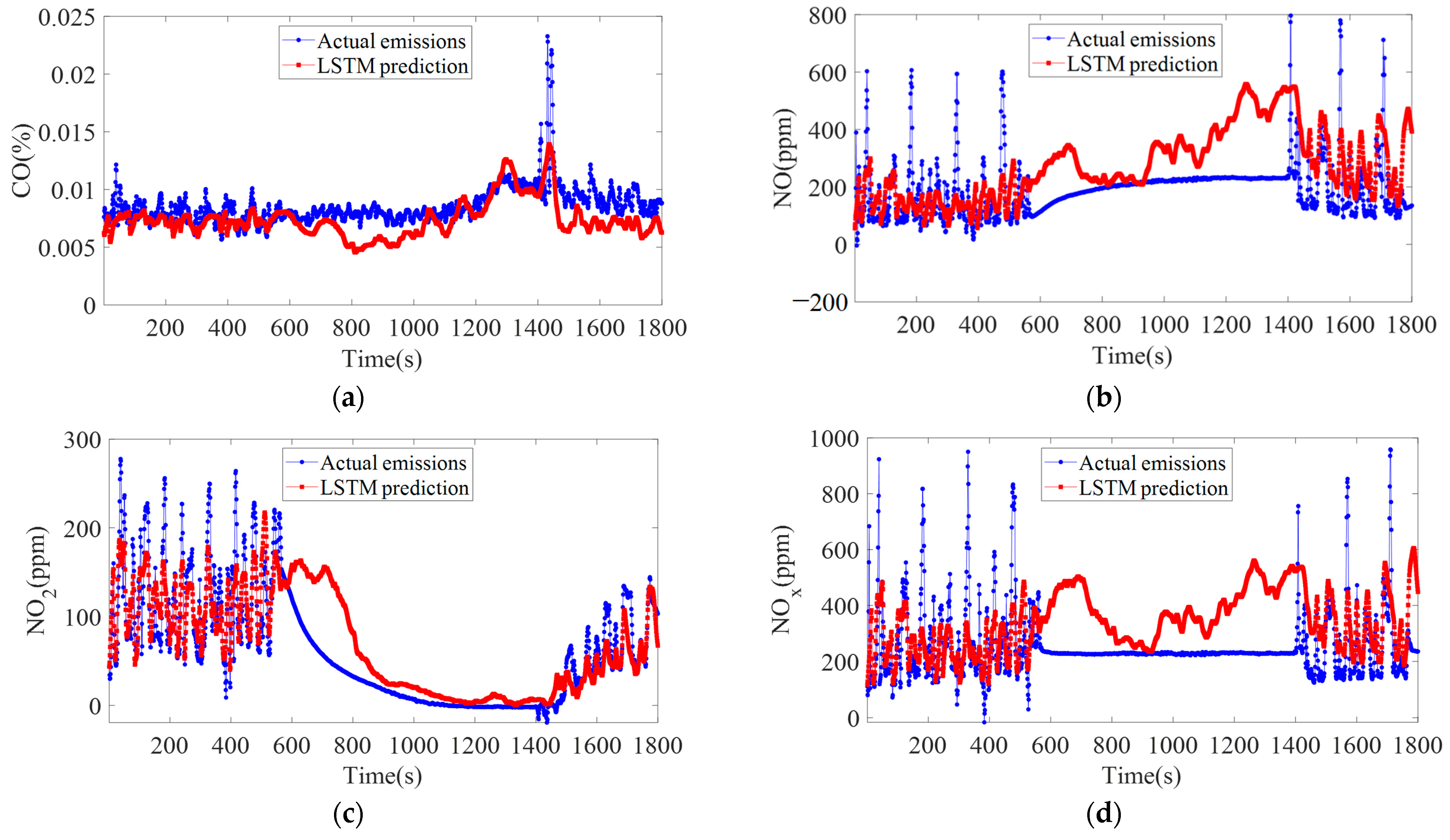
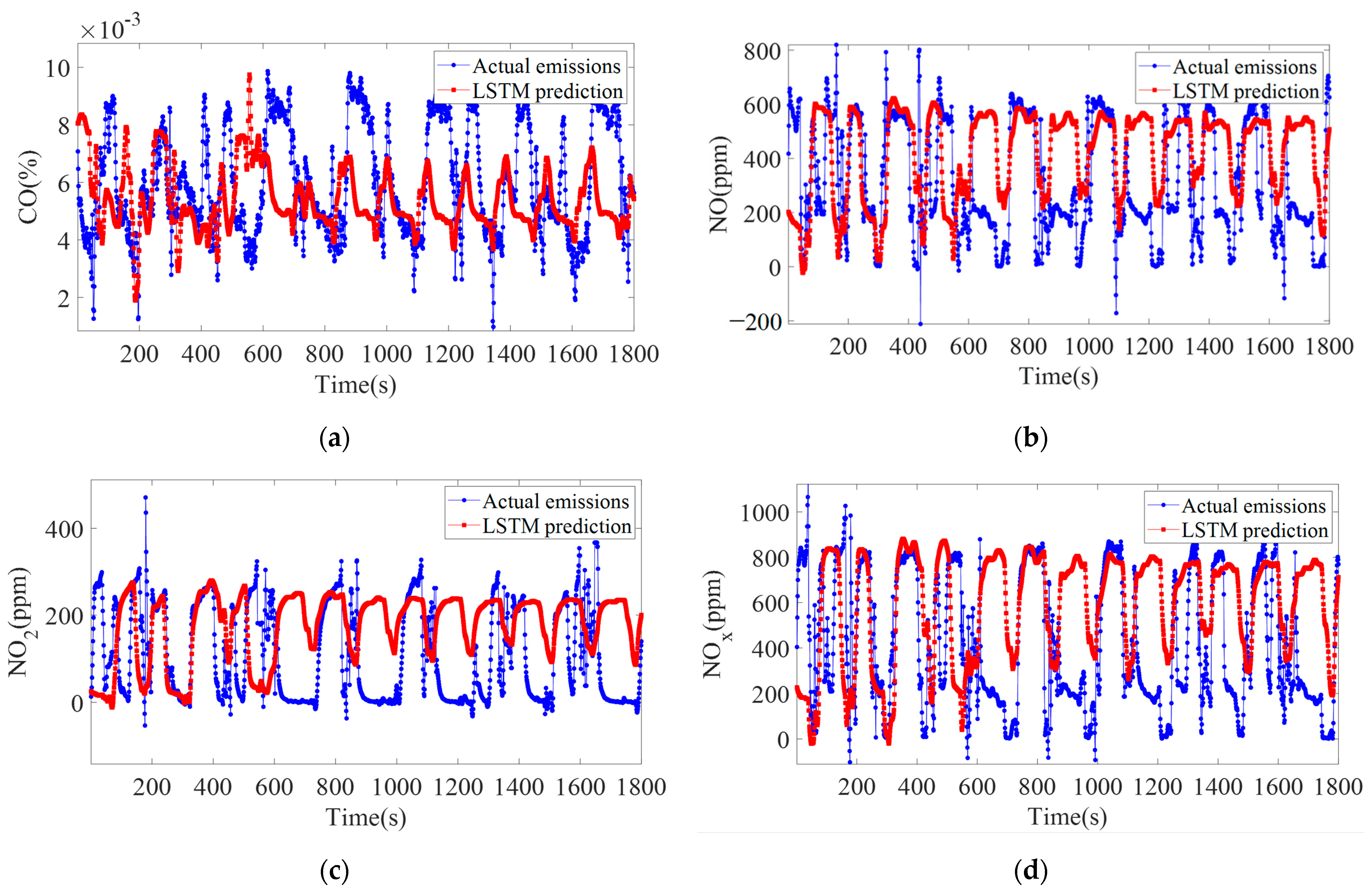
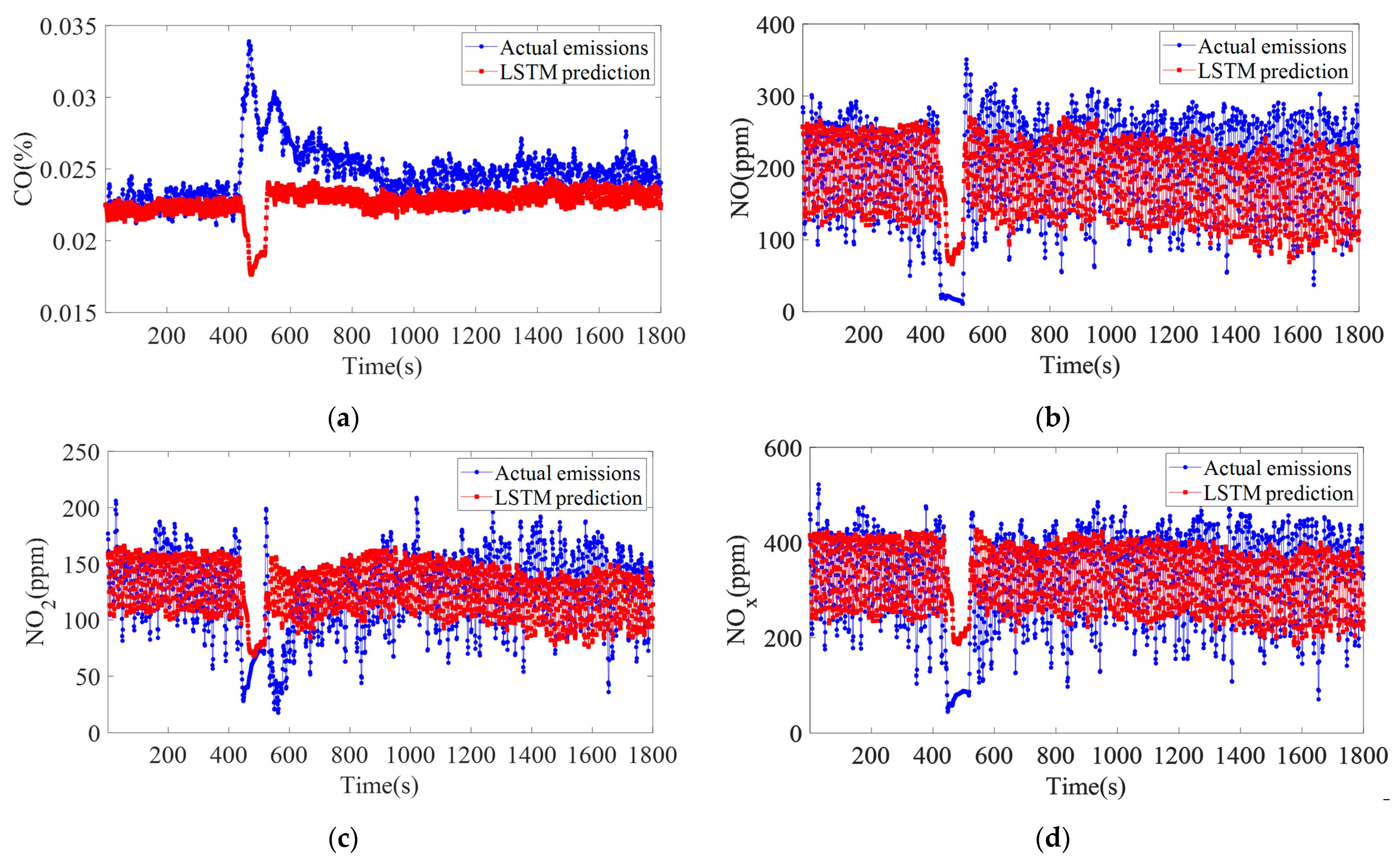
The LSTM neural network model trained on the training set was evaluated for its predictive accuracy on the test set, as depicted in Figure 8, Figure 9, Figure 10 and Figure 11. These figures illustrate comparisons between the experimental and predicted results for the four types of off-road construction machinery in the testing set.
Figure 8 shows the analysis results of the LSTM model on the forklift test set, demonstrating the model’s ability to effectively forecast the emission concentrations of CO, NO, NO2, and NOX under transient conditions with high prediction accuracy. Figure 9 and Figure 10 present the LSTM model predictions of the CO, NO, NO2, and NOX emission concentrations on the loader and tractor test sets. It is noteworthy that the proposed model exhibits a certain level of predictive accuracy even for scenarios with excessively rapid transient changes, albeit with a slightly reduced accuracy compared to the other three types of off-road machinery, as shown in the analysis results for the excavator in Figure 11. This phenomenon is understandable as LSTM networks may struggle with capturing long-term dependencies when dealing with non-stationary data, given the sudden fluctuations in and volatility of the data. The results indicate the effectiveness of the proposed LSTM emission prediction model for off-road machinery under various operating conditions, and its ability to provide accurate predictions even in the presence of challenging transient conditions.
Table 5 shows the performance indicators of the proposed LSTM emission prediction model. It can be noticed that the loader has the highest RMSE, while the forklift has the lowest RMSE for CO, NO, NO2, and NOx emission forecasting. When forecasting the NO emissions of the four off-road construction machinery, the forklift has a high RMSE of 143.6624, much higher than the 56.3650 of the loader. Table 5 also confirms the prediction accuracy of the LSTM model in terms of MAE and MAPE. Considering the three indicators of RMSE, MAE, and MAPE comprehensively, it can be observed that the proposed model performs the best when predicting the emissions for loaders and the worst when predicting the emissions for tractors. From the trend in the emissions data for tractors, it can be inferred that the reason for this may be that the concentration of emissions fluctuates significantly. Overall, the proposed LSTM-based emission prediction model can reasonably forecast the exhaust emission concentrations of various types of off-road construction machinery.

5.5. Discussion

In Table 6, the proposed method is compared with other approaches. It can be seen that by employing an LSTM model and leveraging PEMS data for off-road vehicles, the current method not only provides a long period of 30 min of prediction for a variety of pollutants such as CO, NO, NO2, and NOX, but also addresses the unique challenges associated with off-road environments. The findings underscore the potential of the proposed method to offer robust and actionable insights for emission control and policy making in sectors that extensively use off-road machinery.
It should also be noted that the vibration of construction machinery significantly contributes to dust dispersion. The proposed LSTM model can be further enhanced to explore the mechanisms of dust generation and improve the model’s predictive accuracy.

6. Conclusions

A long short-term memory network model is proposed to predict the emission of CO, NO, NO2, and NOx from four kinds of off-road construction machinery. The model considers nine input features, which are the vehicle speed, ambient temperature, ambient relative humidity, emission flow rate, emission temperature, and emission pressure differential. The predicted results of the model are CO, NO, NO2, and NOx. When some emission data samples are incomplete, a method based on linear interpolation is used to compensate for the missing data. Local linear regression is applied to smooth the raw emission time series, which exhibit strong non-stationary characteristics, and to detect outliers. For each outlier, a local linear fit is used to update the database. The preprocessed data are then input into the proposed LSTM model to obtain the emission concentrations of CO, NO, NO2, and NOx. The emission data measured using a portable emission measurement system are used to train the proposed LSTM-based emission prediction model, and the predicted results are compared with the experimental results of four types of off-road construction machinery, including a forklift, loader, tractor, and excavator. The experimental results show that the proposed LSTM-based model can predict the emission concentrations of different off-road construction machinery under transient operating conditions.

Author Contributions

Conceptualization, T.L., X.J., F.W., X.W., D.G., X.C. and B.T.; methodology, T.L., X.J., F.W., X.W., D.G., X.C. and B.T.; software, T.L., X.J., F.W., X.W., D.G., X.C. and B.T.; investigation, T.L., X.J., F.W., X.W., D.G., X.C. and B.T.; data curation, T.L., X.J., F.W., X.W., D.G., X.C. and B.T.; writing—original draft preparation, T.L., X.J., F.W., X.W., D.G., X.C. and B.T.; writing—review and editing, T.L., X.J., F.W., X.W., D.G., X.C. and B.T. All authors have read and agreed to the published version of the manuscript.

Funding

This research received no external funding.

Data Availability Statement

The original contributions presented in the study are included in the article, further inquiries can be directed to the corresponding author.

Conflicts of Interest

Authors Tengteng Li, Xiaojun Jing, Fengbin Wang, Xiaowei Wang and Dongzhi Gao were employed by the company CATARC Automotive Test Center Co., Ltd. The remaining authors declare that the research was conducted in the absence of any commercial or financial relationships that could be construed as a potential conflict of interest.

References

  1. Chan, C.K.; Yao, X. Air pollution in mega cities in China. Atmos. Environ. 2008, 42, 1–42. [Google Scholar] [CrossRef]
  2. Weschler, C.J. Ozone’s impact on public health: Contributions from indoor exposures to ozone and products of ozone-initiated chemistry. Environ. Health Perspect. 2006, 114, 1489–1496. [Google Scholar] [CrossRef]
  3. Bakay, M.S.; Agbulut, Ü. Electricity production based forecasting of greenhouse gas emissions in Turkey with deep learning, support vector machine and artificial neural network algorithms. J. Clean Prod. 2021, 285, 125324. [Google Scholar] [CrossRef]
  4. Ministry of Ecology and Environment of the People’s Republic of China. China Mobile Source Environmental Management Annual Report; Ministry of Ecology and Environment (MEE): Beijing, China, 2019. (In Chinese) [Google Scholar]
  5. Wang, Y.Q.; Yin, W.; Yan, Q.Z.; Cheng, Y. Emission characteristics of particulate matter emitted by typical off-road construction machinery, Environ. Sci. Pollut. Res. 2022, 29, 44220–44232. [Google Scholar] [CrossRef] [PubMed]
  6. Ministry of Ecology and Environment of the People’s Republic of China. China Mobile Source Environmental Management Annual Report; Ministry of Ecology and Environment (MEE): Beijing, China, 2021. (In Chinese) [Google Scholar]
  7. Goldberg, D.L.; Harkey, M.; de Foy, B.; Judd, L.; Johnson, J.; Yarwood, G.; Holloway, T. Evaluating NOx emissions and their effect on O3 production in Texas using TROPOMI NO2 and HCHO. Atmos. Chem. Phys. 2022, 22, 10875–10900. [Google Scholar] [CrossRef]
  8. Liu, Z.Q.; Li, D.F.; Zhang, J.E.; Saleem, M.; Zhang, Y.; Ma, R.; He, Y.N.; Yang, J.Y.; Xiang, H.M.; Wei, H. Effect of simulated acid rain on soil CO2, CH4 and N2O emissions and microbial communities in an agricultural soil. Geoderma 2020, 366, 114222. [Google Scholar] [CrossRef]
  9. Hou, X.N.; Tian, J.L.; Song, C.B.; Wang, J.; Zhao, J.Y.; Zhang, X.M. Emission inventory research of typical agricultural machinery in Beijing, China. Atmos. Environ. 2019, 216, 116903. [Google Scholar] [CrossRef]
  10. Tu, R.; Li, T.Z.; Meng, C.S.; Chen, J.Y.; Sheng, Z.; Xie, Y.S.; Xie, F.J.; Yang, F.; Chen, H.B.; Li, Y.; et al. Real-world emissions of construction mobile machines and comparison to a non-road emission model. Sci. Total Environ. 2021, 771, 145365. [Google Scholar] [CrossRef]
  11. Jaworski, A.; Kuszewski, H.; Ustrzycki, A.; Balawender, K.; Lejda, K.; Wos, P. Analysis of the repeatability of the exhaust pollutants emission research results for cold and hot starts under controlled driving cycle conditions, Environ. Sci. Pollut. Res. 2018, 25, 17862–17877. [Google Scholar] [CrossRef]
  12. Geller, V.D.; Sardar, S.B.; Phuleria, H.; Fine, P.N.; Sioutas, C. Measurements of particle number and mass concentrations and size distributions in a tunnel environment, Environ. Sci. Technol. 2005, 39, 8653–8663. [Google Scholar] [CrossRef]
  13. Xie, H.; Zhang, Y.; He, Y.; You, K.; Fan, B.Q.; Yu, D.Q.; Li, M.Q. Automatic and fast recognition of on-road high-emitting vehicles using an optical remote sensing system. Sensors 2019, 19, 3540. [Google Scholar] [CrossRef] [PubMed]
  14. Bishop, G.A.; Peddle, A.M.; Stedman, D.H.; Zhan, T. On-road emission measurements of reactive nitrogen compounds from three California cities, Environ. Sci. Technol. 2010, 44, 3616–3620. [Google Scholar] [CrossRef] [PubMed]
  15. O’Driscoll, R.; ApSimon, H.M.; Oxley, T.; Molden, N.; Stettler, M.E.J.; Thiyagarajah, A. A portable emissions measurement system (PEMS) study of NOx and primary NO2 emissions from euro 6 diesel passenger cars and comparison with COPERT emission factors. Atmos. Environ. 2016, 145, 81–91. [Google Scholar] [CrossRef]
  16. Frey, H.C.; Rasdorf, W.; Lewis, P. Comprehensive field study of fuel use and emissions of nonroad diesel construction equipment. Transp. Res. Record 2010, 2158, 69–76. [Google Scholar] [CrossRef]
  17. Ropkins, K.; DeFries, T.H.; Pope, F.; Green, D.C.; Kemper, J.; Kishan, S.; Fuller, G.W.; Li, H.; Sidebottom, J.; Crilley, L.R.; et al. Evaluation of EDAR vehicle emissions remote sensing technology. Sci. Total Environ. 2017, 609, 1464–1474. [Google Scholar] [CrossRef] [PubMed]
  18. Heidari, B.; Marr, L.C. Real-time emissions from construction equipment compared with model predictions. J. Air Waste Manag. Assoc. 2015, 65, 115–125. [Google Scholar] [CrossRef] [PubMed]
  19. Singh, M.; Dubey, R.K. Deep learning model based CO2 emissions prediction using vehicle telematics sensors data. IEEE Trans. Intell. Veh. 2023, 8, 768–777. [Google Scholar] [CrossRef]
  20. Yu, Y.; Wang, Y.Y.; Li, J.Q.; Fu, M.L.; Shah, A.N.; He, C. A novel deep learning approach to predict the instantaneous NOx emissions from diesel engine. IEEE Access 2021, 9, 11002–11013. [Google Scholar] [CrossRef]
  21. Shin, S.; Lee, Y.; Park, J.; Kim, M.; Lee, S.; Min, K. Predicting transient diesel engine NOx emissions using time-series data preprocessing with deep-learning models. Proc. Inst. Mech. Eng. Part D J. Automob. Eng. 2021, 235, 3170–3184. [Google Scholar] [CrossRef]
  22. Zhang, Q.; Li, F.; Long, F.; Ling, Q. Vehicle emission forecasting based on wavelet transform and long short-term memory network. IEEE Access 2018, 6, 56984–56994. [Google Scholar] [CrossRef]
  23. Zhang, R.S.; Wang, Y.G.; Pang, Y.J.; Zhang, B.W.; Wei, Y.B.; Wang, M.L.; Zhu, R.C. A deep learning micro-scale model to estimate the CO2 emissions from light-duty diesel trucks based on real-world driving. Atmosphere 2022, 13, 1466. [Google Scholar] [CrossRef]
  24. Xie, H.; Zhang, Y.; He, Y.; You, K.; Fan, B.Q.; Yu, D.Q.; Lei, B.; Zhang, W.C. Parallel attention-based LSTM for building a prediction model of vehicle emissions using PEMS and OBD. Measurement 2021, 185, 110074. [Google Scholar] [CrossRef]
  25. Shi, Z.; Shi, M.; Li, C. The prediction of character based on recurrent neural network language model. In Proceedings of the 2017 IEEE/ACIS 16th International Conference on Computer and Information Science (ICIS), Wuhan, China, 24–26 May 2017. [Google Scholar]
  26. Zhang, X.Y.; Yin, F.; Zhang, Y.M.; Liu, C.L.; Bengio, Y. Drawing and recognizing Chinese characters with recurrent neural network. IEEE Trans. Pattern Anal. Mach. Intell. 2018, 40, 849–862. [Google Scholar] [CrossRef] [PubMed]
  27. Guo, L.; Li, N.P.; Jia, F.; Lei, Y.G.; Lin, J. A recurrent neural network based health indicator for remaining useful life prediction of bearings. Neurocomputing 2017, 240, 98–109. [Google Scholar] [CrossRef]
  28. Zhao, H.; Sun, S.; Jin, B. Sequential fault diagnosis based on LSTM neural network. IEEE Access 2018, 6, 12929–12939. [Google Scholar] [CrossRef]
  29. Song, H.; Dai, J.J.; Luo, L.G.; Sheng, G.H.; Jiang, X.C. Power transformer operating state prediction method based on an LSTM network. Energies 2018, 11, 914. [Google Scholar] [CrossRef]
  30. Yang, G.T.; Wang, Y.N.; Li, X.L. Prediction of the NOx emissions from thermal power plant using long short term memory neural network. Energy 2020, 192, 116597. [Google Scholar] [CrossRef]
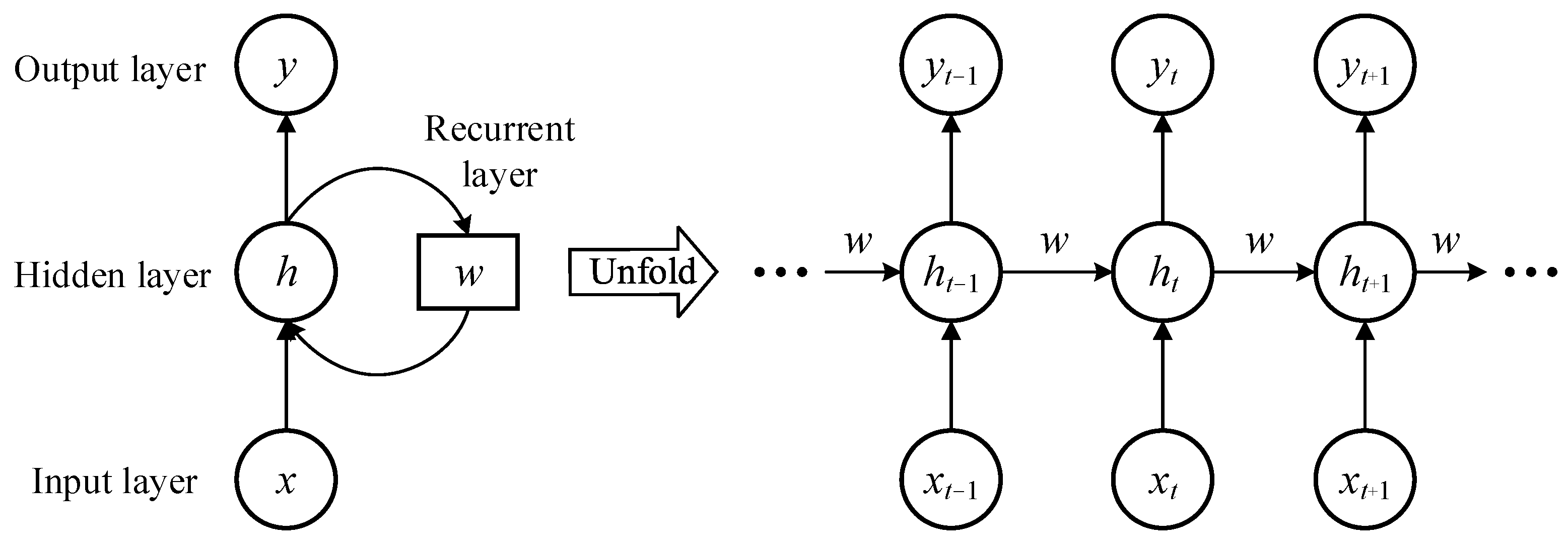
Figure 1. Structural diagram of the RNN.
Energies 17 03373 g001
Figure 2. Structural diagram of the LSTM.
Energies 17 03373 g002
Figure 3. Diagram of the standard network and dropout network. The dotted circles indicate neurons that are randomly deactivated with a certain probability.
Energies 17 03373 g003
Figure 4. LSTM-based emissions forecasting model.
Energies 17 03373 g004
Figure 5. The schemes follow the same formatting.
Energies 17 03373 g005
Figure 6. Correlation analysis results of four types of off-road construction machinery: (a) forklift; (b) loader; (c) tractor; (d) excavator.
Energies 17 03373 g006
Figure 7. Training and validation losses according to the epoch: (a) forklift; (b) loader; (c) tractor; (d) excavator.
Energies 17 03373 g007aEnergies 17 03373 g007b
Figure 8. Emission prediction results of a forklift using the LSTM model: (a) CO; (b) NO; (c) NO2; (d) NOX.
Energies 17 03373 g008
Figure 9. Emission prediction results of a loader using the LSTM model: (a) CO; (b) NO; (c) NO2; (d) NOX.
Energies 17 03373 g009
Figure 10. Emission prediction results of a tractor using the LSTM model: (a) CO; (b) NO; (c) NO2; (d) NOX.
Energies 17 03373 g010
Figure 11. Emission prediction results of an excavator using the LSTM model: (a) CO; (b) NO; (c) NO2; (d) NOX.
Energies 17 03373 g011
Table 1. Experimental datasets.
DatasetsSize
TrainingValidationTestTotal
Forklift5794193119319656
Loader5629187718779383
Tractor4594153115317656
Excavator4415147214727359
Table 2. Input data and output data of the LSTM model.
Symbol (Units)Description
Input dataF1 (km/h)Vehicle speed
F2 (°C)Ambient temperature
F3 (%)Ambient relative humidity
F4 (kPa)Atmospheric pressure
F5 (m3/min)Emission flow rate
F6 (°C)Emission temperature
F7 (Pa)Emission pressure differential
F8 (°C)Analyzer temperature
F9 (°C)Exhaust pipe ambient temperature
F10 (%)Exhaust pipe ambient absolute humidity
Output dataF11 (%)CO
F12 (ppm)NO
F13 (ppm)NO2
F14 (ppm)NOx
Table 3. Experimental environment.
ParametersValue
CPUInter(R) Core (TM) i7-10875H CPU @ 2.30 GHz
GPUNVIDIA GeForce RTX 2060
Number of GPU cards1
Memory (RAM, VRAM)16.0, 6.0 GB
Table 4. Parameter setting of the LSTM model.
LSTM ParametersValue
Initial learning rate0.001
Learning rate drop period125
Learning rate drop factor0.2
Validation frequency5
Minimum batch size10
Maximum epochs500
Gradient threshold1
Number of hidden layers2
Number of hidden units256
Dropout rate0.2
Table 5. Performance indicators of the LSMT emission prediction model.
EmissionsRMSEMAEMAPE
ForkliftCO0.00170.00140.1541
NO143.6624111.49380.6676
NO235.875825.18913.4717
NOx164.1304131.67800.5866
LoaderCO376.9817318.827154.8420
NO56.365041.82540.2550
NO250.222637.96450.2319
NOx87.269265.72380.1958
TractorCO0.00230.00180.3149
NO245.4075199.68047.3622
NO2152.0607124.355948.3758
NOx371.7461291.26635.9550
ExcavatorCO0.00300.00200.07600
NO46.710936.29140.3589
NO228.674521.14960.2393
NOx66.999750.67440.2456
Table 6. Comparison of different emission forecasting methods.
ReferencesVehicle TypeDeep Learning ModelsData AcquisitionForecasting Time (min)Forecasted Emissions
Singh et al. [19]On-roadLSTMOBD400CO2
Yu et al. [20]On-roadLSTMOBD33NOX
Shin et al. [21]N/ADNN & LSTMFast analyzer30NOX
Zhang et al. [22]On-roadWavelet + LSTMMonitoring System180CO, HC, NO
Zhang et al. [23]On-roadLSTMPEMS20CO2
Xie et al. [24]N/ALSTMPEMS + OBD175CO, NO, NO2, THC
This studyOff-roadLSTMPEMS30CO, NO, NO2, NOX
Disclaimer/Publisher’s Note: The statements, opinions and data contained in all publications are solely those of the individual author(s) and contributor(s) and not of MDPI and/or the editor(s). MDPI and/or the editor(s) disclaim responsibility for any injury to people or property resulting from any ideas, methods, instructions or products referred to in the content.