Article

Sequential Data-Based Fault Location for Single-Line-to-Ground Fault in a T-Connection Power Line

1
State Grid Shandong Electric Power Research Institute, Jinan 250003, China
2
Shandong Smart Grid Technology Innovation Center, Jinan 250003, China
3
National Key Laboratory of New Power System Operation and Control, Department of Electrical Engineering Tsinghua University, Haidian District, Beijing 100084, China
*
Author to whom correspondence should be addressed.
Energies 2024, 17(12), 2975; https://doi.org/10.3390/en17122975
Submission received: 27 March 2024 / Revised: 23 May 2024 / Accepted: 28 May 2024 / Published: 17 June 2024
(This article belongs to the Topic Power System Protection)

Abstract

:
Due to the demand for temporary rapid grid connection in renewable energy power plants, the topology structure of T-connected power lines has been widely used in the power grid. In this three-terminal system, fault localization is difficult because of traditional impedance-based or traveling wave-based fault localization methods; the three-terminal data should be synchronized and communicated. Since different terminal assets belong to different enterprises, it is actually difficult to maintain good synchronization between them. Therefore, in practical applications, the fault location of T-connected power lines often fails. This article proposes a single terminal fault location method for a T-connection power line to address this issue. It is based on the fact that the local topology of the T-connected power line in the healthy phase remains unchanged during the fault-clearing process. It utilizes the sequential current and voltage data changes generated by the sequential tripping ping emitted by the circuit breaker from different terminals to describe the constant topology of the healthy phase as an equation and calculates the accurate fault location after solving the equation. The Levenberg–Marquardt algorithm was used to calculate fault distance and transition resistance, and the effectiveness of this method was verified through simulation.

1. Introduction

Due to the demand for temporary fast grid connection in renewable power plants (such as wind farms or photovoltaic power stations), the topology structure of T-connected power lines has been widely used in the power grid [1,2]. Even though it is planned and operated as a temporary grid connection mode, it often exists for a long time due to negotiation or other reasons. In this three-terminal system, fault localization is difficult because, for traditional impedance-based or traveling wave-based fault localization methods, the three-terminal fault data should be synchronized and communicated between them [3,4].
However, different terminal assets typically belong to different enterprises and have different maintenance capabilities. For example, after a relatively long operation, the condition of wind farm terminal equipment is usually worse than that of utility terminal equipment. Therefore, due to unstable clock synchronization or other reasons, it is actually difficult to maintain good synchronization between them [5,6]. The traditional fault location method based on three-terminal information sharing cannot be applied.
The fault location method based on single-ended impedance utilizes the linear relationship between fault distance and impedance [7,8]. This method describes and calculates the voltage equation between the meter point and the fault point, thereby obtaining the fault distance. Due to the fact that the number of variables is greater than the number of voltage equations, even on a dual-ended power line, solving the equation is required. We must assume that the equivalent system impedance at the opposite end is known or assume that the phase between the zero-sequence current at the meter point and the zero-sequence current at the fault branch is the same [9,10]. Therefore, the fault location method based on a single impedance cannot theoretically obtain accurate fault distance.
Fortunately, circuit breakers exhibit the ability to trip on a single line in high-voltage power lines. Each trip of any circuit breaker produces voltage and current changes, which can be measured by the relay at the terminal when the last circuit breaker trips [11,12]. Therefore, relays can collect sequential current and voltage data generated by the occurrence of faults and the tripping of circuit breakers in opposite-phase faults. By using sequence data, more equations describing healthy phase lines can be written, and accurate fault distances can be calculated because the number of equations will exceed the number of variables.
Based on the above basic ideas, this article is organized as follows. The section analyzed the sequential voltage and current variation characteristics of all time stages during the entire fault clearance process in Section 2. The simplification of complex equation systems proposed in Section 2 and related solving algorithms can be found in Section 3. The case simulation proves the precise fault localization accuracy in Section 4. The conclusion can be found in Section 5.

2. Sequential Characteristic Analysis of Single-Line-to-Ground Fault in a T-Connection Power Line

Figure 1 shows the topology of a T-shaped connected power system. Assuming a single-line-to-ground fault occurs with resistance R at point F in phase A. The distance between T-connection point P and fault point F is xlN. lM, lN, and lK are the lengths of transmission line sections between bus M and T-connection point P, between bus N and T-connection point P, and between bus K and T-connection point P, respectively. The faulty phase circuit breakers of terminals N and K trip in sequence.
Then, measuring the voltage at point M can collect several sequential data, and the voltage and current at point P can be calculated, as shown in (1) [13].
[ U P 1 s U P 2 s U P 0 s ] = [ U M 1 s U M 2 s U M 0 s ] [ Z c 1 l M Z c 1 l M Z c 0 l M ] [ I M 1 s I M 2 s I M 0 s ]
where U p φ s is voltage phasor; the subscript p presents the location and denotes terminal M, N, K, or T point P or fault point F with value M, N, K, P, or F, respectively. The subscript φ denotes phases A, B, or C with value a, b, or c, and it also can denote positive, negative, or zero sequences with value 1, 2, and 0, respectively. Zc0 and Zc1 are zero sequence and positive sequence wave impedance. I p φ s is current phasor; the superscript s denotes different fault stages. Four stages were defined throughout the entire troubleshooting process. The superscript s is n during normal system operation; f during fault occurrence, without any circuit breaker tripping; and then t after one of the opposite circuit breakers in the fault phase trips. And finally, it takes value i in the stage of the second pair of circuit breakers tripping.
The sequential fault characteristics in three stages after fault occurrence are analyzed as follows.

2.1. The Stage after Fault Occurrence

First, analyze the KP branch; it has
[ U P 1 f U P 2 f U P 0 f ] = [ U K 1 f U K 2 f U K 0 f ] [ Z c 1 l K Z c 1 l K Z c 0 l K ] [ I K 1 f I K 2 f I K 0 f ]
And the boundary condition at point K is presented as follows:
[ E K 0 0 ] = [ U K 1 f U K 2 f U K 0 f ] + [ Z K 1 Z K 1 Z K 0 ] [ I K 1 f I K 2 f I K 0 f ]
where ZK1 and ZK0 are the positive and zero sequence equivalent system impedances at terminal K. Take (3) into (2); the voltage equations between terminal K and point P are shown
{ U P 1 f = E K ( Z K 1 + Z c 1 l K ) I K 1 f U P 2 f = ( Z K 1 + Z c 1 l K ) I K 2 f U P 0 f = ( Z K 0 + Z c 0 l K ) I K 0 f
And then analyze the fault branch NP; it has
[ U F 1 f U F 2 f U F 0 f ] = [ U N 1 f U N 2 f U N 0 f ] + l N ( 1 x ) [ Z c 1 Z c 1 Z c 0 ] [ I N 1 f I N 2 f I N 0 f ]
At fault point F, it has the following boundary conditions:
[ I P N 1 f I P N 2 f I P N 0 f ] = 1 3 [ 1 α α 2 1 α 2 α 1 1 1 ] [ I N a f + U F a f R I N b f I N c f ] = [ I N 1 f + U F a f / ( 3 R ) I N 2 f + U F a f / ( 3 R ) I N 0 f + U F a f / ( 3 R ) ]
U F a f = U F 1 f + U F 2 f + U F 0 f
Therefore, combine (5)–(7); it can present as (8) in branch NP:
[ I P N 1 f I P N 2 f I P N 0 f ] = C [ I N 1 f I N 2 f I N 0 f ] + D [ U N 1 f U N 2 f U N 0 f ]
where D = 1/(3R).
C = l N ( 1 x ) 3 R [ Z c 1 + 3 R l N ( 1 x ) Z c 1 Z c 0 Z c 1 Z c 1 + 3 R l N ( 1 x ) Z c 0 Z c 1 Z c 1 Z c 0 + 3 R l N ( 1 x ) ]
The voltage equation between point F and point P on branch NP is shown as follows:
[ U P 1 f U P 2 f U P 0 f ] = [ U F 1 f U F 2 f U F 0 f ] + l N x [ Z c 1 Z c 1 Z c 0 ] [ I P N 1 f I P N 2 f I P N 0 f ]
Take (5) and (8) into (10); it has
[ U P 1 f U P 2 f U P 0 f ] = A [ U N 1 f U N 2 f U N 0 f ] + B [ I N 1 f I N 2 f I N 0 f ]
where
A = [ Z c 1 l N x 3 R + 1 Z c 1 l N x 3 R Z c 1 l N x 3 R Z c 1 l N x 3 R Z c 1 l N x 3 R + 1 Z c 1 l N x 3 R Z c 0 l N x 3 R Z c 0 l N x 3 R Z c 0 l N x 3 R + 1 ]
B = Z c 1 l N ( x x 2 ) / ( 3 R )   [ 3 R x x 2 + Z c 1 l N Z c 1 l N Z c 0 l N Z c 1 l N 3 R x x 2 + Z c 1 l N Z c 0 l N Z c 0 l N Z c 0 l N Z c 0 3 R ( x x 2 ) Z c 1 + Z c 0 2 l N Z c 1 ]
Similarly, the boundary conditions at terminal N are as follows:
[ E N 0 0 ] = [ U N 1 f U N 2 f U N 0 f ] + [ Z N 1 Z N 1 Z N 0 ] [ I N 1 f I N 2 f I N 0 f ]
Take (14) into (11); the functions between the current on terminal N and the voltage at point P are shown as
[ U P 1 f U P 2 f U P 0 f ] = A [ E N Z N 1 I N 1 f Z N 1 I N 2 f Z N 0 I N 0 f ] + B [ I N 1 f I N 2 f I N 0 f ]
Take (14) into (8); the function among three currents in all three T branches in Figure 1 is shown as
[ I M 1 f I M 2 f I M 0 f ] = [ I K 1 f I K 2 f I K 0 f ] + C [ I N 1 f I N 2 f I N 0 f ] + D [ E N Z N 1 I N 1 f Z N 1 I N 2 f Z N 0 I N 0 f ]
Therefore, the scenario in the stage after fault occurrence can be fully described with Equations (1), (4), (15) and (16). It includes four equations and can generate nine complex equations involving 14 unknown quantities (12 unknown complex quantities EN, ZN1, ZN0, EK, ZK1, ZK0, I N 1 f , I N 2 f , I N 0 f , I K 1 f , I K 2 f , I K 0 f , and 2 unknown real quantities R, x).

2.2. The Stage after One Opposite Terminal (Suppose N Terminal) Circuit Breaker Tripping

The derivation process in this section is similar to the process in section A. Because the topology of branch KP did not change during this stage, the equation in branch KP is the same as in (4), except that the superscript f should be replaced with t, as shown in (17).
{ U P 1 t = E K ( Z K 1 + Z c 1 l K ) I K 1 t U P 2 t = ( Z K 1 + Z c 1 l K ) I K 2 t U P 0 t = ( Z K 0 + Z c 0 l K ) I K 0 t
Since the phase A circuit breaker on terminal N was tripped, the voltage in branch NP can be described as
{ U P a t = ( I M a t + I K 1 t + I K 2 t + I K 0 t ) R + [ Z l s ( I M a t + I K 1 t + I K 2 t + I K 0 t ) + Z l m ( I N b t + I N c t ) ] l N x U P b t = Z l m ( I M a t + I K 1 t + I K 2 t + I K 0 t ) l N x + ( Z l s I N b t + Z l m I N c t ) l N + U N b t U P c t = Z l m ( I M a t + I K 1 t + I K 2 t + I K 0 t ) l N x + ( Z l m I N b t + Z l s I N c t ) l N + U N c t
And the boundary conditions at terminal N is shown as
[ E N α 2 E N α E N ] = [ Z n s Z n m Z n m Z n m Z n s Z n m Z n m Z n m Z n s ] [ 0 I N b t I N c t ] + [ U N a t U N b t U N c t ]
Please note that U N a t is the fault phase voltage on the bus at N terminal rather than the voltage on the power line.
Take (19) into (18); it has
{ U P a t = ( I M a t + I K 1 t + I K 2 t + I K 0 t ) R + [ Z l s ( I M a t + I K 1 t + I K 2 t + I K 0 t ) + Z l m ( I N b t + I N c t ) ] l N x U P b t = Z l m ( I M a t + I K 1 t + I K 2 t + I K 0 t ) l N x + ( Z l s I N b t + Z l m I N c t ) l N + α 2 E N + Z n s I N b t + Z n m I N c t U P c t = Z l m ( I M a t + I K 1 t + I K 2 t + I K 0 t ) l N x + ( Z l m I N b t + Z l s I N c t ) l N + α E N + Z n m I N b t + Z n s I N c t
Consider Kirchhoff’s current law; it has
{ I M b t + I K b t = I N b t I M c t + I K c t = I N c t
Therefore, Equations (17), (20) and (21) can fully present this stage. It includes eight complex equations and adds five additional complex quantities: I K 1 t , I K 2 t , I K 0 t , I N b t and I N c t .

2.3. The Stage after the Second Opposite Terminal (K Terminal) Circuit Breaker Tripping

Using phasors to represent can simplify the equation for this stage, as the fault phase is completely isolated from the power grid. It is in the branch KP
{ U P b i = U K b i ( Z l s I K b i + Z l m I K c i ) l K U P c i = U K c i ( Z l m I K b i + Z l s I K c i ) l K
The boundary conditions at terminal K are as follows
[ E K α 2 E K α E K ] = [ Z k s Z k m Z k m Z k m Z k s Z k m Z k m Z k m Z k s ] [ 0 I K b i I K c i ] + [ U k a i U K b i U K c i ]
Take (23) into (22); it derives to
{ U P b i = α 2 E K Z k s I K b i Z k m I K c i ( Z l s I K b t + Z l m I K c t ) l K U P c i = α E K Z k m I K b i Z k s I K c i ( Z l m I K b i + Z l s I K c i ) l K
So, the voltages in branch NP are shown as
{ U P a i = [ Z l s I M a i + Z l m ( I N b i + I N c i ) ] l N x + I M a i R U P b i = Z l m I M a i l N x + ( Z l s I N b i + Z l m I N c i ) l N + U N b i U P c i = Z l m I M a i l N x + ( Z l m I N b i + Z l s I N c i ) l N + U N c i
Consider the boundary conditions at terminal N:
[ E N α 2 E N α E N ] = [ U N a i U N b i U N c i ] [ Z n s Z n m Z n m Z n m Z n s Z n m Z n m Z n m Z n s ] [ 0 I N b i I N c i ]
Take (26) into (25); it has the following equation group:
{ U P a i = [ Z l s I M a i + Z l m ( I N b i + I N c i ) ] l N x + I M a i R U P b i = Z l m I M a i l N x + ( Z l s I N b i + Z l m I N c i ) l N + α 2 E N + Z n s I N b i + Z n m I N c i U P c i = Z l m I M a i l N x + ( Z l m I N b i + Z l s I N c i ) l N + α E N + Z n m I N b i + Z n s I N c i
and consider Kirchhoff’s current law; it has
{ I M b i + I K b i = I N b i I M c i + I K c i = I N c i
Therefore, Equations (24), (27) and (28) can fully present this stage. It includes seven complex equations and adds four additional complex quantities: I K b i , I K c i , I N b i , and I N c i .

3. Applying Sequential Data for Fault Location

As mentioned above, Equations (4), (15)–(17), (20), (21), (24), (27) and (28) can fully describe the entire topology change during the entire process of fault occurrence and clearing. It includes 24 complex equations involving 21 unknown complex variables and 2 unknown real numbers. If we can solve these 24 equations, then the fault distance can be obtained.
In order to reduce computational complexity, the partial equations in the above equation system will be merged and simplified.

3.1. The Simplification of Fault Location Equations

The sequence current vectors can be derived from (4) and (16), and then they can be taken into (15). By this process, it can eliminate unknown variables I N 1 f , I N 2 f , I N 0 f , I K 1 f , I K 2 f , and I K 0 f and produce three new complex equations: (29)–(31) in following.
E N = U P 1 f U P 2 f ( Z N 1 + Z c 1 l N ) [ I M 1 f I M 2 f + ( E K U P 1 f + U P 2 f ) / ( Z K 1 + Z c 1 l K ) ]
U P 0 f = [ Z c 0 l N x 3 R Z N 0 + Z N 0 + Z c 0 2 l N 2 x ( 1 x ) 3 R + Z c 0 l N ] [ I M 0 f I M 1 f U p 0 f Z K 0 + Z c 0 l K + U p 1 f E K Z K 1 + Z c 1 l K ] + [ Z c 0 l N x 3 R Z N 1 + Z c 1 Z c 0 l N 2 x ( 1 x ) 3 R ] ( I M 2 f I M 1 f U p 2 f U p 1 f + E K Z K 1 + Z c 1 l K ) Z c 0 l N x 3 R E N + [ Z c 0 l N x 3 R ( 2 Z N 1 + Z N 0 ) + Z N 0 + 2 Z c 1 Z c 0 l N 2 x ( 1 x ) 3 R + Z c 0 2 l N 2 x ( 1 x ) 3 R + Z c 0 l N ] C o e f f
where
{ C o e f f = { 3 R ( I M 1 f U p 1 f E K Z K 1 + Z c 1 l K ) E N [ Z c 1 l N ( 1 x ) + Z N 1 ] ( I M 2 f I M 1 f U p 2 f U p 1 f + E K Z K 1 + Z c 1 l K ) [ Z c 0 l N ( 1 x ) + Z N 0 ] ( I M 0 f I M 1 f U p 0 f Z K 0 + Z c 0 l K + U p 1 f E K Z K 1 + Z c 1 l K ) } / [ 2 Z c 1 l N ( 1 x ) + Z c 0 l N ( 1 x ) + 2 Z N 1 + Z N 0 + 3 R ] U P 2 f = Z c 1 l N ( I M 2 f I M 0 f U p 2 f Z K 1 + Z c 1 l K + U p 0 f Z K 0 + Z c 0 l K ) + Z N 1 ( I M 2 f I M 1 f U p 2 f U p 1 f + E K Z K 1 + Z c 1 l K ) Z c 1 Z c 0 Z N 0 ( I M 0 f I M 1 f U p 0 f Z K 0 + Z c 0 l K + U p 1 f E K Z K 1 + Z c 1 l K ) + Z c 1 Z c 0 U P 0 f + [ Z N 1 Z c 1 Z c 0 Z N 0 ] C o e f f
Similarly, using (17) and (21) to represent the current vector and then substituting it into (20) can eliminate unknown variables I K 1 t , I K 2 t , I K 0 t , I N b t , and I N c t and generate three new compound equations:
U P a t = ( Z l s l N x + R ) { I M a t [ U P 1 t + U P 2 t E K Z K 1 + Z c 1 l K + U P 0 t / ( Z K 0 + Z c 0 l K ) ] } + Z l m l N x ( I M b t + I M c t 2 U P 0 t Z K 0 + Z c 0 l K + U P 1 t + U P 2 t E K Z K 1 + Z c 1 l K )
U P b t + U P c t = [ I M a t ( U P 1 t + U P 2 t E K Z K 1 + Z c 1 l K + U P 0 t Z K 0 + Z c 0 l K ) ] 2 Z l m l N x E N + [ ( Z l s + Z l m ) l N + ( Z n s + Z n m ) ] [ I M b t + I M c t 2 U P 0 t Z K 0 + Z c 0 l K + U P 1 t + U P 2 t E K Z K 1 + Z c 1 l K ]
U P b t U P c t = [ ( Z l s Z l m ) l N + ( Z n s Z n m ) ] [ I M b t I M c t + ( α 2 α ) U P 2 t U P 1 t + E K Z K 1 + Z c 1 l K ] ( α α 2 ) E N
Similarly, combine (24), (27) and (28) to eliminate I K b i , I K c i , I N b i , and I N c i ; three new equations are shown as
U P a i = I M a i R + l N x { Z l s I M a i + Z l m [ I M b i + I M c i U P b i + U P c i + E K Z k m + Z k s + ( Z l s + Z l m ) l K ] }
U P b i + U P c i = E N + [ ( Z l s + Z l m ) l N + ( Z n s + Z n m ) ] [ I M b i + I M c i U P b i + U P c i + E K Z k m + Z k s + ( Z l s + Z l m ) l K ] + 2 Z l m l N x I M a i
U P b i U P c i = [ ( Z l s Z l m ) l N + ( Z n s Z n m ) ] [ I M b i I M c i U P b i U P c i + ( α α 2 ) E K Z k s Z k m + ( Z l s Z l m ) l K ] ( α α 2 ) E N
After the above simplifications, 24 complex equations can be merged into nine complex equations with eight unknown quantities: EN, ZN1, ZN0, EK, ZK1, ZK0, R, and x.
However, these nine complex equations are not completely independent. For example, by combining (4) and (16) into (15), we obtained three new equations, Equations (29)–(31), which represent the positive, negative, and zero sequence voltages for a stage of time after a fault occurred. As is well known, any sequence voltage vector (such as negative sequence one in (31)) can be derived from other sequence vectors (sequence vectors in (29) and (30)). Therefore, only (29) and (30) can be considered independent, while (31) is redundant.
Similarly, during a stage of time after the fault phase of all branch trips, the two healthy phases exhibit a symmetrical power line state. Therefore, the two equations describing two symmetric phases are also not independent. Therefore, Equations (34) and (37) are both redundant.
Thereafter, there are only six independent compound equations left, which include six unknown complex variables and two unknown real variables.
To successfully calculate the above equation system, we need to provide an independent compound equation or assume two known real variables. Due to the fact that the high-voltage side in the grid-connected branch is usually effectively grounded with a neutral point, its equivalent zero sequence impedances ZN0 and ZK0 remain constant at any stage [13]. Therefore, the zero-sequence impedance value of one terminal before the fault can be used to set ZN0 and ZK0 as a known quantity. Then, decompose the real and imaginary parts of the equation to obtain 12 real number equations corresponding to 12 unknown real numbers. Therefore, these equations can be completely solved.

3.2. The Algorithm of Equation Solving

There are various numerical solutions for this problem, such as the classical Newton method and Gaussian Newton method. However, these algorithms are all locally convergent iterative algorithms and require their function model coefficient matrix to always maintain full rank during the iteration process. Due to the existence of redundant equations, these methods cannot be effectively solved. For this purpose, this article transforms the equation-solving problem into a curve-fitting problem with the nonlinear least squares method, using the improved Gauss Newton Levenberg–Marquardt method, also known as the damping least squares method, for a solution. The damping least squares method is a combination of the gradient descent method and the Gaussian Newton method, which has both the local convergence of the Gaussian Newton method and the global characteristics of the gradient descent method. Moreover, this algorithm does not strongly rely on initial values, expands the convergence range of the algorithm, has high computational accuracy, and can effectively handle redundant parameter problems while avoiding the problem of the objective function getting stuck in local minima [14].
Therefore, by assuming ZK0 is known and labeling 12 unknown quantities (i.e., the real and imaginary parts of EN, ZN1, ZN0, EK, and ZK1, as well as R and x) as x1x12, the proposed single terminal fault location algorithm utilizing sequential data can be modified to solve the following nonlinear system of equations:
{ f 1 ( x 1 , , x 12 ) = 0 f 18 ( x 1 , , x 12 ) = 0
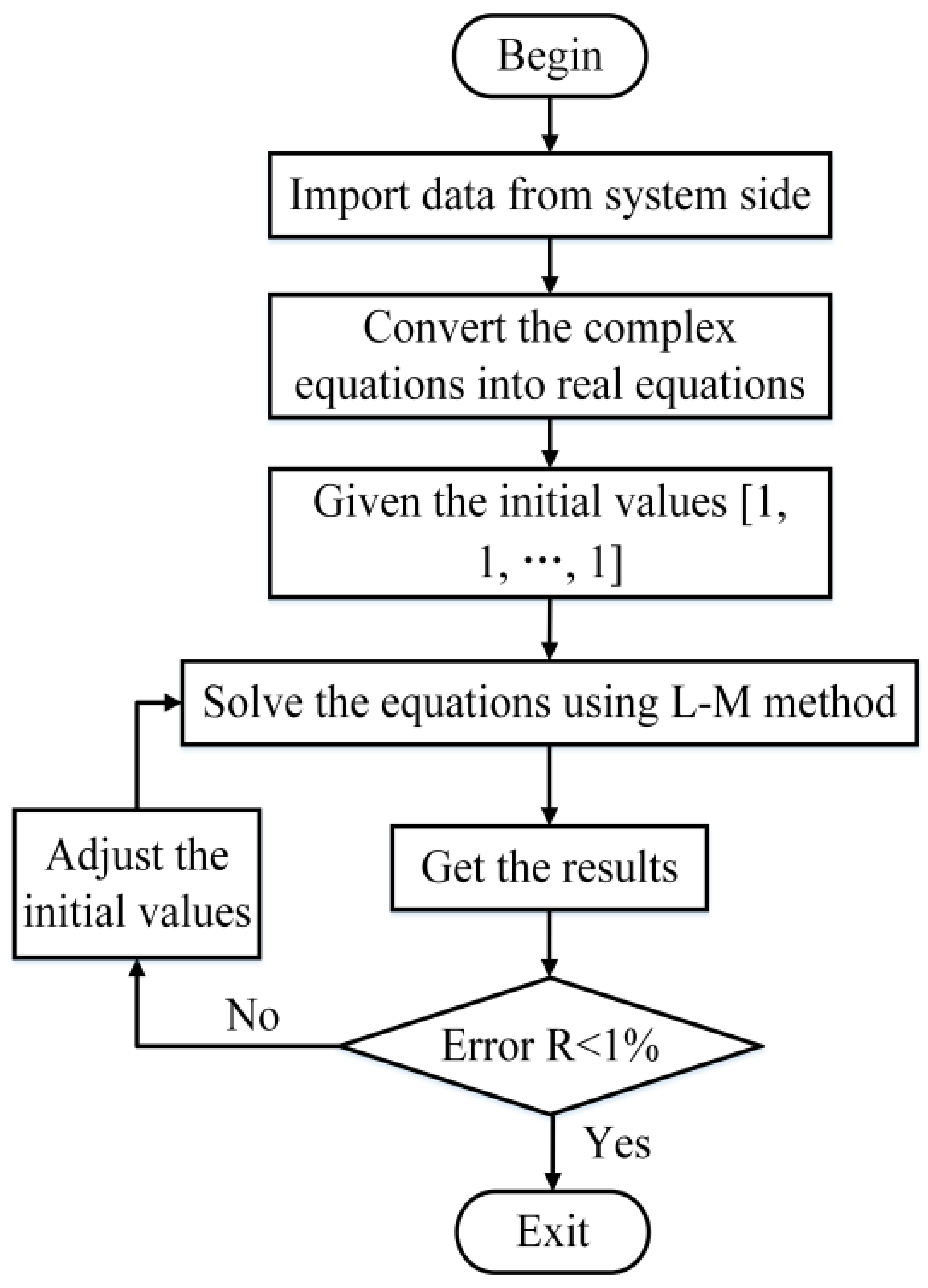
Define x = ( x 1 , , x 12 ) T , f ( x ) = [ f 1 ( x ) , , f 18 ( x ) ] T , and S ( x ) = f ( x ) T f ( x ) = f ( x ) 2 2 , then Equation (16) equals to f ( x ) = 0 , and the calculation to (36) equals to solve x* to make f ( x ) = 0 , while it also solves x* to make S ( x ) = min x R n S ( x ) and S(x*) = 0 [15]. The whole flow chart of employing the Levenberg–Marquardt algorithm to solve (38) is illustrated in Figure 2. And then the whole flow chart of the proposed fault location algorithm is shown in Figure 3.

4. Case Simulations

Case simulations are tested to prove the validity of the proposed method. The model is the same as that in Figure 1. The lengths of branches MP, NP, and KP are set to 50, 50, and 40 km, respectively. The electric potentials at terminals M, N, and K are 220 ∠ 0°, 220 ∠ 30°, and 220 ∠ 60°, respectively. A list of parameters for the simulation model (i.e., the power system and line sequence impedance) is displayed in Table 1.

4.1. The Impacts of Fault Distance

The fault distance from point P has increased from 5 km to 45 km in steps of 5 km. The fault resistance is 100 Ω. The fault localization results are listed in Table 2. It shows excellent fault location accuracy.

4.2. The Impacts of Fault Resistance

The fault resistance values are 5, 50, 100, 200, and 300, respectively, to test the error of the fault location algorithm. The results are shown in Table 3.
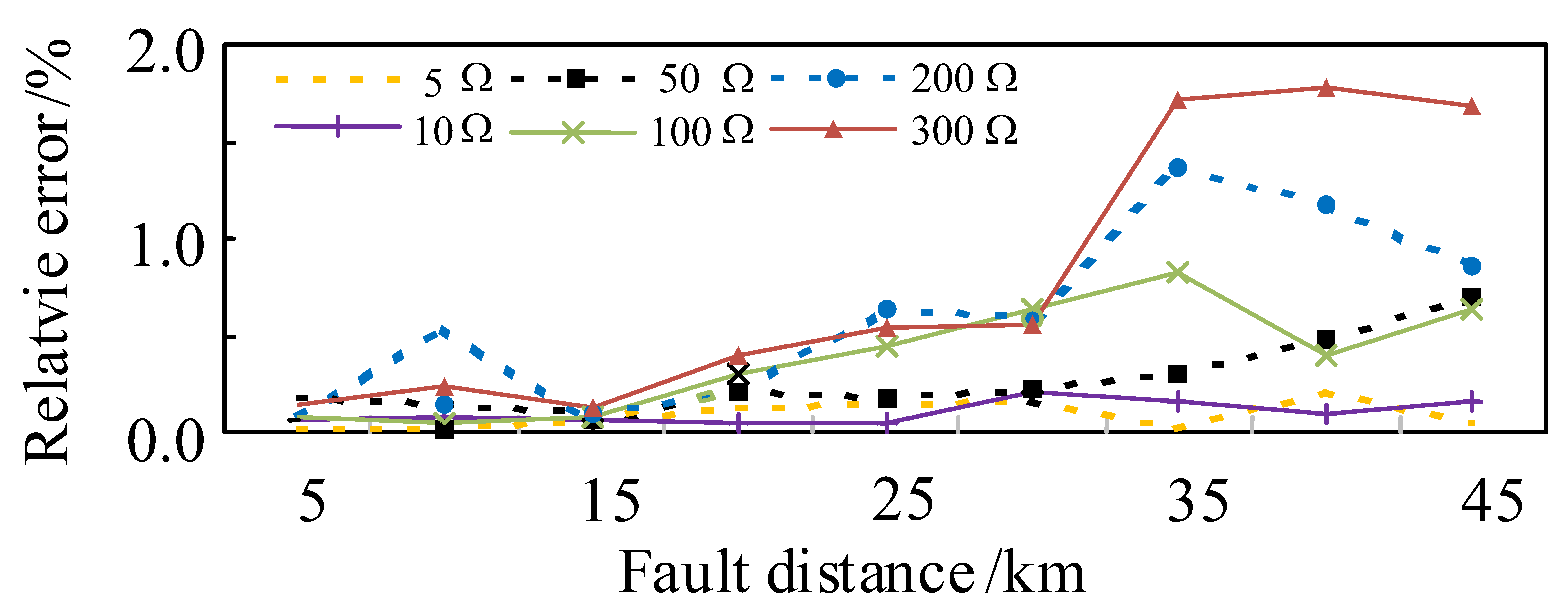
Figure 4 shows the fault localization error curves under different fault distances and fault resistances. The results indicate that the relative error of most fault location results is less than 1%. The maximum error is 1.78%, which occurs at fault distances of 40 km and high fault resistance of 300 Ω. The fault location error is affected by multiple parameters in the fault location equations, mainly due to the insignificant voltage drop between the fault point voltage and the branch point when the fault point is close to the N-side busbar and grounding through the large fault resistance. This can lead to the numerical solution algorithm of the fault location equations getting stuck in local optima and becoming unable to accurately identify the true fault point, resulting in significant fault location errors.

4.3. The Impacts of the Hypothetical Error of Equivalent Impedance of a Branch

In order to fully solve the fault location equations, it is assumed that the zero-sequence impedance of the branch is known, and therefore, the fault location error caused by the assumption error of the equivalent impedance of the branch should be evaluated.
In the simulated case of a fault resistance of 50 Ω, the exact zero sequence impedance in branch K is 29.09 ∠ 90°. The fault location results are shown in Table 4 by changing the size and angle of the assumed value of the K-terminal zero sequence impedance used in the algorithm calculation.
It shows that the hypothetical error of equivalent impedance of the branch can affect the fault location accuracy. In the case wherein the hypothetical amplitude varies by 30%, the maximum relative fault location error will reach 3.26%, and if the hypothetical angle varies by 20°, the maximum relative fault location error is 1.92%. Since the value of zero sequence equivalent system impedance is mainly decided by the grounding mode at the transformer neutral point, the grounding mode of the transformer usually keeps constant. So, the range of variation of zero sequence system impedance is limited, and then even if the hypothetical error of equivalent impedance of branch will decrease the fault location accuracy, the proposed method in the paper still can provide satisfactory applications in the field.
Through the above simulations, the following results can be obtained: The fault location algorithm for T-connected transmission lines proposed in the paper can achieve accurate fault location based solely on measuring voltage and current at one end. The essence of achieving this good fault location accuracy is to utilize the multiple stages of information before and after the tripping of the fault phase circuit breaker, construct a complete fault distance equation, and, thus, achieve accurate calculation of fault distance. Even in the most severe cases, the fault location error is not more than 3% in simulations, which can fully meet the application requirements of practical engineering.

5. Conclusions

In T-connection transmission lines, fault localization is a difficult problem because traditional fault localization requires synchronization and the communication of data from three terminals, and in practice, it is difficult to ensure good synchronization among them. A new single-ended fault location method has been proposed. It is based on the fact that the local topology of the T-connected power line in the healthy phases remains unchanged during the fault-clearing process. It utilizes the sequential current and voltage data changes generated by fault phase circuit breakers tripping sequentially from different terminals to describe the constant topology of the healthy phases as equations and calculates the accurate fault location after solving the equations. The Levenberg–Marquardt algorithm was used to calculate the fault distance and transition resistance, and the effectiveness of this method was verified through simulation. However, this paper focuses on traditional voltage source-dominated transmission systems, and in the future, this method can be further extended to wind power grid-connected transmission systems based on inverters.

Author Contributions

Conceptualization, B.W. and L.L.; methodology, B.W., H.Y. and Y.L. (Yuanyuan Lu); validation, Y.L. (Yang Liu) and W.L. All authors have read and agreed to the published version of the manuscript.

Funding

This research was funded by the science and technology project of State Grid Shandong Electric Power Company entitled “Research and application of enhancement technology for primary and secondary devices fused feeder automation supporting flexible operation of dual high active distribution networks” (52062622000T).

Data Availability Statement

The original contributions presented in the study are included in the article, further inquiries can be directed to the corresponding author.

Conflicts of Interest

Authors Lisheng Li, Haidong Yu, Yang Liu and Wenbin Liu were employed by the company State Grid Shandong Electric Power Research Institute. The remaining authors declare that the research was conducted in the absence of any commercial or financial relationships that could be construed as a potential conflict of interest.

References

  1. Guo, G.; Zha, K.; Zhang, J.; Wang, Z.; Zhang, F.; Cao, J. Grounding fault in series-connection-based offshore wind farms: Fault clearance. IEEE Trans. Power Electron. 2020, 35, 9357–9367. [Google Scholar] [CrossRef]
  2. Ajinkya, J.S.; Amod, C. Umarikar. Small-signal stability analysis of PV-based synchronverter including PV operating modes and DC-Link voltage controller. IEEE Trans. Ind. Electron. 2022, 69, 8028–8039. [Google Scholar]
  3. Naidu, O.D.; Pradhan, A.K. Precise Traveling Wave-Based Transmission Line Fault Location Method Using Single-Ended Data. IEEE Trans. Ind. Inform. 2021, 17, 5197–5207. [Google Scholar] [CrossRef]
  4. Lopes, G.N.; Menezes, T.S.; Gomes, D.P.S.; Vieira, J.C.M. High Impedance Fault Location Methods: Review and Harmonic Selection-Based Analysis. IEEE Open Access J. Power Energy 2023, 10, 438–449. [Google Scholar] [CrossRef]
  5. Terzija, V.; Preston, G.; Stanojević, V.; Elkalashy, N.I.; Popov, M. Synchronized measurements-based algorithm for short power line fault analysis. IEEE Trans. Smart Grid 2015, 6, 2639–2648. [Google Scholar] [CrossRef]
  6. Davoudi, M.; Sadeh, J.; Kamyab, E. Parameter-free fault location for power lines based on optimization. IET Gener. Transm. Distrib. 2015, 9, 1061–1068. [Google Scholar] [CrossRef]
  7. Yuan, B.; Wang, B.; Lu, Y.; Lu, L.; Liu, H.; Chen, C.; Wu, L. Error analysis of single-end fault location for single-line-to-ground fault in power line with wind farm connection. Power Syst. Prot. Control 2016, 44, 63–69. [Google Scholar]
  8. Jiang, J.; Chuang, C.; Wang, Y.; Hung, C.; Wang, J.; Lee, C.; Hsiao, Y. A hybrid framework for fault detection, classification, and location-part I: Concept, structure, and methodology. IEEE Trans. Power Deliv. 2011, 26, 1988–1998. [Google Scholar] [CrossRef]
  9. Wang, B.; Dong, X.; Lan, L.; Xu, F. Novel location algorithm for single-line-to-ground faults in power line with distributed parameters. IET Gener. Transm. Distrib. 2013, 7, 560–566. [Google Scholar] [CrossRef]
  10. Zhang, S.; Gao, H.; Song, Y. A new fault location algorithm for extra-high-voltage mixed lines based on phase characteristics of the hyperbolic tangent function. IEEE Trans. Power Deliv. 2016, 31, 1203–1212. [Google Scholar] [CrossRef]
  11. Ji, L.; Booth, C.; Dyśko, A.; Kawano, F.; Beaumont, P. Improved fault location through analysis of system parameters during autoreclose operations on power lines. IEEE Trans. Power Deliv. 2014, 29, 2430–2438. [Google Scholar] [CrossRef]
  12. Geng, J.; Wang, B.; Dong, X. A novel one-Terminal single-line-to-ground fault location algorithm in power line using post-single-phase-trip data. Trans. China Electrotech. Soc. 2015, 30, 184–193. [Google Scholar]
  13. Anderson, P.M. Power System Protection; Wiley-IEEE Press: Hoboken, NJ, USA, 1998. [Google Scholar]
  14. Hartley, H.O. The modified Gauss-Newton method for the fitting of non-linear regression functions by least squares. Technometrics 1961, 3, 269–280. [Google Scholar] [CrossRef]
  15. Moré, J.J. The Levenberg-Marquardt Algorithm: Implementation and Theory, Numerical Analysis; Springer: Berlin/Heidelberg, Germany, 1978; pp. 105–116. [Google Scholar]
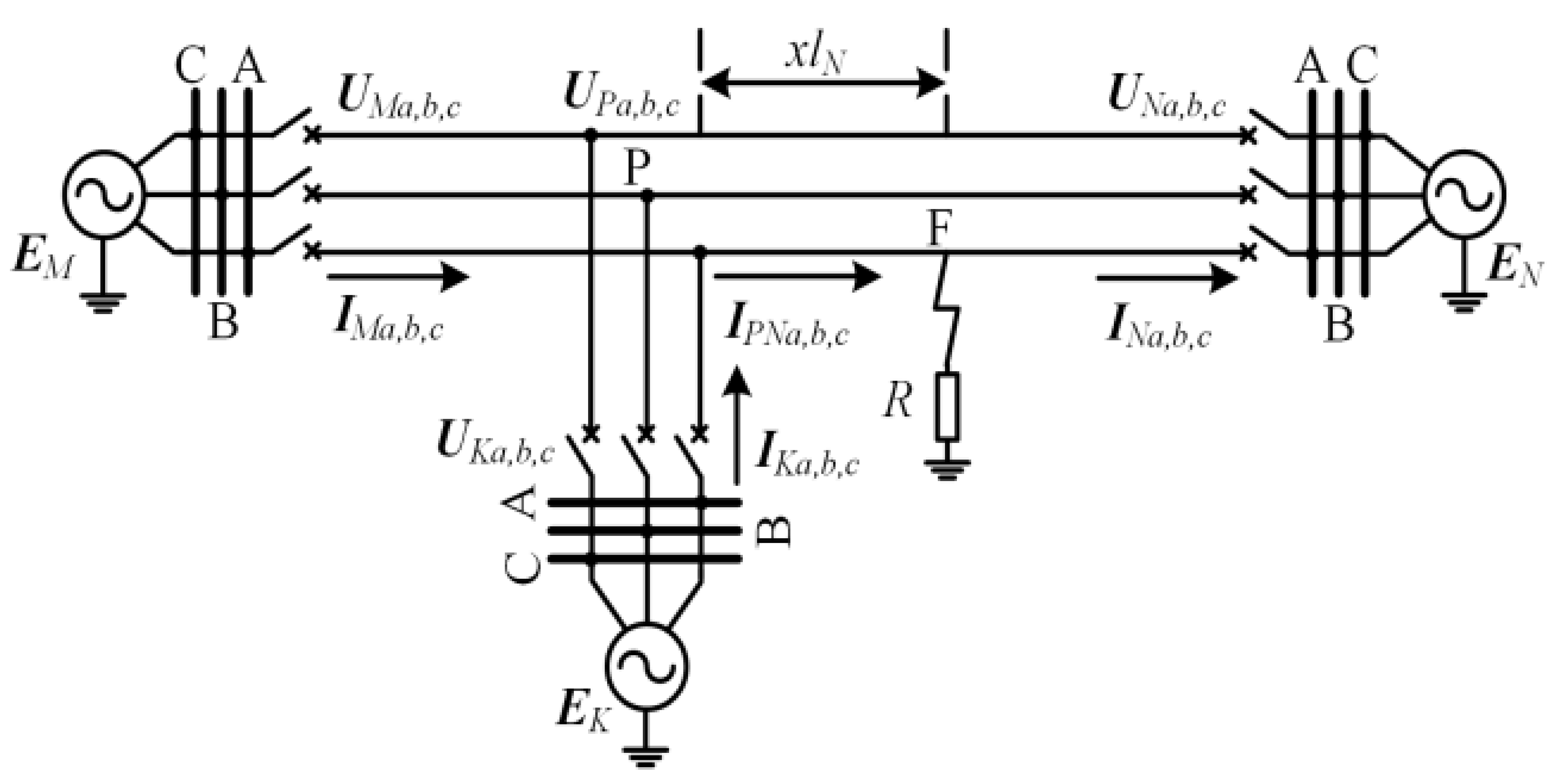
Figure 1. The topology structure of T-connected power lines.
Energies 17 02975 g001
Figure 2. Flow chart of employing the Levenberg–Marquardt algorithm to solve equations.
Energies 17 02975 g002
Figure 3. Flow chart of fault location method for T-connection power line.
Energies 17 02975 g003
Figure 4. The fault localization error curves under different fault distances and fault resistances.
Energies 17 02975 g004
Table 1. Parameters for simulation system.
SequenceLine
(ohm/km)
M Side System
(ohm)
N Side System
(ohm)
K Side System
(ohm)
Positive Seq.0.02 + j 0.2828.3 ∠ 90°32 ∠ 78.4°43.2 ∠ 88.6°
Zero Seq.0.172 + j 0.8426.3 ∠ 90°28.14 ∠ 86.7°29.09 ∠ 90°
Table 2. Fault location results under different fault distances.
Fault Distance (km)Calculated Distance (km)Absolute Error (km)Relative Error (%)Calculated R (ohm)
54.97−0.03−0.06100.03
1010.020.020.0499.99
1514.96−0.04−0.0899.99
2020.150.150.3099.99
2524.79−0.21−0.42100.06
3030.320.320.6499.92
3534.60−0.40−0.80100.13
4039.80−0.20−0.40100.07
4545.320.320.6499.90
Table 3. Fault location results under different fault resistances.
Grounding Resistance (ohm)Fault Distance (km)Calculated Distance (km)Absolute Error (km)Relative Error (%)
51010.270.270.54
2524.93−0.07−0.14
4039.90−0.10−0.20
501010.010.010.02
2524.92−0.08−0.16
4040.240.240.48
1001010.020.020.04
2524.79−0.21−0.42
4039.80−0.20−0.40
200109.93−0.07−0.14
2524.68−0.32−0.64
4040.590.591.18
3001010.120.120.24
2524.73−0.27−0.54
4040.890.891.78
Table 4. Fault location results under equivalent impedance estimation of branch with error.
Assumed Zero Sequence Impedance at K TerminalFault Distance (km)
51525303545
29.09 ∠ 90°4.9915.0324.9230.1134.8644.66
39.82 ∠ 90°5.2715.4925.5830.8835.7145.69
20.36 ∠ 90°4.7114.524.1129.1833.843.37
29.09 ∠ 80°5.1015.2125.1630.4035.1845.05
29.09 ∠ 70°5.2215.3925.4230.6835.4945.44
Disclaimer/Publisher’s Note: The statements, opinions and data contained in all publications are solely those of the individual author(s) and contributor(s) and not of MDPI and/or the editor(s). MDPI and/or the editor(s) disclaim responsibility for any injury to people or property resulting from any ideas, methods, instructions or products referred to in the content.