Article

Example of Using Particle Swarm Optimization Algorithm with Nelder–Mead Method for Flow Improvement in Axial Last Stage of Gas–Steam Turbine

by
Paweł Ziółkowski
1,*,
Łukasz Witanowski
2,
Stanisław Głuch
1,
Piotr Klonowicz
2,
Michel Feidt
3 and
Aimad Koulali
1
1
Institute of Energy, Faculty of Mechanical Engineering and Ship Technology, Gdańsk University of Technology, 80-233 Gdańsk, Poland
2
Institute of Fluid-Flow Machinery Polish Academy of Sciences, 80-231 Gdańsk, Poland
3
Laboratory of Energetics & Theoretical & Applied Mechanics (LEMTA), CNRS, Lorraine University, F-54000 Nancy, France
*
Author to whom correspondence should be addressed.
Energies 2024, 17(12), 2816; https://doi.org/10.3390/en17122816
Submission received: 15 March 2024 / Revised: 3 June 2024 / Accepted: 3 June 2024 / Published: 7 June 2024
(This article belongs to the Section I2: Energy and Combustion Science)

Abstract

:
This article focuses principally on the comparison baseline and the optimized flow efficiency of the final stage of an axial turbine operating on a gas–steam mixture by applying a hybrid Nelder–Mead and the particle swarm optimization method. Optimization algorithms are combined with CFD calculations to determine the flowpaths and thermodynamic parameters. The working fluid in this study is a mixture of steam and gas produced in a wet combustion chamber, therefore the new turbine type is currently undergoing theoretical research. The purpose of this work is to redesign and examine the last stage of the gas–steam turbine’s flow characteristics. Among the optimized variables, there are parameters characterizing the shape of the endwall contours within the rotor domain. The values of the maximized objective function, which is the isentropic efficiency of the turbine stage, are found from the 3D RANS computation of the flowpath geometry changing during the improvement scheme. The optimization process allows the stage efficiency to be increased by almost 4 percentage points. To achieve high-quality results, a mesh of over 20 million elements is used, where the percentage error in efficiency between the previous and current mesh sizes drops below 0.05%.

1. Introduction

Steam turbines are considered the backbone of power generation in many parts of the world, especially in Poland [1]. Their efficiency, therefore, has a direct impact on the overall performance of power plants and, consequently, on the cost and environmental footprint of electricity production. Recent studies have explored various strategies to optimize the efficiency of these turbines, focusing on aspects such as thermal integration [2], design parameters [3], and device modeling [4]. Steam turbines, often considered an ‘old technology’, continue to be an area of extensive research and development, targeting improvements in their efficiency, their operational flexibility [5], and their range of applicability [6]. These turbines are not just restricted to traditional power plant setups but are also being tailored to novel concepts of power plants, such as solar power plants [7], carbon capture [8,9,10], storage technologies [11], oxy-fuel technology [12,13], waste-to-energy plants [14,15], nuclear power systems [16], ORC [17,18], and electricity/hydrogen/synfuel polygeneration plants [19]. In this context, the role of simulation and optimization codes is pivotal, providing predictions on the effects of design/control improvements on the overall performance of the power plant. The design optimization of non-conventional steam cycles, such as integrated gas–steam combined cycles, presents more complex challenges due to the combinatorial nature of the heat exchanger network arrangement and specific working fluid, leading to a multitude of possible flowpath configurations [20,21,22]. The process of 3D optimization for a multi-stage turbine is an endeavor that demands significant time and computational resources [23]. Owing to this, when dealing with steam turbines, researchers often pay attention to the optimization of just the final stage of the turbine. The last stage has the highest power output of all stages. The stage analyzed in this paper has a 13.73 MW power output, which was determined during the 0D design [9].
The strategy of focused optimization represents a practical approach in computational engineering, demonstrating a balance between computational feasibility and the pursuit of performance enhancements in the complex realm of multi-stage turbine systems [24]. Sui et al. [25] undertook the multi-objective aerodynamic optimization of the last-stage blade in a 100 Hz industrial gas turbine. Aimed at maximizing the stage’s efficiency while ensuring mechanical integrity, the optimization strategy kept certain variables constant. Post-optimization, decreases in the peak Mach number, profile loss, and endwall loss were observed, improving the flow field and mechanical stress conditions of the blade. The optimized stage efficiency rose from 93.4% to 94.3% at the design point, with significant improvements in the blade strength. The study concluded by suggesting the design of fewer, longer chord blades for the final stage to enhance the efficiency and strength. Dolatabadi et al. [14] investigated non-equilibrium phenomena and the associated damage in power plants, specifically focusing on a 200 MW steam turbine. A modified profile for stationary cascade blades was proposed using computational fluid dynamics (CFD) to ensure cost-efficiency. The research employed a wet steam model to scrutinize the flow behavior between the turbine blades, taking into account phenomena such as sonication and non-equilibrium conditions. The model, based on the Eulerian–Eulerian approach, incorporated factors like turbulence from droplets, condensation shocks, and aerodynamics. After validation against experimental data, the model was applied to blade design, specifically the entrance edge. Based on criteria including the erosion rate, Mach number, entropy, exergy destruction, and mass and heat transfer, an economically optimized blade model was proposed. The modified blade exhibited a reduction in the erosion rate, entropy generation, and exergy destruction by 88%, 0.13%, and 7%, respectively. Moreover, the blade modification resulted in monthly maintenance cost savings of USD 456. The study underscores the economic and performance benefits of using optimally structured steam turbine blades to minimize the damage caused by non-equilibrium flow behavior.
The task of selecting an appropriate optimization algorithm is not simple, as it could fundamentally determine the success of the optimization process. In recent years, there has been a discernible upswing in the popularity of hybrid algorithms, attributable to their enhanced operational efficiency and reliability. Hybrid algorithms, combining the strengths of various individual algorithms, provide an effective means to solve complex scientific problems [26]. They enhance the computational accuracy and efficiency by balancing global and local searches, thereby avoiding premature convergence. However, their success largely depends on their careful configuration and adaptation to specific problem domains. Their adoption has improved the reliability and efficiency of the results in fields: optimization [27], data analysis [28], and machine learning [24].
Oxy-combustion in gas–steam turbines has primarily been developed with a focus on the overall power plant efficiency and CO2 capture capacity [8,12]. The absence of extensive analyses can be attributed to the technological challenges associated with practical implementation. At least three oxy-fuel combustion cycle solutions are well known in the literature: firstly, the semiclosed oxy-fuel combustion combined cycle (SCOC-CC) [29]; secondly, the Allam cycle [30]; and thirdly, the E-MATIANT cycle [31]. Both the Allam cycle and E-MATIANT cycle increase the SCOC-CC cycle efficiency by 5.6% and 11.5%, respectively. However, two solutions are possible in the Allam cycle, namely the introduction of a multi-flow regenerator and the incorporation of a supercritical carbon dioxide (S-CO2) Brayton cycle with recompression, which increase the efficiency by 3.5% and 0.2%, respectively [32].
In addition, advancements in various cooling techniques, such as the injection of water or steam into the combustion chamber, are making it increasingly feasible to realize combustion in a stoichiometric mixture of fuel and oxygen with water cooling [33]. This study presents the optimization of the final stage of the turbine in a Brayton double cycle employing an oxy-fuel combustion plant. The system in Figure 1 is characterized by three devices: a wet combustion chamber (WCC), a spray ejector condenser (SEC), and the high and low parts of a gas–steam turbine (HP + LP).
Figure 1 shows a basic scheme of the thermodynamic cycle of the gas–steam turbine with the last low-pressure twisted blades of the rotor and stator, where the following auxiliary devices are included: C—compressor, HE—heat exchanger, CHE—condensate cooler, S—separator, G—electrical generator, P—pump. Moreover, the division of the stator and rotor in the last stage is assumed in Figure 1. In the WCC, a working medium contains YH2O = 0.804 steam and YCO2 = 0.193 CO2, which is the product of the combustion. The specific data for the last stage of the turbine are shown in Table 1. Therefore, in the analyzed stage, there is novel medium, namely a mixture of CO2 and H2O. The working temperature is significantly higher than in the last stage of conventional steam. This is the first attempt to design such a stage for this type of medium. Additionally, CFD with optimization gives possibilities that were not available previously. The properties of the mixture influence the geometry. It is therefore necessary to investigate how they affect the geometry and hence the feasibility of the structure. This is valuable to examine whether parameters such as the blade length should be designed for one or two low-pressure cylinders (cf. Figure 1).
The primary objective of this research is to contrast the total-to-static efficiency of the turbine’s low-pressure part modeled using the conventional flow approach versus its post-optimization performance. The optimization procedure employs the hybrid Nelder–Mead particle swarm optimization (HNMPSO) and computational fluid dynamics (CFD) methods. These techniques allow for a marked increase in efficiency and the geometric enhancement of the turbine’s last stage. The findings underscore the potential of computational and optimization techniques in improving the turbine parameters.

2. Methodology

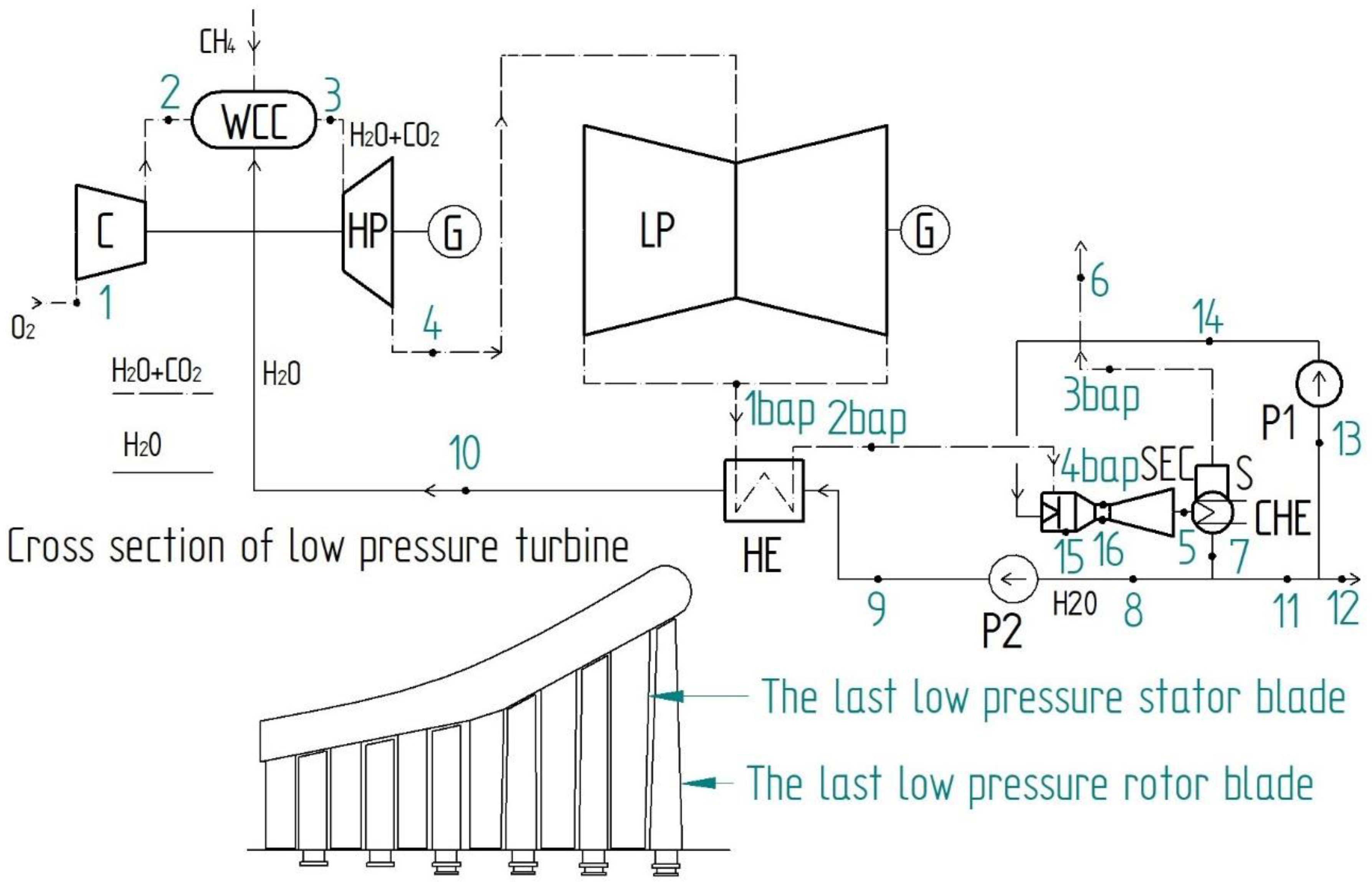
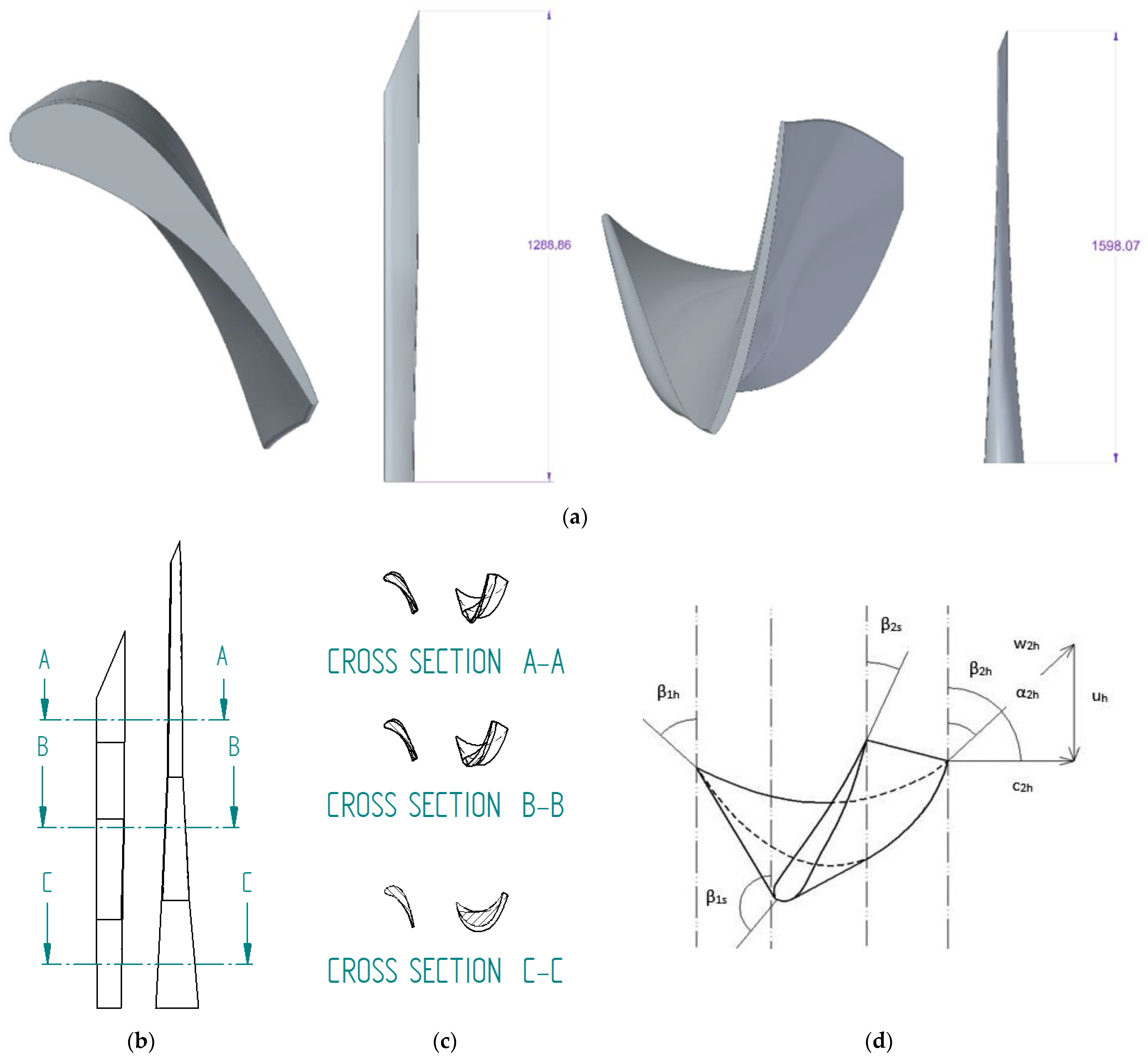
2.1. Twisted Stage Geometry Description

This article only refers to this type of system, where the influence of the long blades of the last turbine stage (shown in Figure 2) becomes apparent. As shown in Figure 2b, a characteristic feature is the change in stage reactivity with the height from the foot of the blade (hub); namely, at the bottom, it is an impulse. The higher it becomes, the more reactive it is. This result concerns the outcome of the design analyses presented in the authors’ previous paper [8,10]. However, it should be added that the initial blade design was presented in detail in [13]. Circumferential velocity u is dependent on the perimeter and thus the height of the blade. Velocity u significantly affects the velocity triangles. To meet the required velocity distribution across the turbine stages, most of the expansions have to take place at the rotor near the shroud area. Therefore, the angles and velocities presented in Table 2 have been implemented in a basic geometry.

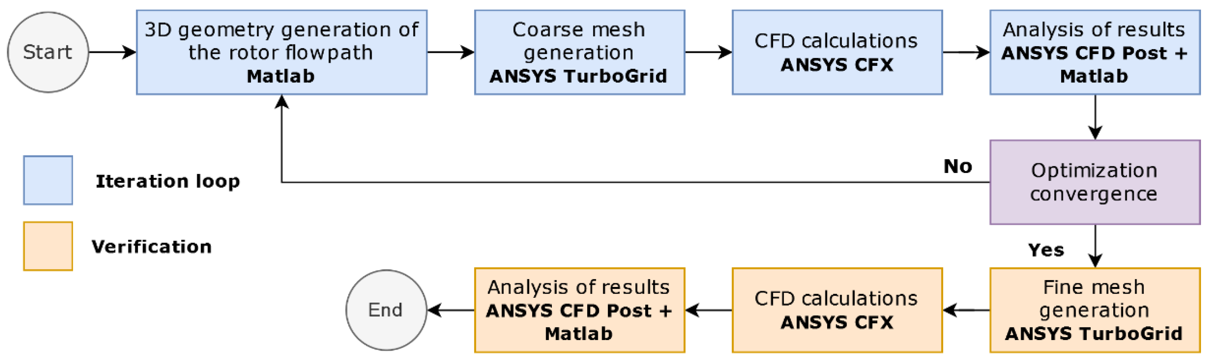
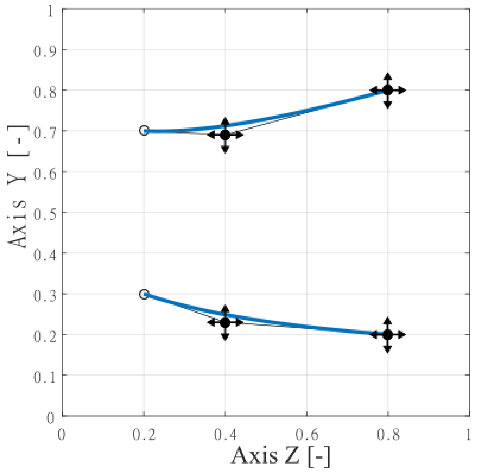
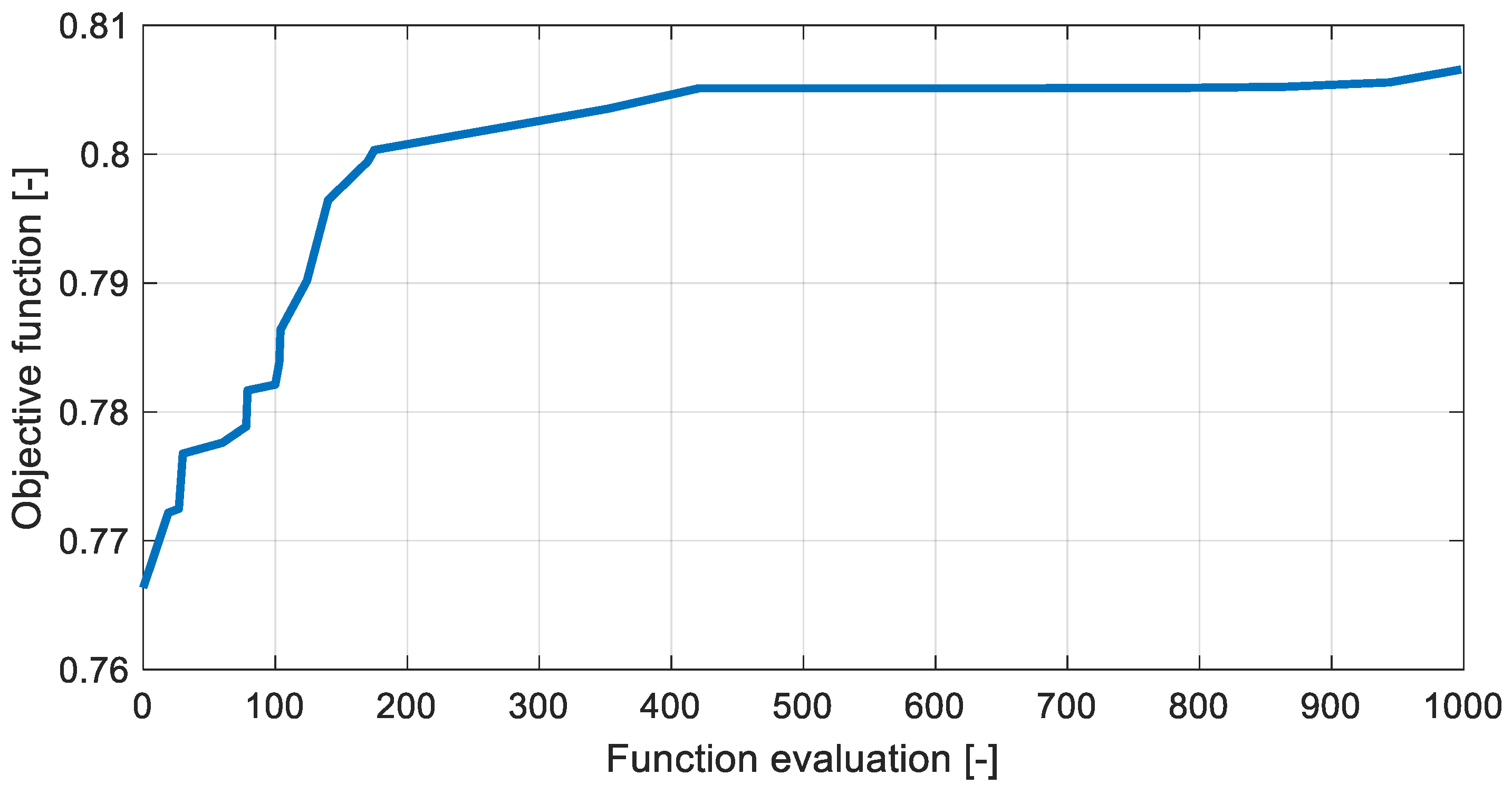
2.2. Optimization Framework

In design process the 27 stages of the HP and 6 stages in both directions of LP were generated. The kinematics and velocity vectors for all stages were designed. The rotor blade length for the last stage achieves 1587 mm (Figure 2). The law of velocity circumferential component variation of the working medium along the radius of the turbine blade was implemented. Furthermore, the design process uses a discrete way hence, the full 3D geometry of the blade can be developed. The circumferential velocity varies from 262 m/s near the blade hub to 771 m/s near the shroud.
To improve the performance of the present solution, CFD calculations using various optimization methods become necessary. In this study, a particle swarm optimization algorithm with the Nelder-Mead method for flow improvement in axial last stage of gas-steam cycle is used. This hybrid algorithm has proven its effectiveness in many engineering problems across different fields [34,35]. Therefore, it shows an initial 3D geometry of the stator and rotor blade designed basing on the free vortex law. The rotor blades are without tip clearance. The stage consists of 44 stator blades and 49 rotor blades. Almost 1 MW turbine stage has a process pressure drop from 16.6 kPa to 8 kPa. The Mach number at the stator exit equals 0.8. Additionally, the inlet temperature and rotor rotational speed is assumed as of 336.8 °C and 3000 rpm, respectively. The fluid mass flow rate reaches 91.15 kg/s. The last stage of the turbine is always a peculiar on [36], not only it is challenging from the material strength point of view, but also regarding the fluid flow.

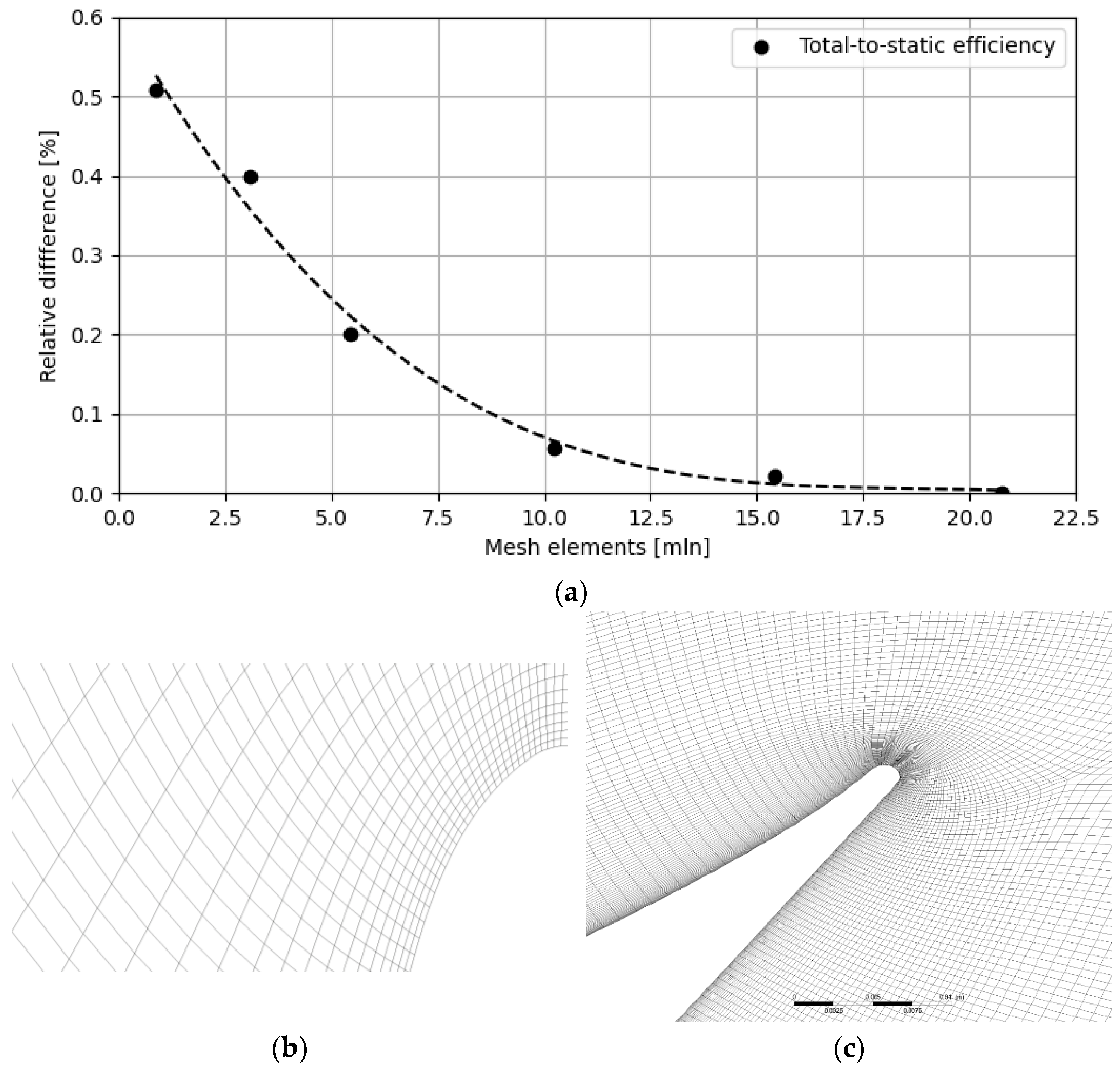
2.3. Computational Methodology

Steady-state Reynolds-averaged Navier–Stokes (RANS) calculations were executed utilizing the commercial code ANSYS CFX, paired with a second-order spatial discretization approach and an automatic timestep configuration. The selected set of boundary conditions comprised the total pressure, total temperature, and flow direction at the inlet; the average static pressure at the outlet; and the rotor domain’s rotational speed. To address the interface between stationary and rotating domains, the frozen rotor technique was assumed. It should be noted that the rotor blades were unshrouded. The working fluid’s characteristics were derived from the NIST Refprop Thermodynamic and Transport Properties database [37]. These models resolve a fundamental set of equations, specifically the mass, momentum, and energy balances for the fluid, in conjunction with the energy dissipation estimations.
The process of parametrizing the final 3D axial stage relied heavily on the adjustments made to the rotor meridional contour. The concept of endwall contouring is pursued in LP turbines, employing divergent contours to ensure a smooth flow at the endwalls and to instigate the streamline curvature that attenuates the downstream flow parameter gradients after the stator. This paper delineates the geometry of the meridional contours using two B-spline curves (third-order curves). The optimization parameters numbered eight: four for the lower endwall and four for the upper endwall. Each parameter was allowed to oscillate within a predefined range. As a consequence of modifying the meridional contours of the flowpath, the rotor blade’s height experienced changes.
To acquire a new shape, the method of linear extrapolation (with fixed parameters) was employed, facilitating the lengthening or shortening of the rotor blade. The introduced collaborative parallel algorithm is a composite of particle swarm optimization and the Nelder–Mead method, termed HNMPSO. In this method, the algorithm initiates with a randomly generated initial population. The entire population is sorted based on their fitness (value of the objective function). The optimal solutions are inputted into the deterministic algorithm to enhance the rank solution. The suboptimal solutions are diverted to the PSO method. The subsequent stage involves the standard procedure for the particle swarm optimization algorithm. In summary, the architecture of this hybrid algorithm circumvents stagnation and enables the potential construction of a simplex, encompassing several locally distinct minima. The comprehensive optimization procedure encompasses two stages—iteration and verification (Figure 3). Every aspect of the iteration loop is overseen by a script developed in the Matlab R2021a environment. The geometry of the optimized stage is formulated within this Matlab script. An automatic grid was established using the ANSYS TurboGrid 2021 R1 software.
The performance of the turbine stage is affected greatly when the assumption of a uniform channel height across the radius is disregarded [38,39]. The flow conditions vary with the radius of the last stage division, and, to enhance the efficiency of the turbine, the blade shape needs to be altered to adapt to these changes [19]. This is achieved by altering the inlet (α) and outlet (β) angles to match the fluctuating circumferential speed u. The process of adjusting the blade shape is referred to as twisting and is performed using the free vortex method, as described in detail in Reference [40]. In addition, the work will also refer to Professor Szewalski’s proposal [41,42,43] in the future.
Typically, the law for the distribution of the circumferential component of the fluid velocity in the radial direction, known as the law of coiling of the second blade, is best represented in a discrete form, which can differ for the inlet and outlet of the vane channel. In engineering practice, it is desired to have the lowest possible circumferential velocity component at the outlet to prevent an unnecessary increase in the dissipation of kinetic energy, which would decrease the efficiency [40]. The free vortex method is used to meet this requirement. The stage was divided into n = 15 sections, with a reaction ratio (ρ) of 0.1 at the hub to prevent ventilation work during partial loads.
l s = l s n ;   l r = l r n
n = 15 sections is the reason for the compromise because it ensures the creation of sufficient blade shape information and does not require significant time to create the first blade geometry, which is the subject of optimization. The length of the blades of the stator and rotor is the following: l s = 1289 mm and l r = 1587 mm, respectively. It is equally important to determine the inflow angle α1 in subsequent sections by using the relationship
tan α 1 h = α 1 m · π / 180 r h / r m ;   tan α 1 = r 2 r h · tan α 1 h
where r m —the medium radius, α 1 m —the medium angle of the inlet, α 1 h —the angle of the inlet at the hub, r 2 —the radius of the rotor for a given section, r h —the radius at the hub (blade foot of the rotor). The reactivity of the stage is determined based on the formula from Professor Perycz’s book [40]:
ρ = 1 ( 1 ρ h ) · ( r h r 1 ) k
where ρ h = 0.1 is the reactivity at the hub assumed as the initial one, r 1 is the the radius of the stage in a given section of the discernment, and k = 2 cos α 1 is the coefficient at the correction of reactivity. Based on the continuity equation, we determine the mass flow rate on particular sections:
m ˙ = μ 1 · c 1 s · A 1 · sin α 1 v 1 s
where A 1 = 2 · π · r 2 is the surface area of the given section, μ 1 is the coefficient, c 1 s is the absolute speed, and v 1 s is the relative speed. The calculation procedure also determines the angle β and the speed components for the individual speed triangles, as well as the blade losses for subsequent sections, the power, and the efficiency.
The calculation is performed iteratively and the comparison parameter is the mass flow, ensuring that the sum of the contributions ( m ˙ ) from each section of the stage equals m ˙ = 91.15 kg/s. Due to very large changes in the value of the circumferential velocity (u), there are large changes in the reactivity, angles, and velocity along the radius. The circumferential speed ranges from 262 m/s to 771 m/s, and the sound velocity in this area of the pair fluctuates around 440 m/s. It is important to note that, near the hub, the blade experiences a high impulse at the foot and a very high reaction ratio at the apex. The minimum reaction ratio (ρ) of 0.1 is located at the hub and should not drop below 0.1, to prevent negative values of the degree of reaction at a partial power loss. The reaction ratio near the shroud is as high as 0.89.
CFD resolves a set of basic equations, namely mass, momentum, and energy balance equations, for the fluid and energy dissipation equations. This set of basic equations, namely mass ( ρ ), momentum ( ρ v ), and energy ( ρ e ), can be written as follows:
t ρ + d i v ρ v = 0
t ρ v + d i v ρ v v + p I = d i v τ c + ρ b
t ρ e + d i v ρ e v + p v = d i v τ c v + q f l u i d C + ρ b v
where: ρ = ρ ( x , t ) defines fluid density, which generally depends on time t and location x ; v = v i e i represents fluid velocity; p is pressure, b gives gravity. Tensor connected with stress includes: unity tensor for reversible processes I = δ i j e i e j and the viscous, turbulent, and diffusive flux of momentum for irreversibility as follows τ c = τ + R + D . In energy balance crucial components are: e = u + v 2 2 as the sum of internal and kinetic energy, next q f l u i d C = q + q + + q p h + as total heat flux in the fluid. The influence of the turbulent transport of fluid momentum and heat should possess the set of additional equations governing the evolution of turbulent primary parameters, namely: turbulent kinetic energy k and turbulent dissipation energy ω . The turbulence model employed in this paper is Menter’s k ω SST, which can be written as follows [39,40]:
t ρ k + d i v ρ k v = d i v J k + S k
t ρ ω + d i v ρ ω v = d i v J ω + S ω
where: J k , J ω represents diffusive flux of k and diffusive flux of ω with sources S k , S ω , respectively to Equations (8) and (9) [9,44]. For each finite volume of the computational grid, seven equations are solved. Namely, five balance equations and two evolution equations have been described in publications [45]. The turbulent viscosity in (8) and (9) is computed by combining k and ω as follows [46]:
μ t = α ρ k ω
For low fluid velocities (laminar–turbulent transitions), the coefficient α damps the turbulent viscosity, causing a low Re number correction.
The parameterization of the last 3D axial stage was based on changing the rotor meridional contour. The idea of endwall contouring is pursued in LP turbines with diverging contours to ensure a smooth flow at the endwalls and to induce a streamline curvature that reduces the gradients of the flow parameters downstream of the stator [44]. In this paper, 3th order curves describe the geometry of meridional contours by two B-splines. The 4 parameters for the lower endwall and 4 for the upper endwall were implemented for the optimization. Figure 4 demonstrates that each parameter varies in a prescribed range. Due to modifying the meridional contours of the flowpath, the height of the rotor blade changes. By reaching a new shape, the linear extrapolation is used, which allows the rotor blade to be shortened or lengthened, respectively.
The isentropic total-to-static efficiency is selected as the objective function for the optimization of the last turbine stage, which can be described as follows:
η t s = h 0 T h 2 T h 0 T h 2 s
With this definition, the exit kinetic energy losses are included in the objective function formula [45]. However, the isentropic total-to-total efficiency is determined as follows:
η t t = h 0 T h 2 T h 0 T h 2 s c 2 2 2
Equation (12) is also helpful in optimization.

2.4. Method Validation

To perform simulation properly the discretization of the analyzed domain must be gained correctly with the inclusion of crucial elements. Thus, the hexahedral mesh has been selected, as one that provides excellent accuracy and a relatively low element count. Figure 5a illustrates the relative maximum difference values of total-to-static efficiency for the analyzed computational meshes, compared to the reference values obtained from the mesh with the largest grid cell count. Differences in efficiency below 0.1% are already visible in a mesh consisting of about 10 million elements. Further increases in mesh size result in a slight decrease in the efficiency obtained. To achieve high-quality results, a mesh of over 20 million elements was used, where the percentage error in efficiency between the previous and current mesh sizes dropped below 0.05%.
In the iteration phase, to do calculations in a reasonable time, a reference mesh, presented in Figure 5b, consisting of 1 mln hexahedral elements are applied. Mesh limits are established on the maximum face angle (165°), minimum face angle (15°), connectivity number (12), maximum and minimum volume ratio (10 and 0) and maximum edge length ratio (1000) [46]. In the verification phase, showed in Figure 5c, the optimal geometry is simulated on a fine grid of 20 mln nodes per stage.
Another aspect of the calculation methodology is the introduction of hybrid algorithms. Hybridization links two or more algorithms which run together and complement each other to give a profitable synergy from their integration [47]. Hybridization purposes to join the advantages of each algorithm, whilst reducing the disadvantages [48]. In hybrids, one algorithm may be incorporated as a sub-algorithm to locate the optimal parameters for another program. Alternatively, different components of the algorithm like the mutation crossover are applied to enhance another algorithm in the hybrid structure. The hybrid algorithms can be segregated as follows: collaborative hybrids and integrative hybrids. Depending on the combination of the running algorithm, the weight of participating in the collaborative hybrids can be grouped: multi-stage, sequential, and parallel. Others Genetic Algorithms [49] which work well with CFD methods are applied simultaneously.
The proposed collaborative parallel algorithm is a combination of particle swarm optimization [50] and the Nelder–Mead method [51], called HNMPSO [52,53,54,55].
Nelder–Mead Method: This is a simplex-based method that does not require the calculation of derivatives, making it suitable for optimizing non-smooth functions. The method manipulates a simplex (a geometric figure formed by N + 1 vertices in N dimensions) to explore the search space [56]. Key operations include the reflection, expansion, contraction, and shrinkage of the simplex based on the function values at its vertices. It iteratively adjusts the simplex and moves towards the minimum or maximum through local search operations. The method is deterministic in its adjustment steps and relies heavily on the geometry of the simplex.
Particle swarm optimization (PSO): PSO is a population-based stochastic optimization technique inspired by the social behavior of birds or fish. It involves a number of ‘particles’ that move through the solution space, guided both by their individual best-known positions and the overall best-known positions within the swarm, adjusting their velocities dynamically based on these insights. PSO explores the search space through a combination of random and collective behavior, making it inherently stochastic [57,58]. It is more likely to avoid being trapped in local optima compared to purely deterministic methods due to its global search capabilities, enabled by the swarm behavior.
In the HNMPSO method, the algorithm starts with the random generation of the initial population [52]. The entire population is sorted according to their fitness (the value of the objective function). The best solutions (N + 1) are fed into the deterministic algorithm to improve the (N + 1)th solution in the rank (point 6). The worst solutions (2N) are moved to the PSO method. The next step is the standard procedure for the particle swarm optimization algorithm (points 7–21). To sum up, the structure of this hybrid algorithm enables the avoidance of stagnation and the possibility of constructing a simplex consisting of several local minima that are significantly distant from each other.
Therefore, it is important to highlight the versatile application of optimization methods through turbines [44,45], energy pumps [59,60], and such pumps with blood flow [49].
The HNMPSO approach to optimization can significantly reduce the secondary flow losses as well as boundary-layer, separation, and exit energy losses and, as a consequence, improve the flow efficiency of turbine stages. Elements of the previous paragraphs were previously presented in [8,9,10].
In this work, the CFD calculation methodology follows the same published approach in our previous works [61,62]. Additionally, as mentioned earlier, mesh testing was conducted to ensure the accuracy of the results. Internal validation can also be drawn from the logical magnitudes of variables such as velocity, pressure, and Mach number, which align with the expected ranges for the engineering processes related to this problem. The CFD approach was complemented by the HNMPSO algorithm, as previously indicated. Its validation includes tests for the convergence of the objective function, as illustrated in Figure 6. Therefore, the optimization was executed using hybrid algorithm, a combination of a Nelder-Mead Method with Particle Swarm Optimization called HNMPSO with more than 1000 function evaluation. Figure 6 shows that the total-to-static efficiency of the low-pressure last stage turbine was radically improved.

3. Results and Discussion

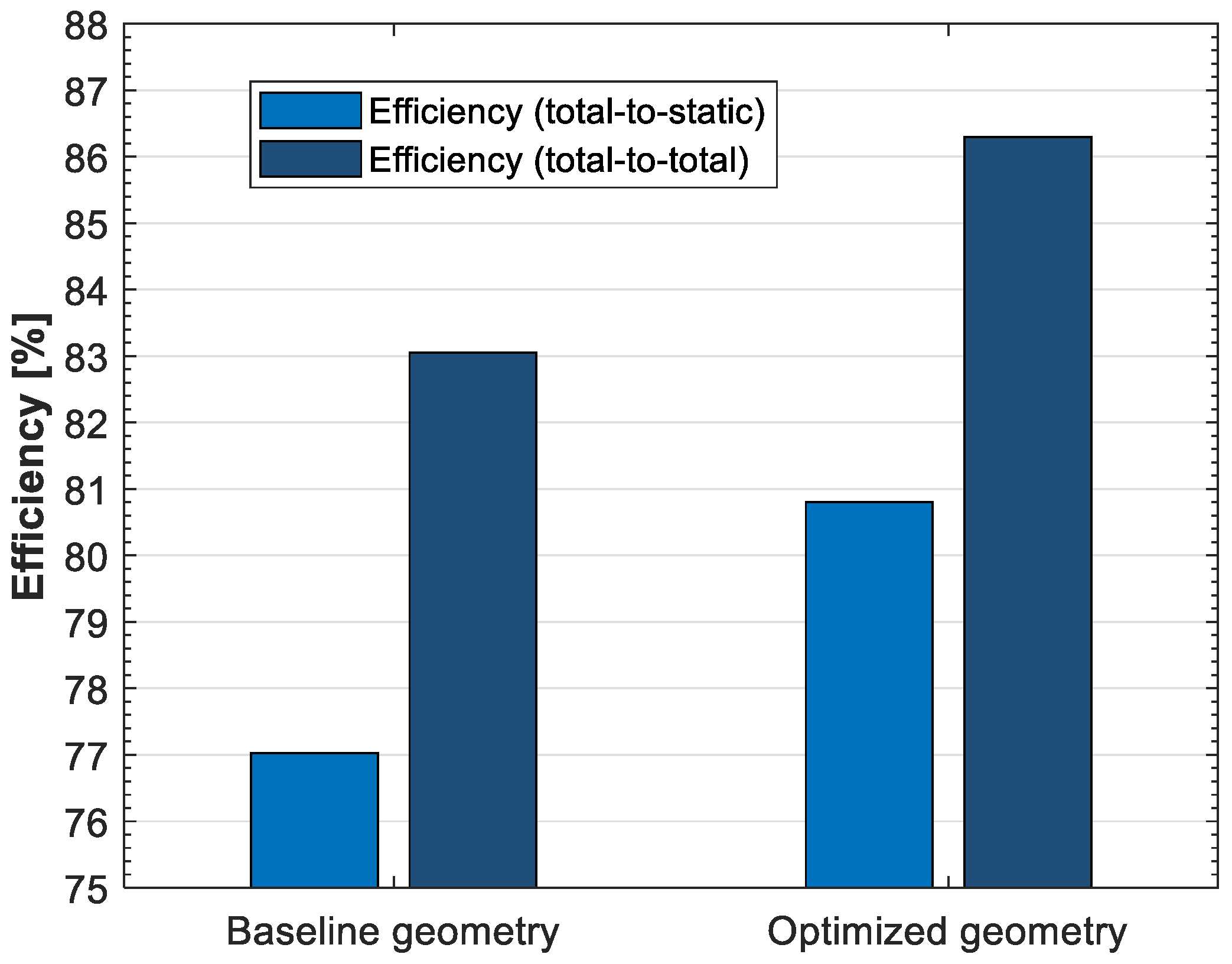
3.1. Comparison of Total-to-Static and Total-to-Total Efficiency

Figure 6 presents the final values of the efficiency. Nevertheless, Figure 7 shows the comparison of the total-to-static and total-to-total efficiency of the stage with respect to Equations (11) and (12). The outlet loss (or exit velocity loss) is connected with the unused kinetic energy of the fluid. It is defined as Δ i o u t = 1 2 c 2 2 , where c 2 is the turbine’s exit velocity. In particular, the areas of the rotor fluid achieved a higher velocity because of the more optimal flow distribution, but, as a result of the optimization, there was a reduction in the average velocity at the stage exit. Thus, the outlet loss was reduced by 5.88 percent. The static entropy, which represents losses, is presented in Figure 8.

3.2. Comparison of Geometry

The geometric changes between the baseline and optimized turbine stage are illustrated in Figure 9. As a result of the changing endwall contours, the flowpath exit area from the rotor passage was increased in the optimized design. The optimization algorithm plays a crucial role in the design process of turbine flow channels by determining the optimal geometric parameters that can enhance the turbine’s performance. This algorithm systematically adjusts various geometric characteristics to maximize the efficiency and minimize energy losses. Once the optimization algorithm identifies a promising set of geometric configurations, these configurations are then translated into detailed geometrical models of the turbine. These models serve as inputs for computational fluid dynamics (CFD) simulations, specifically conducted in sophisticated software like ANSYS CFX 2021 R1. The interplay between the optimization algorithm and CFD calculations is iterative. The initial results from the CFD simulations can be fed back into the optimization algorithm, prompting further adjustments to the geometric parameters to refine the design. This iterative process continues until the optimization converges on a design that meets the desired performance specifications, effectively balancing the efficiency, durability, and cost. Finally, the end of the lower endwall moved from 820 mm to about 770 mm. The upper endwall was changed significantly; the exit radius increased to 3000 mm. All changes and optimization boundaries are presented in [10]. Thus, this change in channel is more optimal from the point of view of the flow distribution, but the rotor blade would have to withstand higher centrifugal forces. Because of this, the blade should be checked in the next iteration of the stage design, which is the mechanical strength finite element simulation. Such analyses, along with stress optimization, are possible whether for pumps [63] or turbines [64,65].

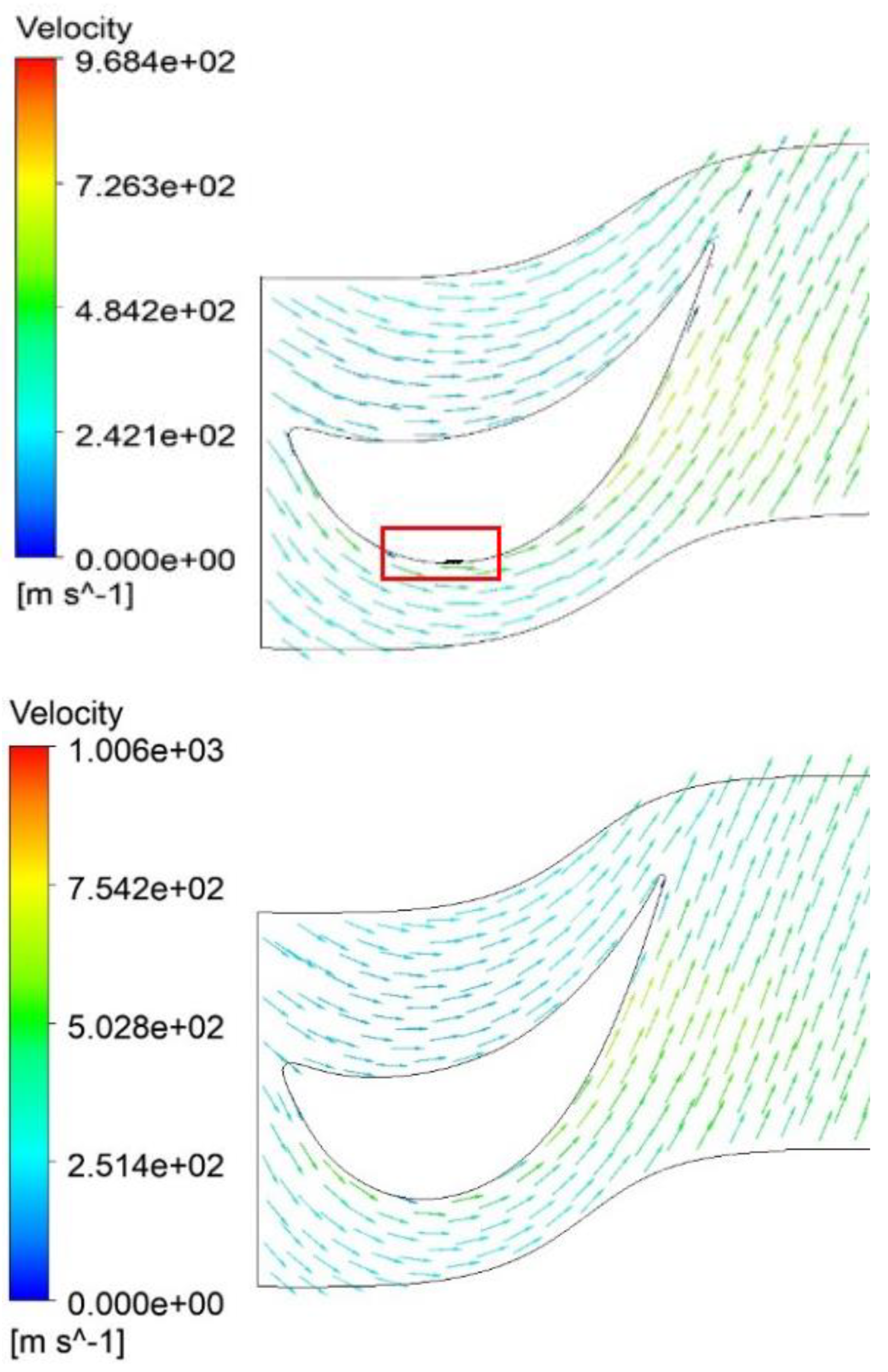
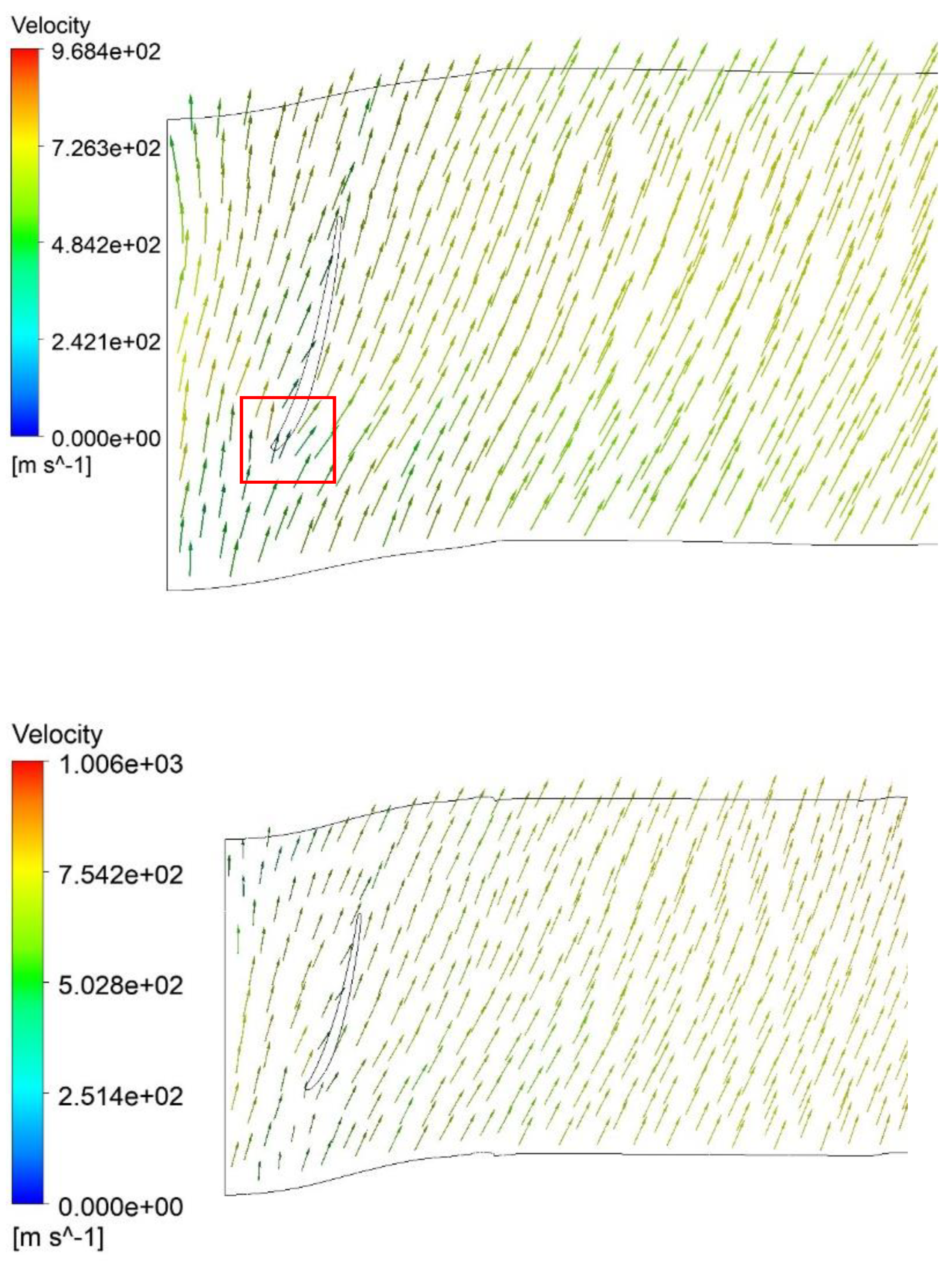
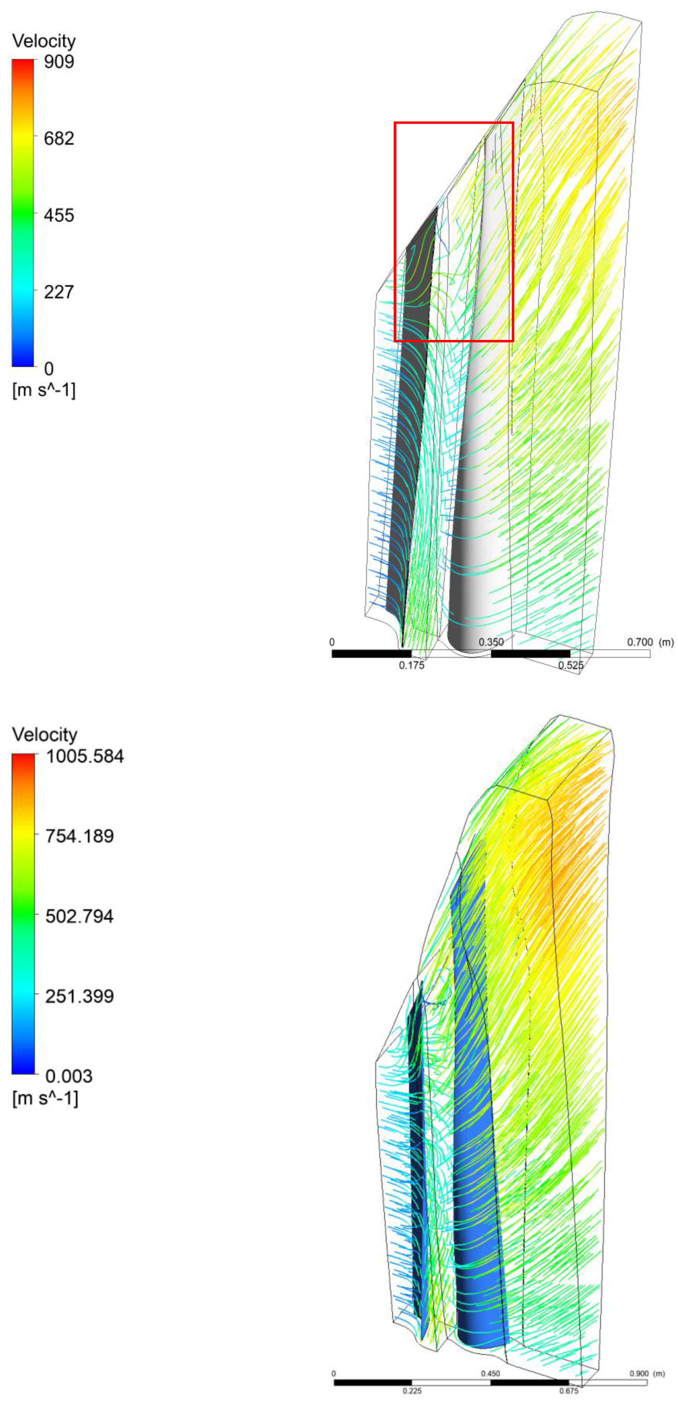
3.3. Comparison of Velocity

The comparison of the velocity vectors is illustrated in Figure 10, Figure 11 and Figure 12. Due to the changing meridional contours, the velocity vectors were varied. It should be noted that the profile loss at the hub was reduced in the optimized geometry. Moreover, the loss distribution on the shroud was marginally lower than for the original geometry.
The velocity vectors at the mid-span were also slightly improved (Figure 11), even though the area where the shape optimization took place was at the hub and the turbine’s inner casting (shroud)—see Figure 12. The area of flow separation at the mid-span was significantly reduced. The higher area of the blade was under the correct pressure and could generate momentum. The reason that the flow separation was still present after the optimization process was that the blade shape itself was not changed during the simulations. The area of flow separation was also reduced at the shroud. Figure 13, Figure 14 and Figure 15 present the Mach number. The Mach number and velocity achieved higher local maxima, which led to increased pressure differences at both sides of the blade, which contributed to the increase in the stage efficiency. The average velocity at the outlet was lower after optimization. The streamlines in the baseline design (above) and optimized design (below) are included in Figure 16. This figure confirms the improved flow with the decreasing vortex structures. Based on the presented results for the velocity vectors, Mach numbers, and streamlines, it should be concluded that the flow is clearly turbulent. As indicated in the Methodology, a laminar model is unnecessary and focusing on turbulence models is more appropriate to accurately simulate such flow dynamics. The Reynolds number ranges from 16,544.4 at the hub to 39,944.4 at the shroud. The characteristic length was assumed as the distance between the blades that gave the lowest value of the Reynolds number. Therefore, all calculated values are well beyond the pipe transition value of 2300 and there is a turbulent flow.
By modifying the meridional contours within the turbine, the development and extent of the secondary flows are effectively reduced. This modification impacts the overall flow dynamics by minimizing the flow losses that typically occur due to turbulent interactions and inefficiencies in the fluid movement. Studies have shown a decreased interaction between the secondary flows and the boundary layers on the suction sides of the blades in channels with optimized contours (cf. Figure 13, Figure 14 and Figure 15). This reduced interaction helps in maintaining a more streamlined flow, thereby enhancing the aerodynamic efficiency of the turbine. The improvements in efficiency stemming from these modifications also result from the more favorable outlet angle (cf. Figure 10, Figure 11 and Figure 12 for the optimized design (below)). A well-optimized outlet angle ensures that the fluid exits the turbine in a direction that maximizes the extraction of kinetic energy and minimizes the backflow and vortex formation at the blade tips, which are common sources of energy losses.

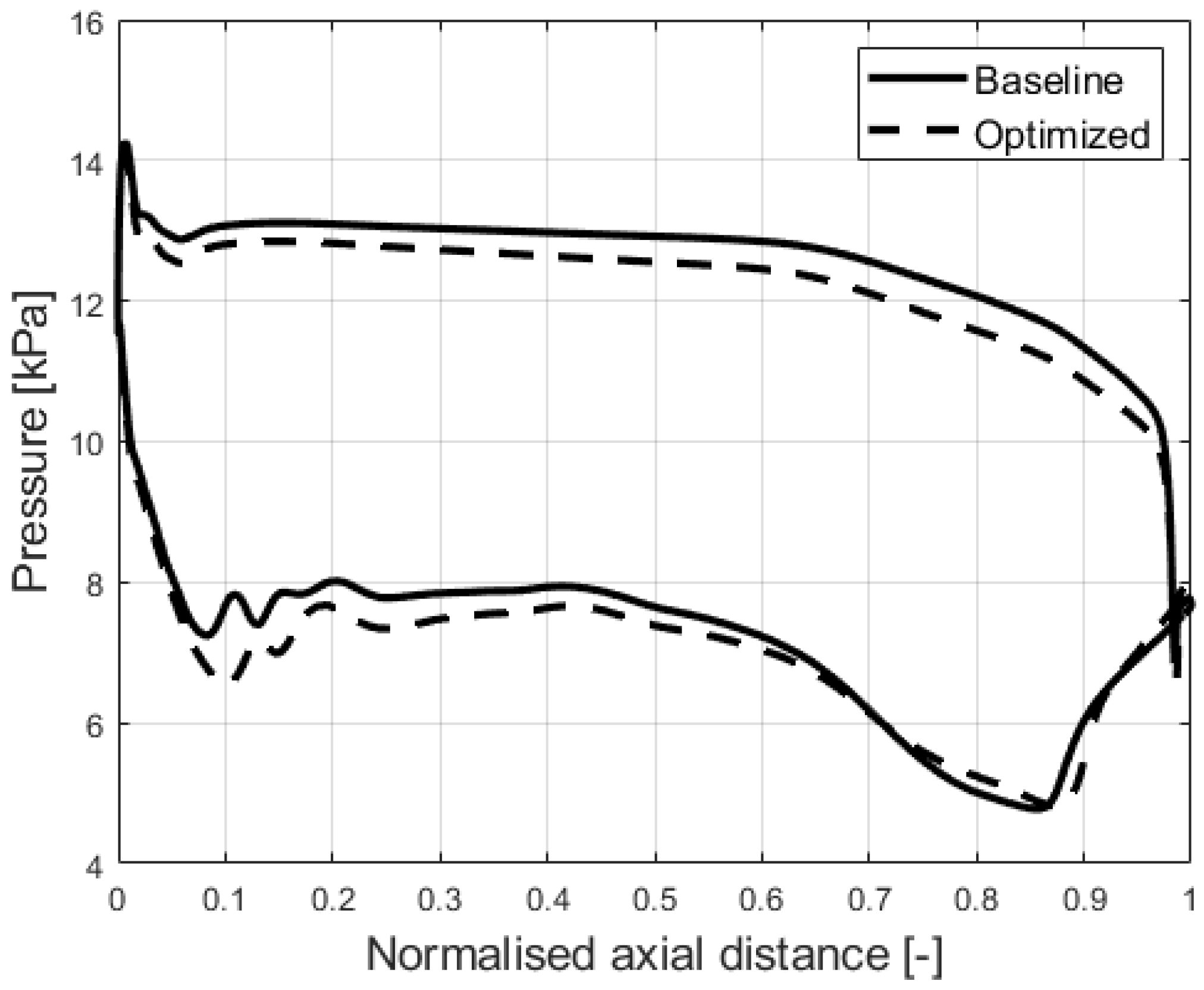
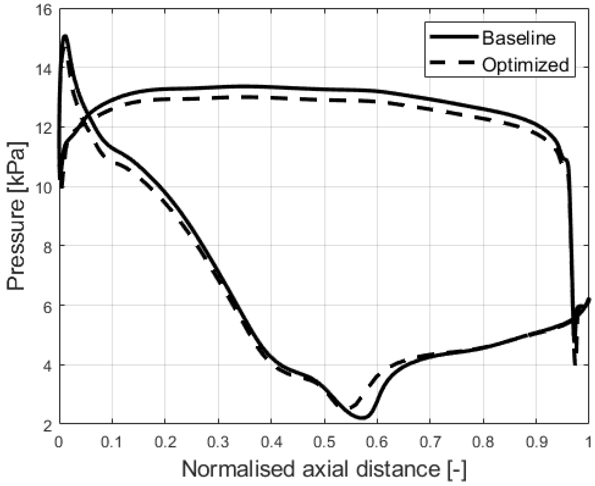
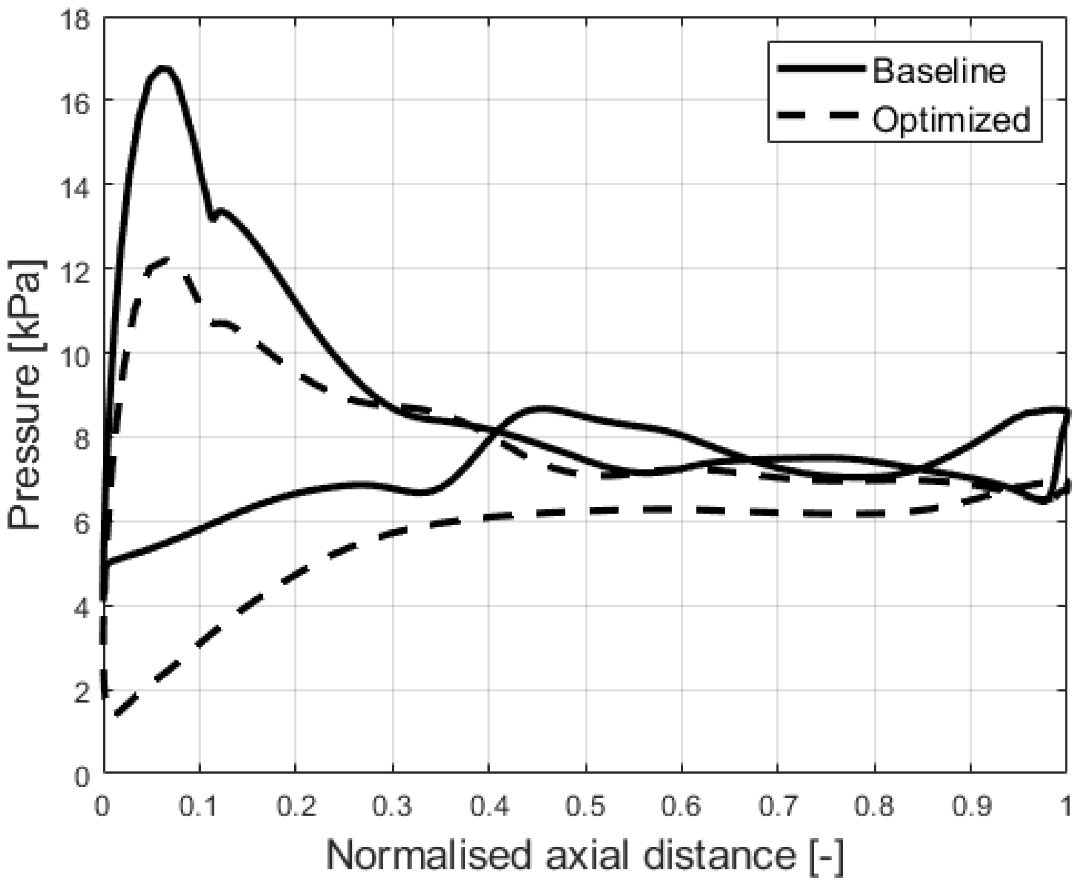
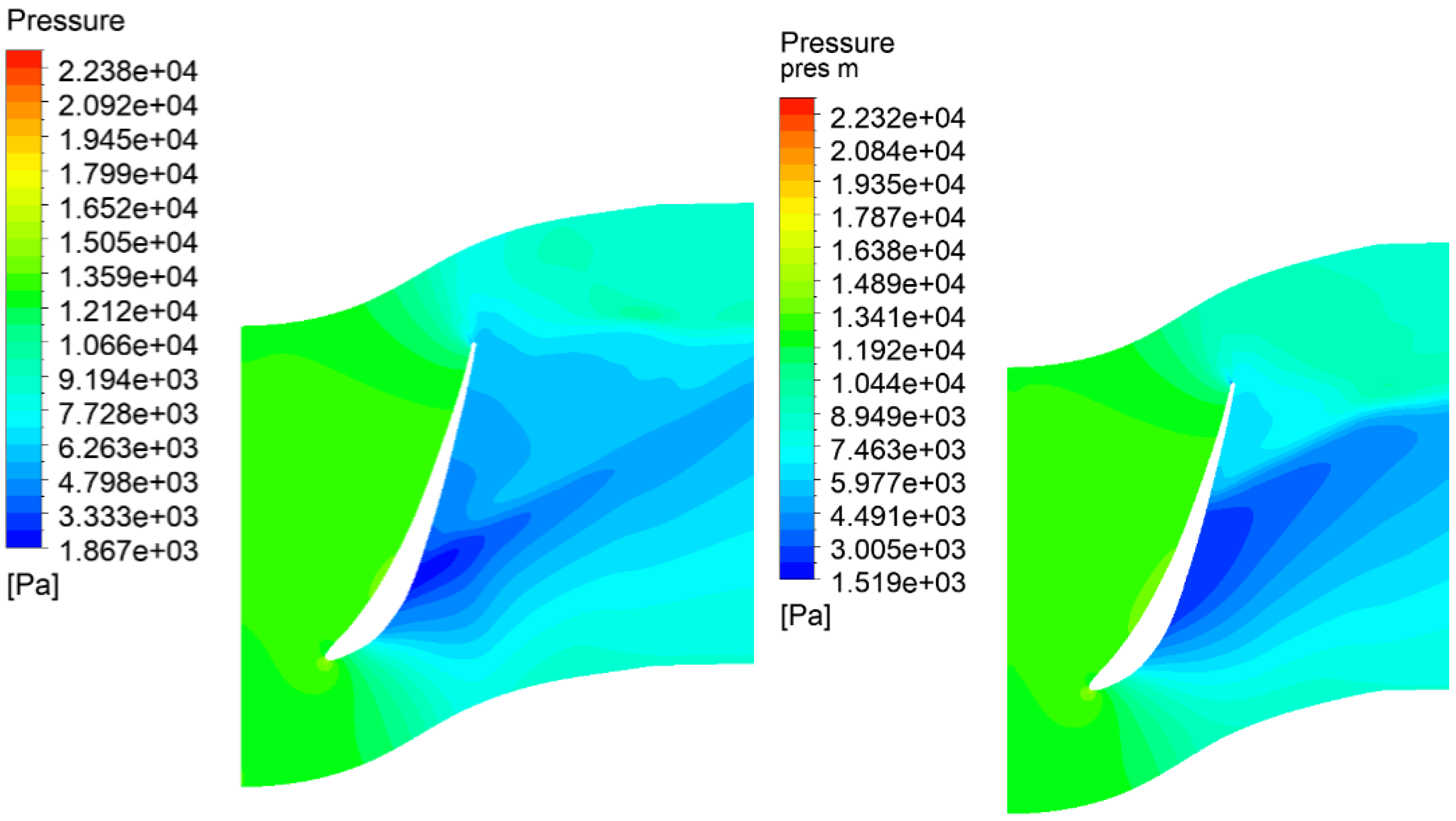
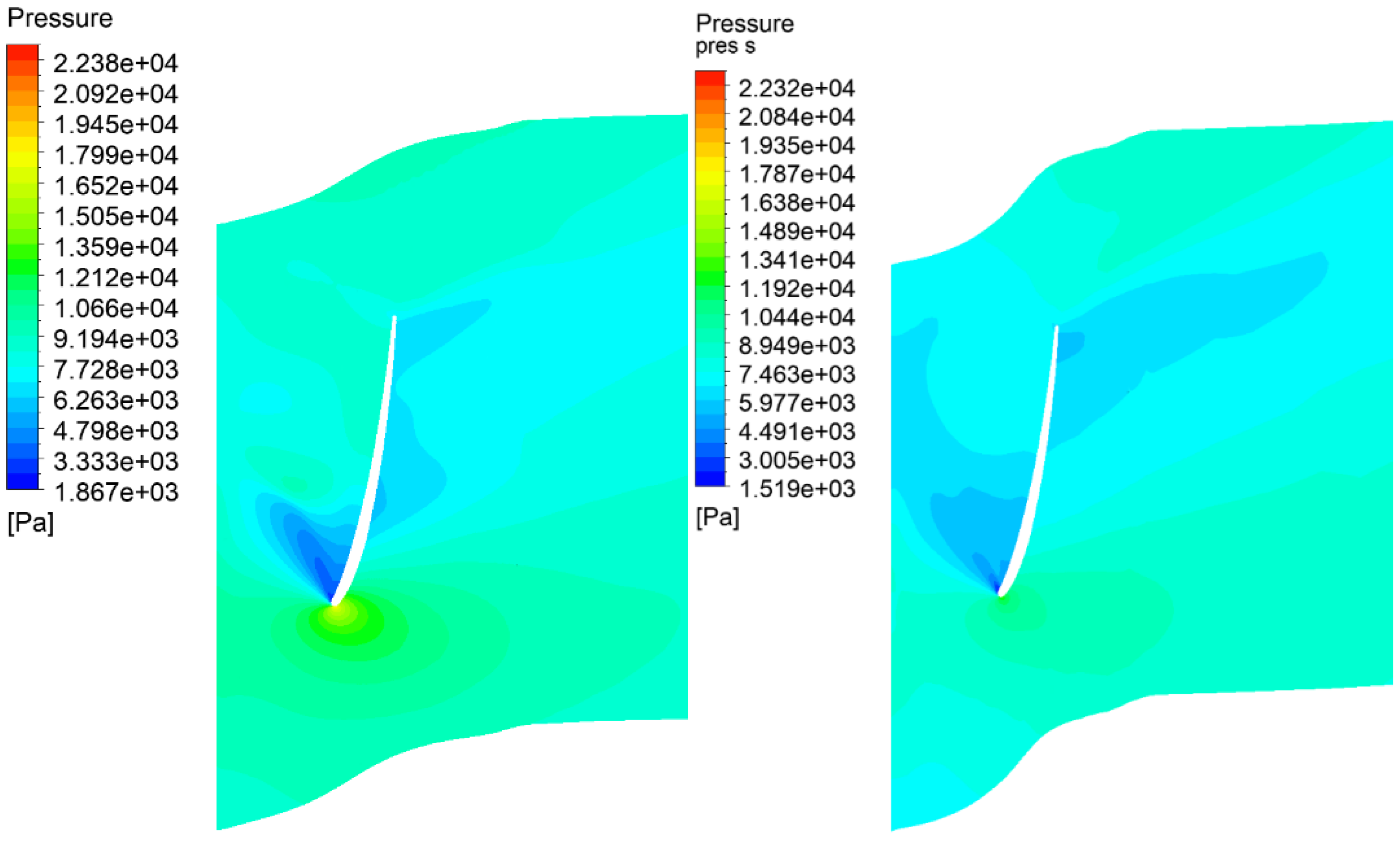
3.4. Comparison of Pressure

The loading profiles at the hub, at the mid-span, and at the shroud are presented in Figure 17, Figure 18 and Figure 19. It can be observed that the average pressure difference is increased. The largest improvement can be observed at the shroud (Figure 19). The pressure fields are presented in Figure 20, Figure 21 and Figure 22. Improved pressure fields can be seen, especially at the shroud in Figure 22, where the high-pressure area at the lower-pressure side of the blade is reduced. This change mostly leads to increased stage efficiency after optimization.

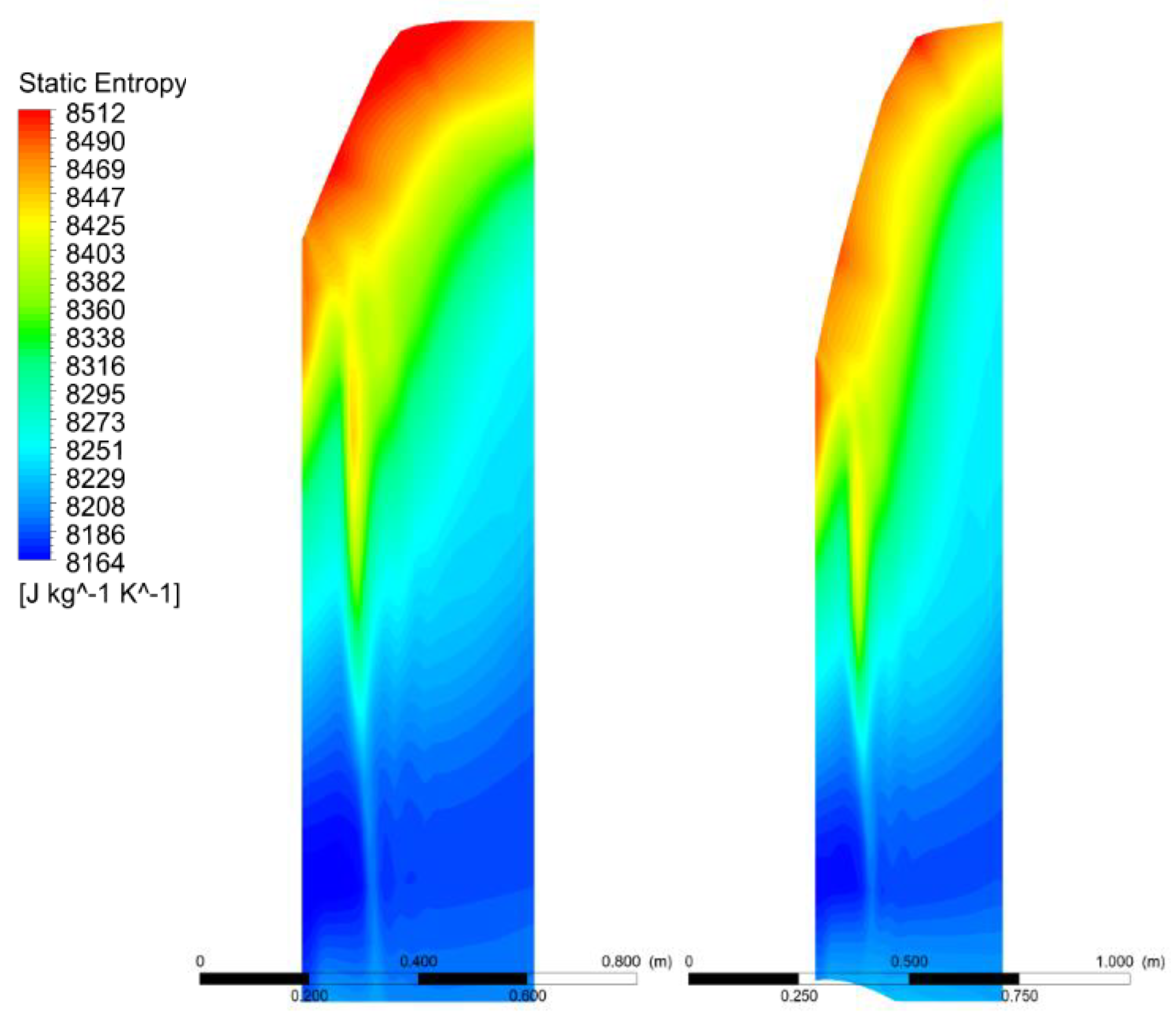
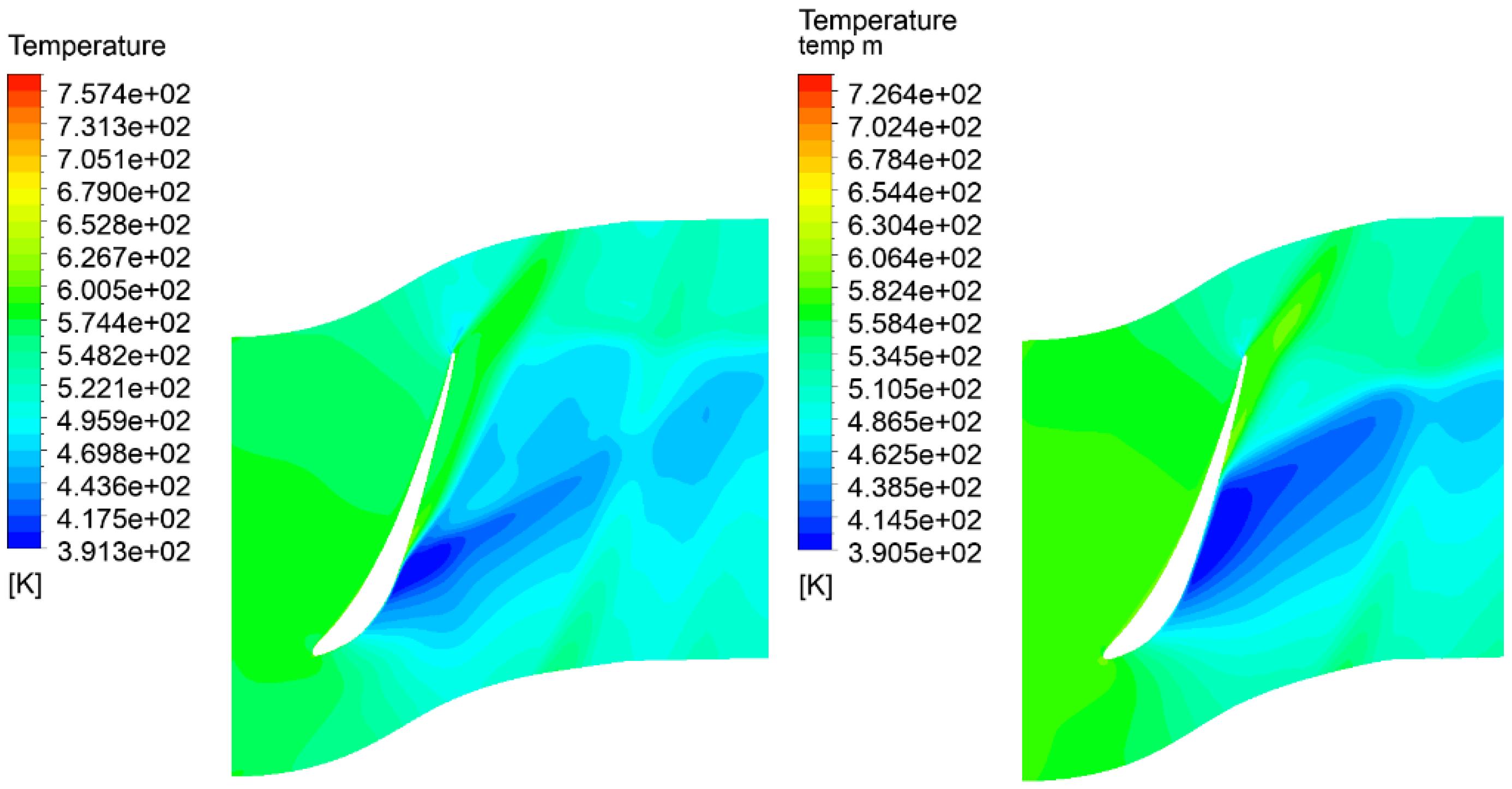
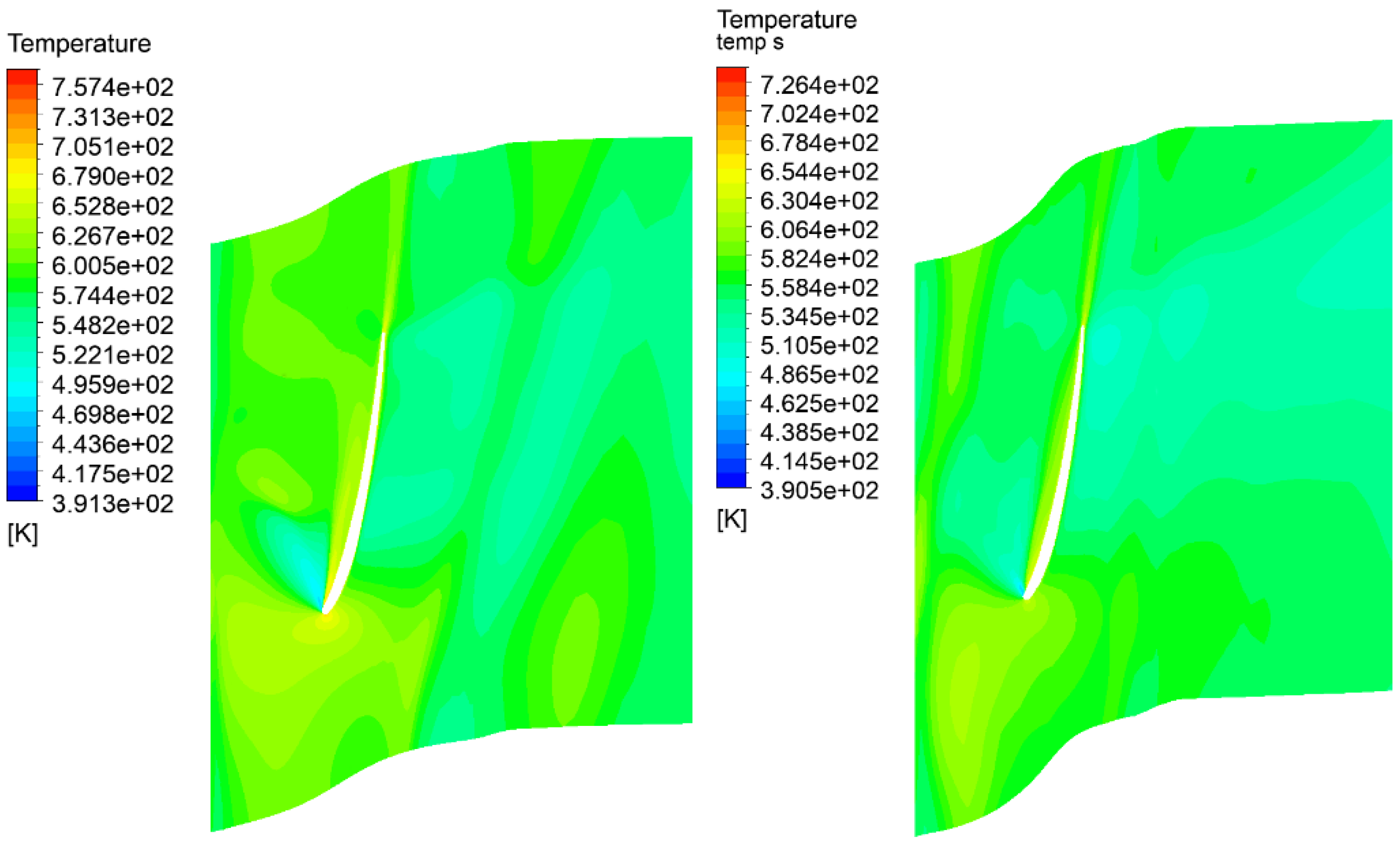
3.5. Comparison of Temperature

The temperature fields are presented in Figure 23, Figure 24, Figure 25 and Figure 26. The temperature at the last stage does not drop to the value of the saturation pressure of steam at a given pressure. However, this phenomena occurs in conventional steam turbines [66,67,68]. The key thermodynamic phenomena occurring in the flow of a gas–steam turbine concern the behavior of the mixture of fluids as the pressure drops during the transfer of mechanical energy to the turbine stages. As a result of the drop in enthalpy, the temperature also decreases, and the more efficient this process is, the lower the temperature obtained at the turbine outlet. However, the ratio between steam and carbon dioxide also affects the temperature decrease during this process, and it becomes apparent that a gas–steam turbine has smaller temperature decreases than a pure gas turbine. However, the advantage of the gas–steam turbine is that the thermodynamic expansion process can also be carried out to vacuum through the use of a condenser. In this case, the temperature can drop even to near-ambient values. However, the fluid dynamic phenomena occurring in the gas–steam mixture as it expands through the turbine stage is the same as in a classical steam turbine in superheated steam. Thus, droplet condensation would not occur in this type of turbine. An improvement in the temperature can be observed, especially at the rotor contours (Figure 23 and Figure 24), where a larger drop in temperature due to expansion can be observed. Simulations of the temperature fields can be used to compare them with measurements that allow the determination of the performance deterioration [69,70].

4. Conclusions and Perspectives

A technique described in previous articles by the authors [44,61,62] for the optimization of the shape has been used for the optimization of the axial and radial turbine stage. The flow efficiency of the last stage was improved by utilizing a hybrid algorithm termed HNMPSO. The abovementioned methods have not been applied in low-pressure turbine optimization working in a gas–steam cycle. The results demonstrate that this algorithm was successful in finding an optimal or close-to-optimal solution, resulting in reduced computational resources. The endwalls’ baseline geometry was created using a widely recognized aerodynamic method and was defined by two B-spline curves. The length of the last blade was slightly increased during the process of optimization (309.21 mm). This led to a rise of four percentage points in the total-to-static turbine efficiency due to the improved flow and a reduction in exit velocity losses.
As a result of the optimization in the rotor hub, there was a reduction in the separation zone. In the mid-span, on the other hand, the reverse vortices at the trailing edge disappeared. Next, in the shroud area at the leading edge, the fluid breakdown and strong flow turbulence were almost eliminated. Thus, the improvement in the nature of the flow was evident both in the velocity field and in the rotor blade loading diagrams. A particularly significant improvement was noted at the shroud, where two beneficial effects occurred. First, at the lower-pressure side, not only did the minimum pressure decrease from 5 kPa to 1.5 kPa, but also the pressure profile in the central part of the blade as well as at its trailing edge improved. There were no drifting pressure fields in the blade after optimization, resulting in an increase in the blade’s lifting force and the generation of more power; thus, higher efficiency, improved by four percentage points, was achieved.
In other words, the 4% change obtained during optimization corresponds to power of 0.549 MW. The kinetic energy of the working medium can be transferred during expansion in subsequent stages, but, after the last stage, there is no possibility to convert this output velocity. Thus, an optimal flow guarantees reduced losses at the turbine exit. The optimization process allowed for the reduction of vortices at the tip and, therefore, an improvement in the pressure fields affecting the rotor blade. This allowed us to increase the pressure difference acting on the blade and generate a higher power output while maintaining the rotational speed.
The high-quality results have been achieved by employing a mesh with over 20 million elements. In this case the percentage error in efficiency between the previous and current mesh sizes decreases below 0.05. However, it should be added that due to the increase in channel from 1812 mm to 2125 mm, the area in which the expansion takes place has increased, and a lower average outlet pressure of about 220.03 Pa has become possible. Average outlet temperature dropped by 36.5 K. Stator blade length changed from 1289 mm to 1297 mm and rotor blade increased from 1610 mm to 1791 mm.
The substantial improvement in the internal efficiency of the final stage has a direct impact on the overall system’s efficiency, as the kinetic energy cannot be reused after the last stage to generate additional work. The largest efficiency increase was observed near the shroud area presenting the profile loading. The flow separation from the blade was reduced at the mid-span and at the shroud.
The next step in the optimization process will involve expanding the number of parameters being optimized, including the blade number, stagger angle, and blade profile shape. The optimization will also consider the turbine’s performance under conditions that differ from the design regime. Another approach implemented in gas–steam turbines is fluid–solid interaction analysis, as well as the optimization of the blade profiles, including the stress level performance.
The system of the present dimensions could be used to decarbonize power generation in gas systems. The present turbine, once scaled up, could be particularly applicable to systems using renewable fuels, including biomass gasification. The main benefits, compared to other CO2 capture technologies, are the compactness of the present turbine and its ability to directly capture carbon dioxide by separation after water condensation.

Author Contributions

Conceptualization, P.Z., Ł.W., S.G., P.K., M.F. and A.K.; methodology, Ł.W. and P.K.; software, Ł.W. and S.G.; validation, Ł.W. and P.K.; formal analysis, Ł.W. and P.K.; investigation, Ł.W.; resources, Ł.W. and P.Z; data curation, S.G. and Ł.W.; writing—original draft preparation, S.G., P.Z. and Ł.W.; writing—review and editing, P.Z., S.G., P.K., M.F. and A.K.; visualization, S.G. and Ł.W.; supervision, P.Z.; project administration, P.Z.; funding acquisition, P.Z. All authors have read and agreed to the published version of the manuscript.

Funding

This research was funded by Gdańsk University of Technology, grant number DEC-50/2020/IDUB/I.3.3, under the ARGENTUM TRIGGERING RESEARCH GRANTS—EIRU program.

Data Availability Statement

The original contributions presented in the study are included in the article, further inquiries can be directed to the corresponding author.

Conflicts of Interest

The authors declare no conflict of interest.

References

  1. Głuch, J. Selected Problems of Determining an Efficient Operation Standard in Contemporary Heat-and-Flow Diagnostics. Pol. Marit. Res. 2009, 16, 22–26. [Google Scholar] [CrossRef]
  2. Kowalczyk, T.; Badur, J.; Bryk, M. Energy and exergy analysis of hydrogen production combined with electric energy generation in a nuclear cogeneration cycle. Energy Convers. Manag. 2019, 198, 111805. [Google Scholar] [CrossRef]
  3. Madejski, P.; Żymełka, P. Calculation methods of steam boiler operation factors under varying operating conditions with the use of computational thermodynamic modeling. Energy 2020, 197, 117221. [Google Scholar] [CrossRef]
  4. Dudda, W.; Banaszkiewicz, M.; Ziółkowski, P.J. Validation of a Burzyński plasticity model with hardening—A case of St12T. AIP Conf. Proc. 2019, 2077, 020016. [Google Scholar] [CrossRef]
  5. Badur, J.; Bryk, M. Accelerated start-up of the steam turbine by means of controlled cooling steam injection. Energy 2019, 173, 1242–1255. [Google Scholar] [CrossRef]
  6. Szewczuk-Krypa, N.; Grzymkowska, A.; Głuch, J. Comparative analysis of thermodynamic cycles of selected nuclear ship power plants with high-temperature helium-cooled nuclear reactor. Pol. Marit. Res. 2018, 25, 218–224. [Google Scholar] [CrossRef]
  7. Delgado-Torres, A.M.; García-Rodríguez, L. Analysis and optimization of the low-temperature solar organic Rankine cycle (ORC). Energy Convers. Manag. 2010, 51, 2846–2856. [Google Scholar] [CrossRef]
  8. Ziółkowski, P.; Głuch, S.; Ziółkowski, P.J.; Badur, J. Compact High Efficiency and Zero-Emission Gas-Fired Power Plant with Oxy-Combustion and Carbon Capture. Energies 2022, 15, 2590. [Google Scholar] [CrossRef]
  9. Głuch, S.J.; Ziółkowski, P.; Witanowski, Ł.; Badur, J. Design and Computational Fluid Dynamics Analysis of the Last Stage of Innovative Gas-Steam Turbine. Arch. Thermodyn. 2021, 42, 255–278. [Google Scholar] [CrossRef]
  10. Ziółkowski, P.; Witanowski; Klonowicz, P.; Głuch, S. Optimization of the Last Stage of Gas-Steam Turbine Using a Hybrid Method. In Proceedings of the 14th European Conference on Turbomachinery Fluid Dynamics and Thermodynamics, ETC 2021, Virtual, 12–16 April 2021; pp. 1–15. [Google Scholar]
  11. Martelli, E.; Alobaid, F.; Elsido, C. Design Optimization and Dynamic Simulation of Steam Cycle Power Plants: A Review. Front. Energy Res. 2021, 9, 676969. [Google Scholar] [CrossRef]
  12. Anderson, R.; Hustad, C.; Skutley, P.; Hollis, R. Oxy-Fuel Turbo Machinery Development for Energy Intensive Industrial Applications. Energy Procedia 2014, 63, 511–523. [Google Scholar] [CrossRef]
  13. Ziółkowski, P.; Głuch, S.; Kowalczyk, T.; Badur, J. Revalorisation of the Szewalski’s concept of the law of varying the last-stage blade retraction in a gas-steam turbine. E3S Web Conf. 2021, 323, 00034. [Google Scholar] [CrossRef]
  14. Dolatabadi, A.M.; Pour, M.S.; Ajarostaghi, S.S.M.; Poncet, S.; Hulme-Smith, C. Last stage stator blade profile improvement for a steam turbine under a non-equilibrium condensation condition: A CFD and cost-saving approach. Alex. Eng. J. 2023, 73, 27–46. [Google Scholar] [CrossRef]
  15. Turek, V.; Kilkovský, B.; Daxner, J.; Babička Fialová, D.; Jegla, Z. Industrial Waste Heat Utilization in the European Union—An Engineering-Centric Review. Energies 2024, 17, 2084. [Google Scholar] [CrossRef]
  16. Szewczuk-Krypa, N.; Drosińska-Komor, M.; Głuch, J.; Breńkacz, L. Comparison Analysis of Selected Nuclear Power Plants Supplied with Helium from High-Temperature Gas-Cooled Reactor. Pol. Marit. Res. 2018, 25, 204–210. [Google Scholar] [CrossRef]
  17. Mikielewicz, D.; Mikielewicz, J. Analytical Method for Calculation of Heat Source Temperature Drop for the Organic Rankine Cycle Application. Appl. Therm. Eng. 2014, 63, 541–550. [Google Scholar] [CrossRef]
  18. Micheli, D.; Pinamonti, P.; Reini, M.; Taccani, R. Performance Analysis and Working Fluid Optimization of a Cogenerative Organic Rankine Cycle Plant. ASME J. Energy Resour. Technol. 2013, 135, 021601. [Google Scholar] [CrossRef]
  19. Kupecki, J.; Motylinski, K.; Jagielski, S.; Wierzbicki, M.; Brouwer, J.; Naumovich, Y.; Skrzypkiewicz, M. Energy analysis of a 10 kW-class power-to-gas system based on a solid oxide electrolyzer (SOE). Energy Convers. Manag. 2019, 199, 111934. [Google Scholar] [CrossRef]
  20. Travieso Pedroso, D.; Blanco Machin, E.; Pérez, N.P.; Braga, L.B.; Silveira, J.L. Technical assessment of the Biomass Integrated Gasification/Gas Turbine Combined Cycle (BIG/GTCC) incorporation in the sugarcane industry. Renew Energy 2017, 114, 464–479. [Google Scholar] [CrossRef]
  21. Kotowicz, J.; Job, M.; Brzęczek, M. Thermodynamic Analysis and Optimization of an Oxy-Combustion Combined Cycle Power Plant Based on a Membrane Reactor Equipped with a High-Temperature Ion Transport Membrane ITM. Energy 2020, 205, 117912. [Google Scholar] [CrossRef]
  22. Ertesvåg, I.S.; Kvamsdal, H.M.; Bolland, O. Exergy Analysis of a Gas Turbine Combined-Cycle Power Plant With Precombustion CO2 Capture. Energy 2005, 30, 5–39. [Google Scholar] [CrossRef]
  23. Sadrian, V.; Lakzian, E.; Kim, H.D. Optimization of operating conditions in the stage of steam turbine by black-box method. Int. Commun. Heat Mass Transf. 2024, 155, 107499. [Google Scholar] [CrossRef]
  24. Nadirgil, O. Carbon price prediction using multiple hybrid machine learning models optimized by genetic algorithm. J. Environ. Manag. 2023, 342, 118061. [Google Scholar] [CrossRef]
  25. Sui, Y.; Chen, J.; Chu, P.; Lan, J.; Ren, S.; Wu, H.; Xu, Y.; Xie, J.; Ding, J. Aerodynamic optimization of the last stage turbine blade for an industrial gas turbine. IOP Conf. Ser. Mater. Sci. Eng. 2021, 1081, 012026. [Google Scholar] [CrossRef]
  26. Zheng, J.; Zhong, J.; Chen, M.; He, K. A reinforced hybrid genetic algorithm for the traveling salesman problem. Comput. Oper. Res. 2023, 157, 106249. [Google Scholar] [CrossRef]
  27. Lampart, P.; Hirt, Ł. Complex multidisciplinary optimization of turbine blading systems. Arch. Mech. 2012, 64, 153–175. [Google Scholar]
  28. Meng, M. A hybrid particle swarm optimization algorithm for satisficing data envelopment analysis under fuzzy chance constraints. Expert Syst. Appl. 2014, 41, 2074–2082. [Google Scholar] [CrossRef]
  29. Sundkvist, S.G.; Dahlquist, A.; Janczewski, J.; Sjödin, M.; Bysveen, M.; Ditaranto, M.; Langørgen, Ø.; Seljeskog, M.; Siljan, M. Concept for a combustion system in oxyfuel gas turbine combined cycles. J. Eng. Gas Turbine Power 2014, 136, 101513. [Google Scholar] [CrossRef]
  30. Rogalev, A.; Rogalev, N.; Kindra, V.; Komarov, I.; Zlyvko, O. Research and Development of the Oxy-Fuel Combustion Power Cycles with CO2 Recirculation. Energies 2021, 14, 2927. [Google Scholar] [CrossRef]
  31. Mathieu, P.; Nihart, R. Sensitivity analysis of the MATIANT cycle. Energy Convers. Manag. 1999, 40, 1687–1700. [Google Scholar] [CrossRef]
  32. Rogalev, A.; Rogalev, N.; Kindra, V.; Zlyvko, O.; Vegera, A. A Study of Low-Potential Heat Utilization Methods for Oxy-Fuel Combustion Power Cycles. Energies 2021, 14, 3364. [Google Scholar] [CrossRef]
  33. Hollis, R.; Skutley, P.; Ortíz, C.; Varkey, V.; Lepage, D.; Brown, B.; Davies, D.; Harris, M. Oxy-Fuel Turbomachinery Development for Energy Intensive Industrial Applications. In Proceedings of the ASME Turbo Expo 2012: Turbine Technical Conference and Exposition, Copenhagen, Denmark, 11–15 June 2012; pp. 431–439. [Google Scholar]
  34. Kiani, A.T.; Nadeem, M.F.; Ahmed, A.; Khan, I.A.; Alkhammash, H.I.; Sajjad, I.A.; Hussain, B. An improved particle swarm optimization with chaotic inertia weight and acceleration coefficients for optimal extraction of PV models parameters. Energies 2021, 14, 2980. [Google Scholar] [CrossRef]
  35. Ehteram, M.; Binti Othman, F.; Mundher Yaseen, Z.; Abdulmohsin Afan, H.; Falah Allawi, M.; Abdul Malek, M.B.; Najah Ahmed, A.; Shahid, S.; Singh, V.P.; El-Shafie, A. Improving the Muskingum flood routing method using a hybrid of particle swarm optimization and bat algorithm. Water 2018, 10, 807. [Google Scholar] [CrossRef]
  36. Yang, J.; Peng, T.; Xu, G.; Hu, W.; Zhong, H.; Liu, X. A Study and Optimization of the Unsteady Flow Characteristics in the Last Stage Impeller of a Small-Scale Multi-Stage Hydraulic Turbine. Energies 2023, 17, 107. [Google Scholar] [CrossRef]
  37. Lemmon, E.W.; Bell, I.H.; Huber, M.L.; McLinden, M.O. NIST Standard Reference Database 23: Reference Fluid Thermodynamic and Transport Properties-REFPROP, Version 10.0; National Institute of Standards and Technology: Gaithersburg, MD, USA, 2018. [Google Scholar] [CrossRef]
  38. Lampart, P.; Yershov, S.; Rusanov, A. Increasing Flow Efficiency of High-Pressure and Low-Pressure Steam Turbine Stages from Numerical Optimization of 3D Blading. Eng. Optim. 2005, 37, 145–166. [Google Scholar] [CrossRef]
  39. Lampart, P. Numerical Optimization of Stator Blade Sweep and Lean in an LP Turbine Stage. In Proceedings of the 2002 International Joint Power Generation Conference, Scottsdale, AZ, USA, 24–26 June 2002; pp. 579–592. [Google Scholar]
  40. Perycz, S. Steam and Gas Turbines, 1st ed.; Wydawnictwo Politechniki Gdańskiej: Gdańsk, Poland, 1988. [Google Scholar]
  41. Szewalski, R. A Novel Design of Turbine Blading of Extreme Length. Trans. Inst. Fluid-Flow Mach. 1976, 70–72, 83–86. [Google Scholar]
  42. Szewalski, R. Rational Blade Height Calculation in Action Turbines. Czas. Tech. 1930, 1, 83–86. [Google Scholar]
  43. Szewalski, R. Present Problems of Power Engineering Development. Increase of Unit Power and Efficiency of Turbines and Power Palnts; Ossolineum: Wrocław, Poland, 1978. [Google Scholar]
  44. Lampart, P.; Gardzilewicz, A.; Kwidzyński, R. On the Control of Flow Losses in LP Turbine Stages—Computation of Advanced Designs Based on a Solver of 3D Navier-Stokes Equations. In Proceedings of the Seminar Topical Problems of Fluid Mechanics, Prague, Czech Republic, 16 February 2000; pp. 53–56. [Google Scholar]
  45. Witanowski, Ł.; Klonowicz, P.; Lampart, P.; Suchocki, T.; Jędrzejewski, Ł.; Zaniewski, D.; Klimaszewski, P. Optimization of an Axial Turbine for a Small Scale ORC Waste Heat Recovery System. Energy 2020, 205, 118059. [Google Scholar] [CrossRef]
  46. ANSYS® Academic Research Mechanical and CFD, Release 19.0 2019; ANSYS Inc.: Canonsburg, PA, USA, 2019.
  47. Yang, X.-S. Recent Advances in Swarm Intelligence and Evolutionary Computation; Springer: Cham, Switzerland, 2015; ISBN 978-3-319-13825-1. [Google Scholar]
  48. Ting, T.O.; Yang, X.-S.; Cheng, S.; Huang, K. Hybrid Metaheuristic Algorithms: Past, Present, and Future; Studies in Computational Intelligence; Springer: Cham, Switzerland, 2015; Volume 585, pp. 71–83. ISBN 9783319138268. [Google Scholar]
  49. Tesch, K.; Kaczorowska-Ditrich, K. The Discrete-Continuous, Global Optimisation of an Axial Flow Blood Pump. Flow Turbul. Combust. 2020, 104, 777–793. [Google Scholar] [CrossRef]
  50. Eberhart, R.; Kennedy, J. New Optimizer Using Particle Swarm Theory. In Proceedings of the Sixth International Symposium on Micro Machine and Human Science (MHS’95), Nagoya, Japan, 4–6 October 1995; pp. 39–43. [Google Scholar] [CrossRef]
  51. Nelder, J.A.; Mead, R. A Simplex Method for Function Minimization. Comput. J. 1965, 7, 308–313. [Google Scholar] [CrossRef]
  52. Zahara, E.; Kao, Y.T. Hybrid Nelder-Mead Simplex Search and Particle Swarm Optimization for Constrained Engineering Design Problems. Expert Syst. Appl. 2009, 36, 3880–3886. [Google Scholar] [CrossRef]
  53. Fan, S.K.S.; Zahara, E. A Hybrid Simplex Search and Particle Swarm Optimization for Unconstrained Optimization. Eur. J. Oper. Res. 2007, 181, 527–548. [Google Scholar] [CrossRef]
  54. Ayouche, S.; Ellaia, R.; Aboulaich, R. A Hybrid Particle Swarm Optimization-Nelder- Mead Algorithm (PSO-NM) for Nelson-Siegel- Svensson Calibration. Int. J. Econ. Manag. Eng. 2016, 10, 1365–1369. [Google Scholar] [CrossRef]
  55. Barzinpour, F.; Noorossana, R.; Niaki, S.T.A.; Ershadi, M.J. A Hybrid Nelder–Mead Simplex and PSO Approach on Economic and Economic-Statistical Designs of MEWMA Control Charts. Int. J. Adv. Manuf. Technol. 2013, 65, 1339–1348. [Google Scholar] [CrossRef]
  56. Tsai, H.H.; Fuh, C.C.; Ho, J.R.; Lin, C.K. Design of Optimal Controllers for Unknown Dynamic Systems through the Nelder–Mead Simplex Method. Mathematics 2021, 9, 2013. [Google Scholar] [CrossRef]
  57. Ma, Y.; Zhang, A.; Yang, L.; Hu, C.; Bai, Y. Investigation on optimization design of offshore wind turbine blades based on particle swarm optimization. Energies. 2019, 12, 1972. [Google Scholar] [CrossRef]
  58. Sulaiman, A.T.; Bello-Salau, H.; Onumanyi, A.J.; Mu’azu, M.B.; Adedokun, E.A.; Salawudeen, A.T.; Adekale, A.D. A Particle Swarm and Smell Agent-Based Hybrid Algorithm for Enhanced Optimization. Algorithms 2024, 17, 53. [Google Scholar] [CrossRef]
  59. Rong, L.; Böhle, M.; Yandong, G. Improving the hydraulic performance of a high-speed submersible axial flow pump based on CFD technology. Int. J. Fluid Eng. 2024, 1, 013902. [Google Scholar] [CrossRef]
  60. Zanetti, G.; Siviero, M.; Cavazzini, G.; Santolin, A. Application of the 3D inverse design method in reversible pump turbines and Francis turbines. Water 2023, 15, 2271. [Google Scholar] [CrossRef]
  61. Witanowski, Ł.; Klonowicz, P.; Lampart, P.; Klimaszewski, P.; Suchocki, T.; Jędrzejewski, Ł.; Zaniewski, D.; Ziółkowski, P. Impact of Rotor Geometry Optimization on the Off-Design ORC Turbine Performance. Energy 2023, 265, 126312. [Google Scholar] [CrossRef]
  62. Witanowski, Ł.; Klonowicz, P.; Lampart, P.; Ziółkowski, P. Multi-Objective Optimization of the ORC Axial Turbine for a Waste Heat Recovery System Working in Two Modes: Cogeneration and Condensation. Energy 2023, 264, 126187. [Google Scholar] [CrossRef]
  63. Zhao, J.; Pei, J.; Yuan, J.; Wang, W. Structural optimization of multistage centrifugal pump via computational fluid dynamics and machine learning method. J. Comput. Des. Eng. 2023, 10, 1204–1218. [Google Scholar] [CrossRef]
  64. Zych, P.; Żywica, G. Optimisation of stress distribution in a highly loaded radial-axial gas microturbine using FEM. Open Eng. 2020, 10, 318–335. [Google Scholar] [CrossRef]
  65. Zych, P.; Żywica, G. Fatigue analysis of the microturbine rotor disc made of 7075 aluminium alloy using a new hybrid calculation method. Materials 2022, 15, 834. [Google Scholar] [CrossRef]
  66. Fan, S.; Wang, Y.; Yao, K.; Shi, J.; Han, J.; Wan, J. Distribution characteristics of high wetness loss area in the last two stages of steam turbine under varying conditions. Energies 2022, 15, 2527. [Google Scholar] [CrossRef]
  67. Dykas, S.; Majkut, M.; Smołka, K.; Strozik, M. Study of the wet steam flow in the blade tip rotor linear blade cascade. Int. J. Heat Mass Transf. 2018, 120, 9–17. [Google Scholar] [CrossRef]
  68. Han, Z.; Zeng, W.; Han, X.; Xiang, P. Investigating the dehumidification characteristics of turbine stator cascades with parallel channels. Energies 2018, 11, 2306. [Google Scholar] [CrossRef]
  69. Głuch, J. Fault detection in measuring systems of power plants. Pol. Marit. Res. 2008, 18, 45–51. [Google Scholar] [CrossRef]
  70. Gluch, J.; Krzyzanowski, J. New Attempt for Diagnostics of the Geometry Deterioration of the Power System Based on Thermal Measurement. In Proceedings of the ASME Turbo Expo 2006: Power for Land, Sea, and Air, Barcelona, Spain, 8–11 May 2006; pp. 531–539. [Google Scholar]
Figure 1. The thermodynamic cycle of a gas–steam turbine with the cross-section of a low-pressure turbine, where HP and LP denote the gas turbine divided into two parts, high and low pressure, respectively. 1–16 nodes points in thermodynamic cycle.
Energies 17 02816 g001
Figure 2. Stator and rotor: (a) view from top and front, (b) view of stator–rotor blade configuration, (c) blade cross-section for specific meridional contour, (d) angles for different levels, hub (h) and shroud (s), respectively.
Energies 17 02816 g002
Figure 3. Optimization scheme.
Energies 17 02816 g003
Figure 4. Meridional contours of rotor row (the arrows indicate the direction of change in the decision variables).
Energies 17 02816 g004
Figure 5. Mesh used in numerical simulation: (a) relative difference between mean values of total-to-static efficiency with respect to finest investigated grid; (b) iteration loop; and (c) verification phase (finest grid of 20 mln nodes).
Energies 17 02816 g005
Figure 6. Objective function vs. function evaluation during the optimization process.
Energies 17 02816 g006
Figure 7. Base (original) and final values of the efficiency.
Energies 17 02816 g007
Figure 8. Static entropy contours in the rotor: original design (left), optimized design (right).
Energies 17 02816 g008
Figure 9. Comparison of the original and optimized meridional section of the last turbine stage.
Energies 17 02816 g009
Figure 10. Velocity vectors in the rotor at the hub: original design (above), optimized design (below). The marked area shows separation in the form of velocity vectors (in the red square).
Energies 17 02816 g010
Figure 11. Velocity vectors in the rotor at the mid-span: baseline design (above), optimized design (below). The red square shows separation and a reverse vortex.
Energies 17 02816 g011
Figure 12. Velocity vectors in the rotor at the shroud: baseline design (above), optimized design (below). In the red square, a non-optimized angle of attack on the blade is highlighted, causing fluid breakdown and turbulence.
Energies 17 02816 g012
Figure 13. Mach number in the rotor at the hub: baseline design (above), optimized design (below). Visible separation of the fluid from the blade on the suction side in the form of a pressure drop (in the red square).
Energies 17 02816 g013
Figure 14. Mach number in the rotor at the mid-span: baseline design (above), optimized design (below). The red squares show a shock wave forming on the suction side and significant breakaway at the trailing edge, causing flow losses.
Energies 17 02816 g014
Figure 15. Mach number in the rotor at the shroud: baseline design (above), optimized design (below). The square indicates the inappropriate distribution of the Mach number on the suction side with lowered pressure, contributing to the inappropriate pressure profiles.
Energies 17 02816 g015
Figure 16. Streamlines in the stage: baseline design (above), optimized design (below). Significant vortex structures causing suboptimal inflow angles at the leading edge of the rotor blade are marked in the square. This type of turbulence causes ventilator operation and significant entropy generation due to the reduced mechanical work output.
Energies 17 02816 g016
Figure 17. Rotor blade loading at the hub.
Energies 17 02816 g017
Figure 18. Rotor blade loading at the mid-span.
Energies 17 02816 g018
Figure 19. Rotor blade loading at the shroud.
Energies 17 02816 g019
Figure 20. Pressure contours in the rotor at the hub: baseline design (left), optimized design (right).
Energies 17 02816 g020
Figure 21. Pressure contours in the rotor at the mid-span: baseline design (left), optimized design (right).
Energies 17 02816 g021
Figure 22. Pressure contours in the rotor at the shroud: baseline design (left), optimized design (right).
Energies 17 02816 g022
Figure 23. Temperature contours in the rotor: baseline design (left), optimized design (right).
Energies 17 02816 g023
Figure 24. Temperature contours in the rotor at the hub: baseline design (left), optimized design (right).
Energies 17 02816 g024
Figure 25. Temperature contours in the rotor at the mid-span: baseline design (left), optimized design (right).
Energies 17 02816 g025
Figure 26. Temperature contours in the rotor at the shroud: baseline design (left), optimized design (right).
Energies 17 02816 g026
Table 1. Boundary conditions for CFD simulation of last turbine stage.
t inlet last stage = 336.794°C
m inlet last stage = 91.15kg/s
p outlet last stage = 0.07955bar
ω = 3000.rpm
XCO2XH2OXN2Sum
0.08940.90840.00221
YCO2YH2OYN2Sum
0.19330.80370.0031
Table 2. Parameters of twisted stage geometry at different heights.
Parameter Unit1 = Hub23 = Mid span45 = Shroud
r 1 m0.86321.12181.46671.81162.0703
r 2 m0.87271.18831.60912.032.3455
ρ -0.19060.52210.71520.80840.8503
u m/s274.17373.32505.52637.72736.87
α 1 °14.66119.00824.9530.08933.623
c 1 s m/s529.8413.9328.02277.18251.01
c 1 m/s495.38393.2311.6263.32238.46
β 2 °20.98819.12716.47613.86112.262
Disclaimer/Publisher’s Note: The statements, opinions and data contained in all publications are solely those of the individual author(s) and contributor(s) and not of MDPI and/or the editor(s). MDPI and/or the editor(s) disclaim responsibility for any injury to people or property resulting from any ideas, methods, instructions or products referred to in the content.

