Article

TensorRT Powered Model for Ultra-Fast Li-Ion Battery Capacity Prediction on Embedded Devices

1
College of Engineering Training Centre, China Jiliang University, Hangzhou 310018, China
2
School of Electronics and Information Engineering, Hangzhou Dianzi University, Hangzhou 310018, China
*
Author to whom correspondence should be addressed.
Energies 2024, 17(12), 2797; https://doi.org/10.3390/en17122797
Submission received: 9 March 2024 / Revised: 12 April 2024 / Accepted: 28 May 2024 / Published: 7 June 2024
(This article belongs to the Section K: State-of-the-Art Energy Related Technologies)

Abstract

:
The LSTM neural network is often employed for time-series data prediction due to its strong nonlinear mapping capability and memory effect, allowing for better identification of complex data characteristics. However, the large computational workload required by neural networks can result in longer prediction times, making deployment on time-sensitive embedded devices challenging. To address this, TensorRT, a software development kit for NVIDIA hardware platforms, offers optimized network structures and reduced inference times for deep learning inference applications. Though TensorRT inference is GPU-based like other deep learning frameworks, TensorRT outperforms comparable frameworks in terms of inference speed. In this paper, we compare the inference time consumption and prediction deviation of various approaches on CPU, GPU, and TensorRT, while also exploring the effects of different quantization approaches. Our experiments demonstrate the accuracy and inference latency of the same model on the FPGA development board PYNQ-Z1 as well, though the best results were obtained using NVIDIA Jetson Xavier NX. The results show an approximately 50× improvement in inference speed compared to our previous technique, with only a 0.2% increase in Mean Absolute Percentage Error (MAPE). These works highlight the effectiveness and efficiency of TensorRT in reducing inference times, making it an excellent choice for time-sensitive embedded device deployments that require high precision and low latency.

1. Introduction

Lithium-ion (Li-ion) batteries have been widely popular in the automotive and aerospace fields, among others, owing to their advantages such as non-pollution and high power density, as noted by [1,2,3]. During the continuous charge and discharge cycles, different chemical reactions take place inside the battery, causing gradual degradation of its performance. Therefore, to ensure the safety and reliability of Li-ion batteries, the monitoring of the external state is necessary to predict the internal state accurately. However, as pointed out by [4], the battery degradation process is complex, and battery degradation curves of various types and compositions are not consistently parallel, making the accurate prediction of internal battery states a challenging problem. Refs. [5,6,7] have made significant efforts to develop battery life prediction models, such as semi-empirical and electrochemical models. Despite these significant efforts, the estimation and prediction of the battery’s performance in real-world applications still present significant biases.
As an indicator of the aging status of Li-ion batteries, the state of health (SOH) is usually defined by one of two metrics: remaining capacity and internal resistance. End of life (EOL) is then defined as the end point of battery life when the chosen SOH metric crosses a certain threshold, often with the original value of remaining capacity at 80% and internal impedance at 200%. Accurate SOH estimation is crucial for the operation, maintenance, and optimization of batteries, but monitoring the aging is a very challenging task due to the complex and nonlinear mechanisms that cause battery aging. There are multiple aging mechanisms that interact and promote different aging modes, which lead to battery aging through complex degradation pathways.
Numerous methodologies for evaluating the condition of battery health have been expounded upon in the literature, as chronicled by the esteemed author [8]. The predominant method for assessing battery health entails controlled experimentation, employing techniques such as Coulomb counting or more sophisticated methodologies like electrochemical impedance spectroscopy (EIS) and incremental capacity and differential voltage (IC/DV) analysis. An evident limitation of these methodologies is their dependence on a distinct current profile, a formidable challenge in real-world operational environments. For example, IC/DV analysis emulates equilibrium conditions through the utilization of charge–discharge curves obtained by applying exceedingly low currents to the battery. These curves are subsequently subjected to differentiation to generate IC/DV plots. Despite the implementation of smoothing filters, differentiation amplifies noise effects, necessitating data collection over a wide voltage spectrum—a formidable endeavor in practical circumstances. To surmount these constraints, methodologies capable of harnessing sensor data routinely gathered from operational batteries are indispensable. In particular, time-series sensor data derived from the battery’s habitual charge–discharge pattern prove advantageous for estimation techniques that do not perturb the battery’s normal operation.
The most widely used SOH estimation method in industry is the parametric battery model, typically implemented through techniques such as the Kalman filter. Models can take a variety of forms, such as equivalent circuit models or electrochemical models. Circuit models define a circuit with various components to simulate the battery’s electrodynamic, while electrochemical models use a series of coupled partial differential equations to represent the distribution of Li-ion concentration and potential within the battery. However, these methods are limited in their accuracy, which highly depends on the selected underlying battery model.
With the ever-expanding field of artificial intelligence, several new methods have emerged for battery SOH estimation that can provide more accurate results. In particular, Recurrent Neural Networks (RNNs), widely used in domains concerned with time-series data, have become quite popular for applications such as speech recognition, video streaming analysis, and text processing. However, RNNs, comprising sigma units or tanh units, do not establish correlation of input data seamlessly when a large input gap exists. Long Short-Term Memory (LSTM) was introduced with gate functions in the cell structure, which can handle the problem of long-term dependence excellently. Since its inception, LSTM has demonstrated good results in predicting complex time-series data and emerged as the most popular time-series prediction algorithm. For example, ref. [9] designed bidirectional LSTM networks for sound classification and recognition. Similarly, ref. [10] used CNN-LSTM networks for predicting air pollution, while [11] predicted traffic flow by using CNN-LSTM networks. Additionally, ref. [12] used LSTM networks to predict wind speed and control the operation of wind turbines to ensure stable power systems. These findings suggest that LSTM networks have been widely used for time series prediction.
In recent years, academics have explored methods to enable model deployment and hardware acceleration to ensure large models can be deployed in embedded scenarios. For instance, ref. [13] proposed a parallelization approach to maximize the throughput of a single DL application using GPUs and NPUs. They demonstrated that exploiting various types of parallelism with TensorRT greatly increased processing speed. Similarly, ref. [14] proposed an efficient Dual Integrated Convolutional Neural Network (DICNN) model for real-time recognition of facial expressions. By using an embedded platform, this 1.08 M parameter model maintained a good balance between recognition accuracy and computational efficiency. Furthermore, ref. [15] proposed the use of TensorRT, an NVIDIA acceleration technology, to enhance processing speed and computational efficiency on a mobile quadruped robot platform.
Inspired by [16,17,18] studies, we designed an LSTM network to predict battery capacity from measured voltage, current, and temperature values. We trained and tested the model to obtain accurate prediction results. However, because of the low computing power of embedded devices and the high computational needs of neural networks, this model cannot be deployed on such devices. In certain applications, such as those involving embedded devices, shorter inference latency is frequently preferred over smaller inference deviation.
Nowadays, deep learning inference is widely used in embedded devices, and such devices are equipped with GPUs, NPUs, and other accelerators. For example, Jetson Xavier NX contains a CPU and a GPU. As the GPU provides more parallel computation units than a CPU, inferencing on the GPU is multiple times faster than on the CPU. This makes it possible to deploy highly accurate models on embedded devices on a large scale.
To enable model deployment in embedded devices, refs. [19,20,21] have attempted to optimize models using hardware acceleration techniques such as using GPUs and NPUs, as well as by using optimization techniques.
Several researchers have attempted to accelerate neural network inference using FPGAs. Refs. [22,23,24,25] have explored the use of Xilinx Zynq FPGAs to deploy models and achieve significant optimization. These studies highlight the effectiveness of utilizing FPGAs for accelerating deep learning inference, particularly in edge computing scenarios where low latency and high throughput are critical. With the ability to perform parallel computations and handle large amounts of data, FPGAs present a promising solution for real-time applications that require high performance and low power consumption.
In this paper, we attempted to deploy our model on the FPGA development board, but more focused on accelerating and optimizing it using CPU, GPU, TensorRT, and various quantization techniques, achieving a better balance of latency and accuracy for embedded scenarios. This allows our model to provide fast, stable, and accurate results on embedded devices, especially in time-sensitive scenarios. With a total of eight tests on the training and testing sets, our model achieved significant speedup of up to 50×, while the increase in mean absolute percentage error (MAPE) was only 0.2%. Our results demonstrate the importance of hardware acceleration and model quantization for accelerating model inference speed in embedded devices. Although our proposed optimization scheme is currently validated only on specific hardware platforms, we believe that these optimization techniques can be applied to other neural networks and hardware platforms.

2. Data Preparation and Model Composition

2.1. Data Preparation

We utilized the dataset from [26]. Figure 1 provides an overview of the dataset. The dataset comprised 28 individual cells that were classified into seven distinct test groups (Group 1: cells #5–#7, #18; Group 2: cells #25–#28; Group 3: cells #29–#32; Group 4: cells #33, #34, #36; Group 5: cells #38–#40; Group 6: cells #41–#44; Group 7: cells #45–#48; Group 8: cells #49–#52; and Group 9: cells #53–#56.), according to specific protocols and procedures. Table 1 provides a detailed overview of the conditions under which these batteries were tested.
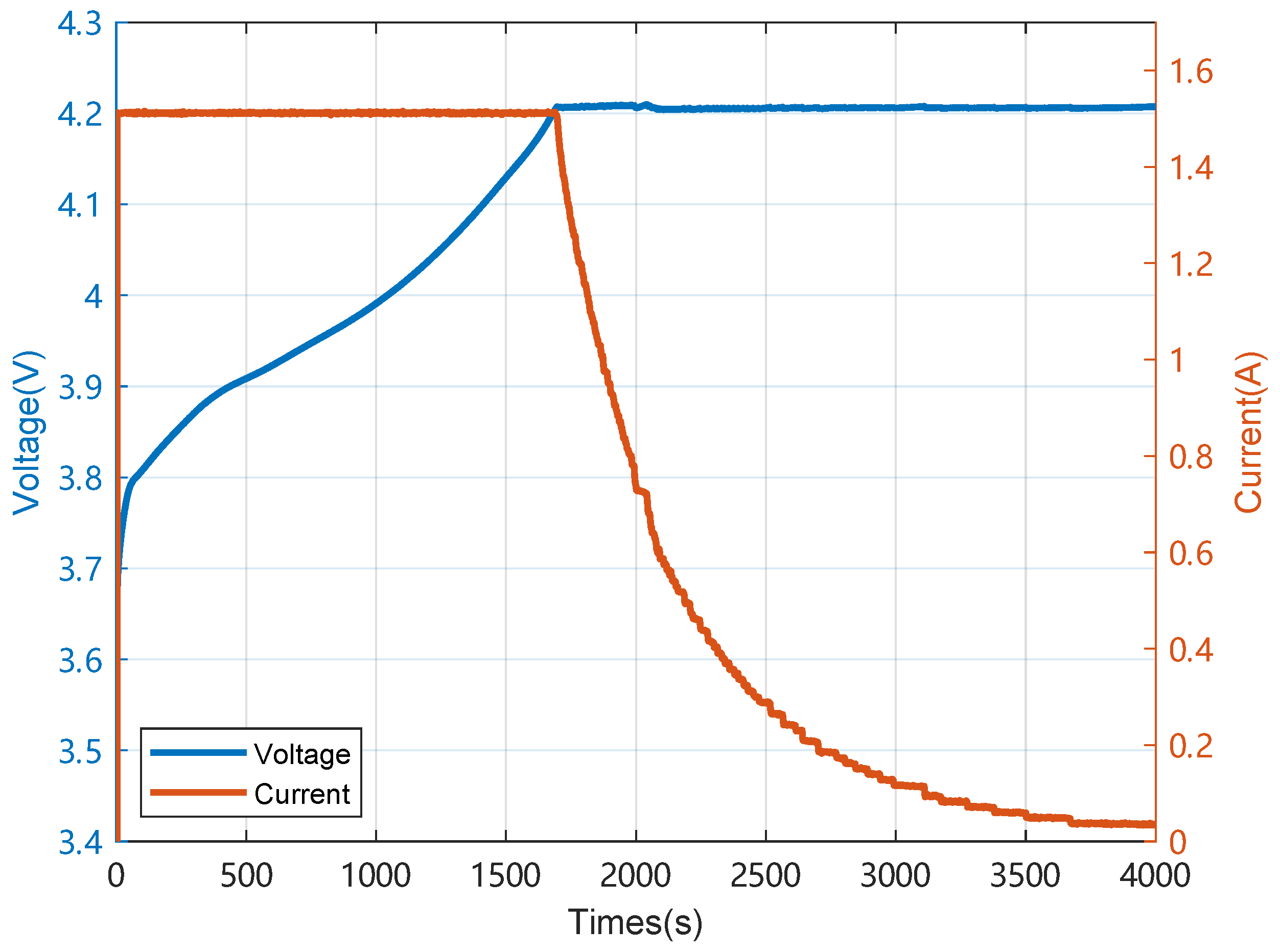
The charging process consisted of two modes: constant current (CC) mode and constant voltage mode. A constant current of 1.5 A was applied in CC mode until the voltage reached 4.2 V. This was followed by constant voltage mode until the current declined to 20 mA.
Different discharge modes were adopted for various batteries. Batteries #5, #6, #7, and #18 underwent a constant current discharge of 1 C. These batteries were discharged at a constant current level of 2 A until the battery voltage fell to 2.7 V, 2.5 V, 2.2 V, and 2.5 V, respectively, at room temperature. In contrast, four Li-ion batteries (#29, #30, #31, and #32) were subjected to elevated ambient temperature (43 °C), and discharge was performed at 4 A until the battery voltage dropped to 2.0 V, 2.2 V, 2.5 V, and 2.7 V.
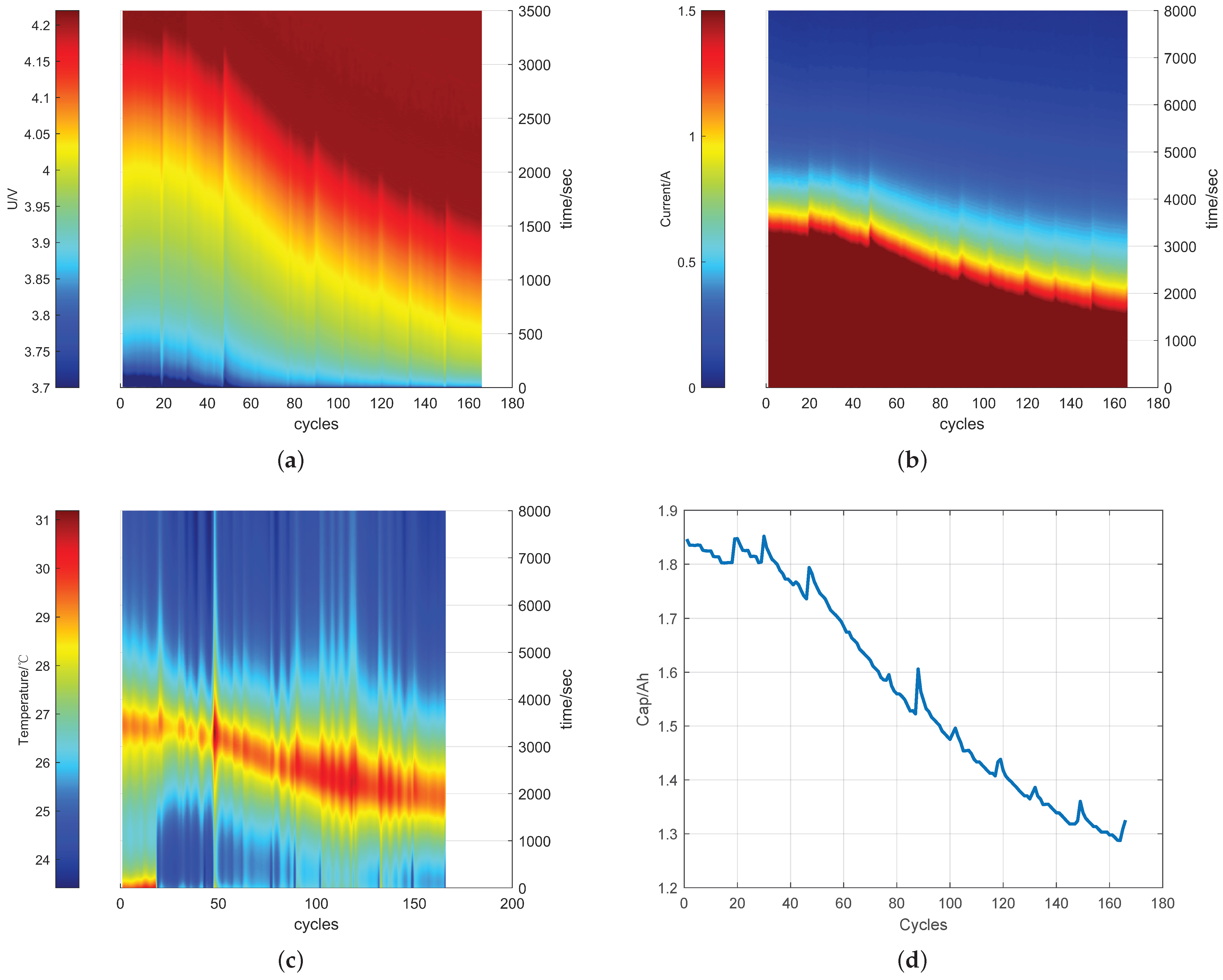
Figure 2 presents four charts illustrating the aging process of Battery #5. Figure 2a shows the charging voltage curve, which depicts a gradual increase in voltage until it reaches 4.2 V at the end of the constant current charging mode. Afterward, the voltage remains stable during constant voltage charging mode until the current drops to 20 mA. Figure 2b displays the charging current curve, which reveals a decrease in current along with the increase in voltage during the constant current charging mode. The current then remains stable during the constant voltage charging mode until it reaches 20 mA. Figure 2c illustrates the charging temperature curve, which indicates an initial increase in temperature during the constant current charging mode and a decrease during constant voltage charging mode. Finally, the temperature stabilizes during the rest period. Figure 2d depicts the capacity degradation curve, showing a gradual decline in capacity over time.
Additionally, three Li-ion batteries (#38, #39, and #40) were tested under multiple ambient temperatures (24 and 44 °C), using multiple load current levels (1 A, 2 A, and 4 A), and discharged at 2.2 V, 2.5 V, and 2.7 V. Finally, four Li-ion batteries (#45, #46, #47, and #48) were run under an ambient temperature of 4 °C with a fixed load current level of 1 A, and the discharge runs were stopped at 2 V, 2.2 V, 2.5 V, and 2.7 V.
In this paper, we focused on four Li-ion batteries (#5, #6, #7, #18), each with a nominal capacity of 2 Ah, that were subjected to loop charging and discharging at a constant temperature of 24 °C. The terminal voltage data and the battery life cycle capacity data were collected during the constant current charging process. Subsequently, the data underwent normalization processing to divide them into three groups: training data, validation data and testing data.
In the process of constant current charging, the variation of terminal voltage during battery aging is depicted as shown in Figure 3. It can be observed from Figure 2 that the overall trend of the battery terminal voltage variation curve remains consistent during each charging process. However, after undergoing several charge–discharge cycles, the initial values of the battery terminal voltage have changed. Furthermore, Figure 2 prominently highlights that in the aging experiment, the initial terminal voltages of the four batteries do not completely overlap on the same curve. It can be inferred that during the constant current charging phase, the battery’s terminal voltage curve will exhibit characteristics related to SOH. A specialized battery testing equipment collected a total of 1138 sets of data, each set including 4000 voltage points, 4000 current points, and 4000 temperature points. The data were randomly selected, with 70% of the data used for training, 20% for validation, and the remaining 10% allocated to the testing set.

2.2. LSTM Network Structure

The LSTM cells are interconnected to form a longer LSTM network. The connections are shown in Figure 4.
The key component of an LSTM cell is the cell state, as shown in Figure 4. The cell state is a horizontal line that runs from left to right across the top of the cell. It acts as a transmission line to pass critical information from one cell to the next, while having minimal, linear interactions with the rest of the cell.
To achieve the function of forgetting or memorization, the LSTM network implements “Gates”. These gates are designed to allow the selective flow of information and consist of a sigmoid function and a dot product operation. The sigmoid function has an output value in the range of [ 0 , 1 ] , where 0 indicates complete discard and 1 indicates complete pass-through. An LSTM cell generally includes three types of gates: forget gate, input gate, and output gate, as illustrated in Figure 5.
  • The structure of the forget gate, shown in Figure 5a, comprises a sigmoid function that takes as input both the output h t 1 of the previous cell and the input x t of the present cell. The output value of this sigmoid function falls within the range of [ 0 , 1 ] for each element in C t 1 , serving to regulate the extent to which the cell’s previous status is forgotten.
  • The structure of the input gate, shown in Figure 5b, interacts with a tanh function to determine which new information should be incorporated. The output of the tanh function results in a new candidate vector. Combining the output of the “forget gate”, which governs the amount of the previous cell that is forgotten, with the output of the input gate, which controls how much new information is incorporated, we obtain an updated status for the memory cell. Consequently, the output of the “forget gate” regulates the degree to which the previous cell is forgotten, and the output of the “input gate” determines how much new information is integrated. Based on these two outputs, the cell status can be updated.
  • The structure of the output gate, shown in Figure 5c, is used to filter out the current cell state to a certain extent. First, cell states are activated, and then the output gate generates a value within the range of [ 0 , 1 ] for each state, controlling the degree to which the cell state is filtered.

2.3. Model Composition

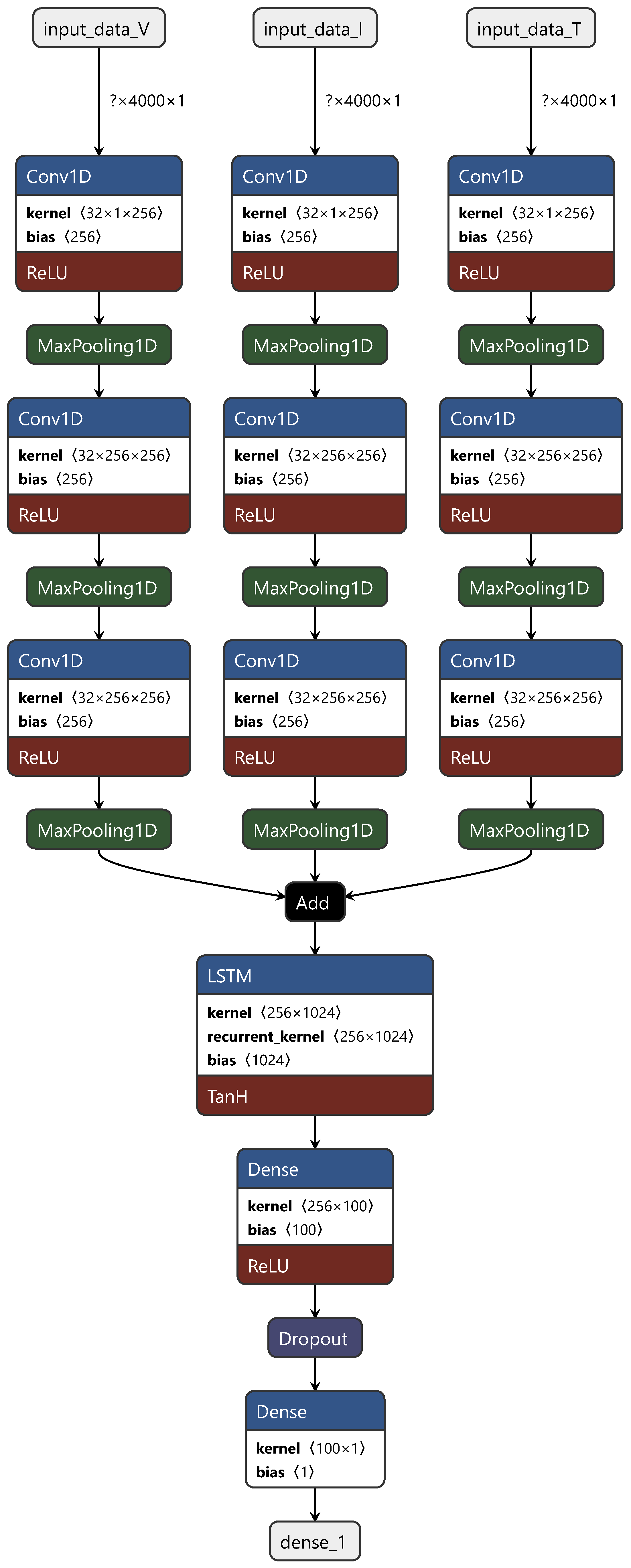
The precise architecture of the proposed model is illustrated in Figure 6.
The inputs of the model include the battery temperature with a size of 4000 × 1 denoted as input_data_T, the battery voltage with size 4000 × 1 represented as input_data_V, and the battery current with size 4000 × 1 denoted as input_data_I. The desired output of the model is the battery capacity, which is a scalar value with size 1 × 1 .

3. Model Deployment and Optimization

3.1. Hardware Specifications

The Jetson family of devices is widely utilized for hardware acceleration in both academia and industry. Several studies such as [27,28,29,30,31] have employed the Jetson family of devices for model deployment and achieved significant speedups.
All deployments discussed in this paper were carried out on the Jetson Xavier NX, one of the low-power embedded platforms of the NVIDIA Jetson family designed for GPU-accelerated computing. The device specifications can be found in Table 2. The Linux for Tegra (L4 T) operating system, bundled with a custom Compute Unified Device Architecture (CUDA) kernel and software libraries that support programming in C++ or Python, comes along with the NVIDIA Jetson.
For model deployment in this study, we utilized JetPack 5.0.2 and TensorRT 8.4.1. Additionally, we set the power mode to maximum power, which ensures that the computing performance of the device remains unrestricted.

3.2. Model Deployment on FPGA Development Board

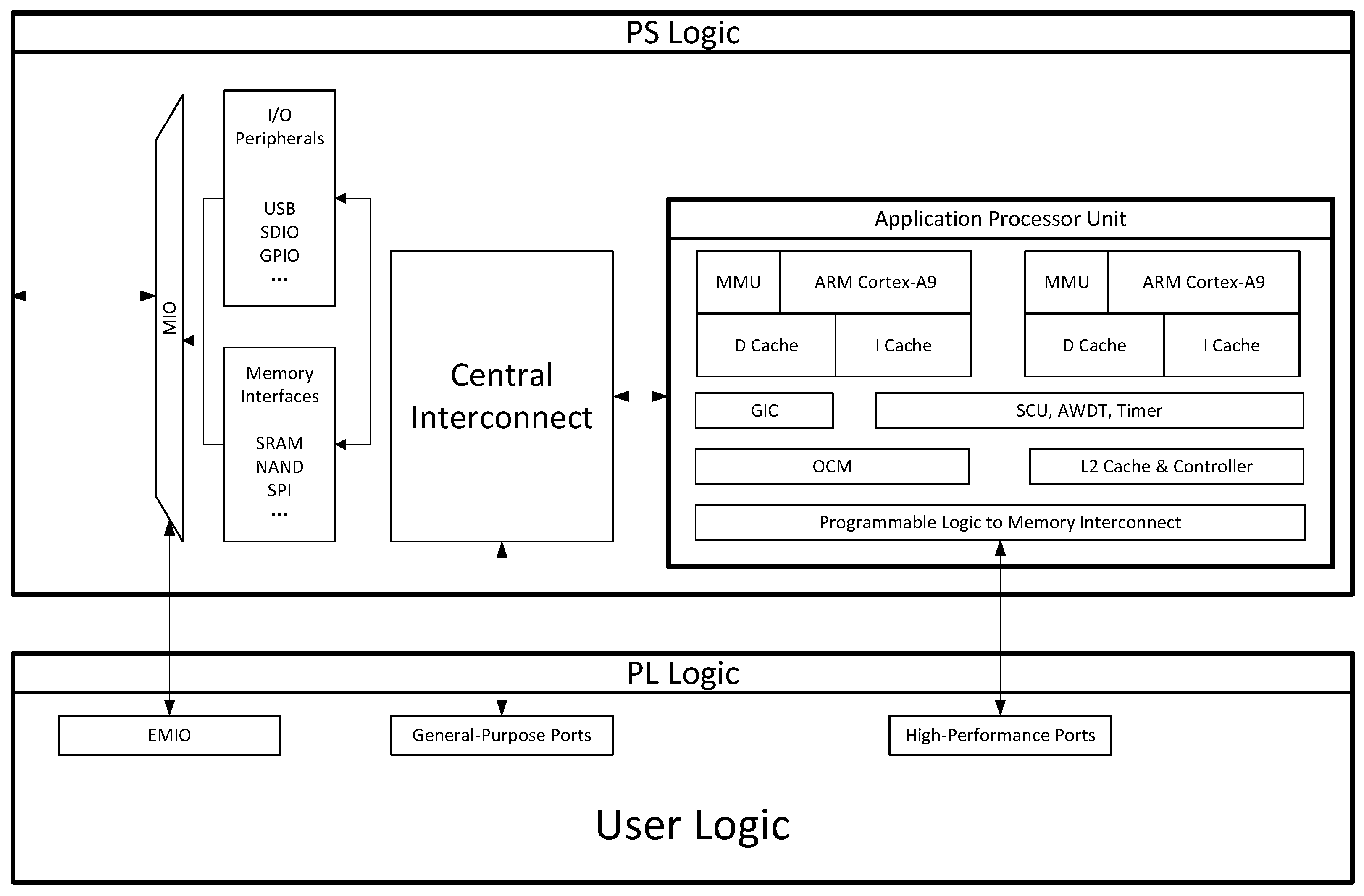
Recent advances in silicon technology have enabled the integration of complex systems onto a single chip. Field Programmable Gate Array (FPGA) devices now consist not only of programmable fabrics, but also hard-core processors, dedicated processing blocks and various peripheral interfaces [32]. The PYNQ-Z1 is an open-source hardware platform that is part of the Xilinx Zynq System-on-Chip (SoC) devices. It offers a unique combination of programmable logic capabilities and processing power, integrating an FPGA with the dual-core ARM Cortex-A9 processor as shown in the functional block diagram of the Xilinx Zynq SoC presented in Figure 7. The PS refers to the dual-core ARM Cortex-A9 processor, while the PL refers to the FPGA fabric. One of the most advantageous features of the PYNQ-Z1 is its Python interface, which allows developers to communicate with PL from Python programs running in the PS. This feature provides a great opportunity for developers who want to implement hardware-accelerated applications like computer vision and machine learning applications. Both academia and industry have seen numerous researchers attempting to accelerate artificial intelligence or image processing operations using the Xilinx Zynq SoC devices. Refs. [33,34,35,36] have deployed various neural networks and achieved impressive optimization results.
To begin working with PYNQ-Z1, we obtained the latest PYNQ image from the Xilinx website and flashed it onto a MicroSD card. After setting up the board, necessary software such as Jupyter Notebook should be installed. Testing data are stored on the MicroSD card and can be accessed through Python scripts, which read the data from the PS and pass it to the PL for processing. Once processing is complete, the data are passed back to the PS from the PL.

3.3. Model Deployment on CPU

Google TensorFlow is a platform for developing machine learning models that can be trained and inferred on various hardware, including CPUs and GPUs. TensorFlow is not only a deep learning framework based on C++, but also an open-source Python API. It is mainly used to build neural networks and can be applied in various fields like target detection, image classification, speech recognition and more. For instance, refs. [37,38] have utilized TensorFlow to deploy Deep Neural Networks (DNNs) for image classification, while refs. [39,40] have successfully applied TensorFlow to implement Recurrent Neural Networks (RNNs) for speech recognition.
The basic unit in TensorFlow is a computational graph, which constructs a queue of nodes with no dependencies to establish the order of computation for the graph. The program conducts the nodes in the queue in a certain order, ensuring fewer unresolved dependencies until the entire graph is computed. TensorFlow is capable of supporting parallelized computation by assigning each node to a device for computation. Furthermore, TensorFlow’s core is implemented in C++, granting it high computing performance. Additionally, TensorFlow is compatible with the CUDA toolkit, allowing users to specify a GPU for computation, which improves efficiency significantly.
The model was previously deployed on the CPU version of TensorFlow. Data are fed into the model one set at a time, and only the inference time is calculated.

3.4. Model Deployment on GPU

The present model is executed using the GPU version of TensorFlow, which employs the interface provided by the CUDA toolkit to execute calls to the GPU. By sending the input data to the GPU for computation, TensorFlow has successfully migrated the inference process, which has significantly decreased the inference time. However, this approach also introduces additional time required for data transfer.
During the model’s testing phase, solely the inference time is computationally relevant, while the data transfer time is not calculated.

3.5. Model Deployment on TensorRT

TensorRT is a software development kit (SDK) designed for fast inference. As shown in Figure 8, the TensorRT workflow involves the creation of an optimized inference engine builder module, which references network definitions. TensorRT is straightforward to deploy and is supported by NVIDIA through their TensorRT API. Unlike the deployment of the GPU version of TensorFlow, TensorRT automatically optimizes network models by merging network structures, allowing for more efficient parallel processing. In addition, TensorRT pre-copies network structures to the GPU to lessen the time required for subsequent inference, although this does result in a longer boot-up time compared to the fast boot-up times of CPU and GPU. Despite this drawback, the inference time of TensorRT is smoother and more stable compared to GPU, especially for the first 3–5 inference processes. The GPU is likely to experience unstable inference latency during this time, resulting in a significantly longer time spent compared to subsequent inference processes. On the other hand, the inference time of TensorRT remains consistent (with no significant difference between the first and subsequent runs).
During testing, time spent on data transfer is not counted, and only the inference time is evaluated.

3.6. Model Optimization with INT8 Quantization

Model quantization, which is an optimization technique capable of reducing model size and speeding up deep learning inference, has received increasing attention from both academia and industry. Although there is a possibility of reduced accuracy compared to previous models, quantized models have practical advantages such as faster inference, smaller model size, and improved throughput.
Based on different quantization phases, quantization methods can be broadly divided into “Quantization Aware Training” (QAT) and “Post-Training Quantization” (PTQ).
QAT requires the quantization of deviation during the training phase, which results in lower accuracy loss. Researchers such as [41,42,43,44] have reduced the inference deviation of the quantized model by identifying the source of deviation during quantization.
On the other hand, PTQ directly quantifies the commonly trained model, is simple, and does not require quantization in the training phase. Since retraining an existing model is often impractical in production environments, PTQ is usually preferred. Despite being less accurate than QAT, PTQ demonstrated equal inference speed in studies conducted by [45,46,47,48].
TensorRT utilizes the PTQ method for quantization, as illustrated in Figure 9. TensorRT offers “calibration”, a technique that measures the activation distribution within each activation tensor as the network performs on input data. It then utilizes that distribution to estimate the tensor’s scale value. By only providing input data, TensorRT can automatically run the network and gather statistical information on each activation tensor, allowing for better accuracy of the quantized model. The calibration process requires just a small number of representative samples, making it highly feasible in practice.
We employed the TensorRT API provided by NVIDIA to perform model quantization and deployment. Then, we randomly selected 40% of the training set for the TensorRT calibration process.
During testing, only the inference time is calculated, without calculating the data transfer time, as discussed in the previous sections.

4. Experimental Design and Test Results

4.1. Prediction Deviation Test

4.1.1. Mean Absolute Deviation Metrics

In this paper, we evaluate the accuracy of model prediction results by adopting the Mean Absolute Error (MAE) and Mean Absolute Percentage Error (MAPE) metrics.
MAE is calculated using the following equation:
M A E = 1 n i = 1 n | y i ^ y i |
Here, y i ^ represents the predicted result, and y i represents the true value. The range of MAE is [ 0 , + ) . A value of 0 indicates that the prediction result is exactly the same as the true value, while a larger deviation between the predicted results and true values leads to a larger value.
On the other hand, MAPE is calculated using the following equation:
M A P E = 100 % × 1 n i = 1 n | y i ^ y i y i |
Similar to MAE, small values represent better fits in MAPE. The range of MAPE is also [ 0 , + ) , and when it is equal to 0%, it indicates a perfect model fit.
MAPE is particularly suitable for deviation comparison when the values are small. Our evaluation method provides a standardized way to measure accuracy and is essential for the development and optimization of prediction models.

4.1.2. Experiment on Validation Set

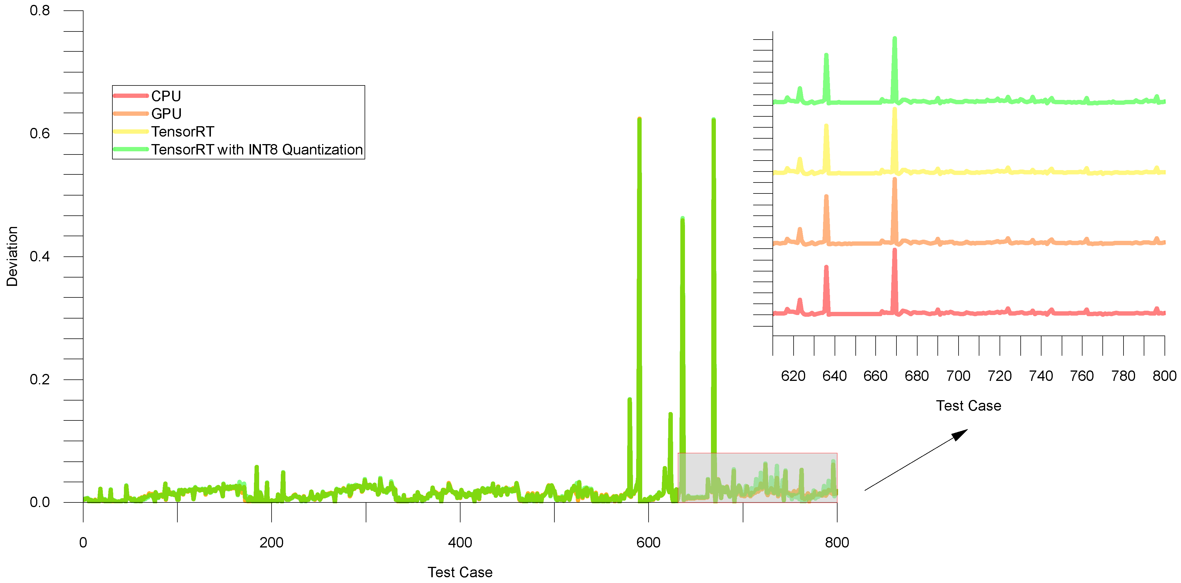
Figure 10 illustrates the deviation between the true and predicted values on the validation set. Meanwhile, Table 3 summarizes the average mean absolute error (MAE) and mean absolute percentage error (MAPE) values for different types, including PYNQ-Z1, CPU, GPU, TensorRT, and TensorRT with INT8. It can be observed that TensorRT did not affect the accuracy, while TensorRT with INT8 had a slight impact on the accuracy.

4.1.3. Experiment on Testing Set

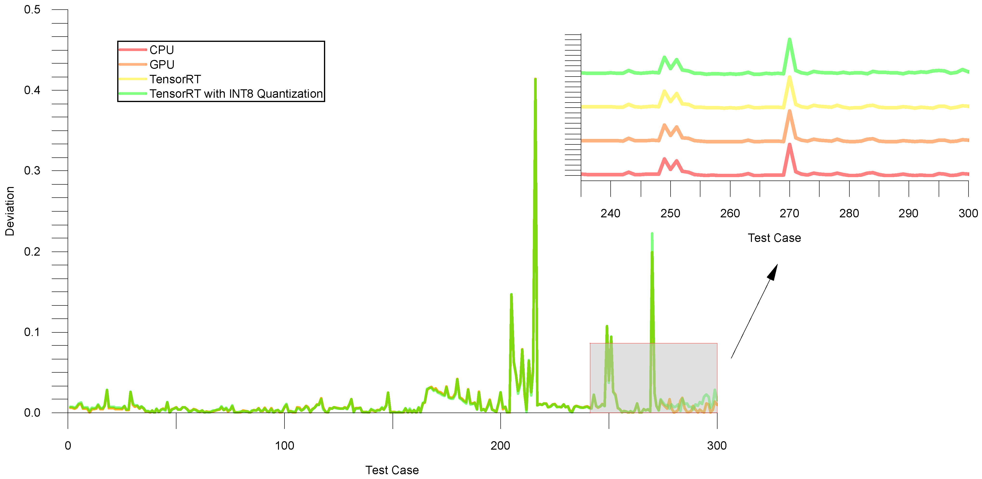
The performance of the model on the testing set is presented in Figure 11, while Table 4 summarizes the average Mean Absolute Error (MAE) values and Mean Absolute Percentage Error (MAPE) values for each approach. The table compares the performance of PYNQ-Z1, CPU, GPU, TensorRT, and TensorRT with INT8 quantization. These findings suggest that utilizing different approaches for accelerating and optimizing performance had a minimal impact on the accuracy of the model.

4.2. Inference Latency Test

4.2.1. Experiment on Validation Set

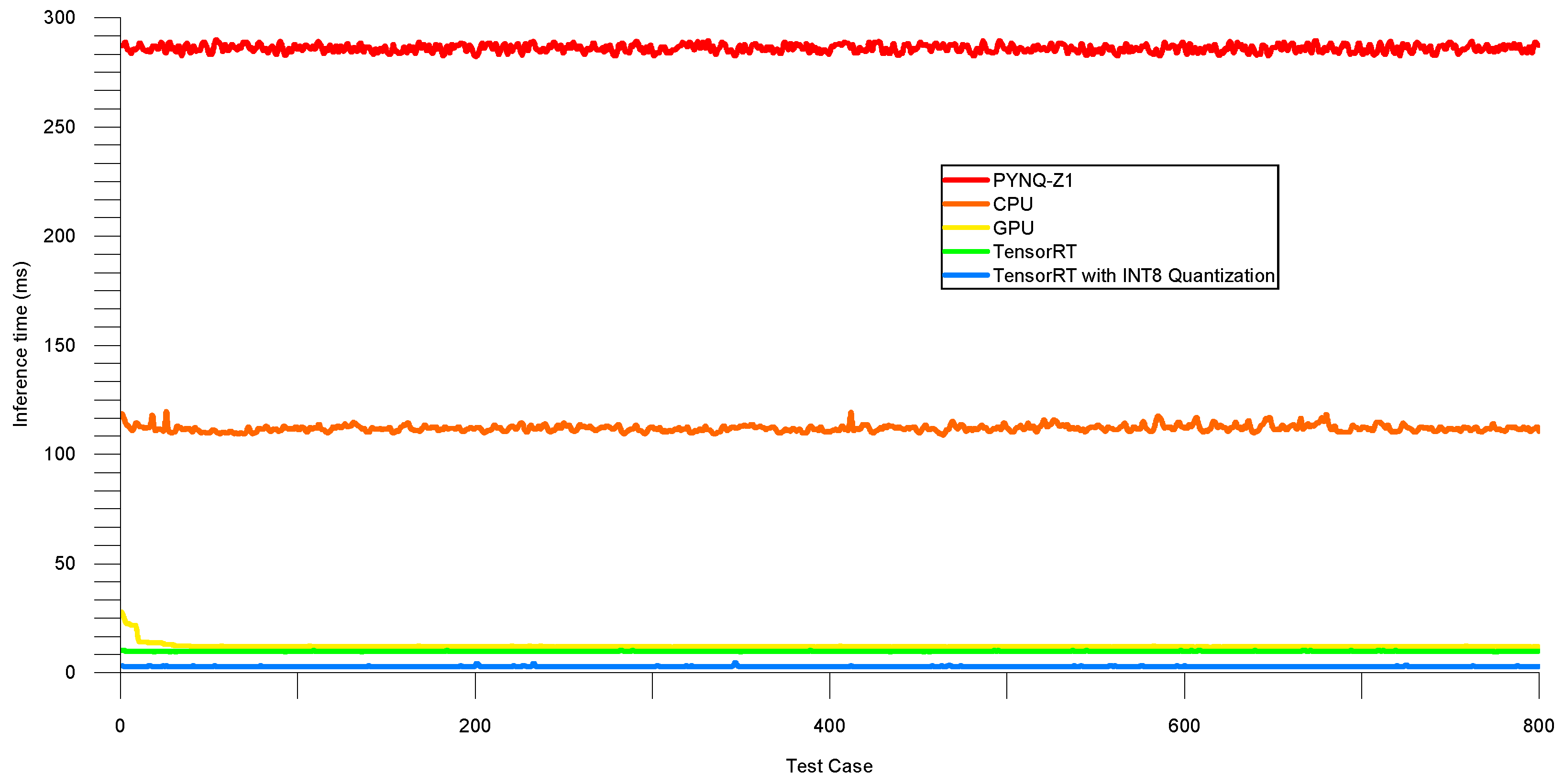
The validation set’s inference time is shown in Figure 12, while Table 5 summarizes the average and median inference latency across different approaches. The table compares the performance of PYNQ-Z1, CPU, GPU, TensorRT, and TensorRT with INT8. The results indicate that TensorRT with INT8 achieved the lowest inference time, with an average latency of 2.897 ms and a median latency of 2.874 ms, followed by TensorRT with an average latency of 9.807 ms and a median latency of 9.791 ms. These results demonstrate the effectiveness of using TensorRT with INT8 quantization for optimizing the model’s performance and achieving low inference latency.

4.2.2. Experiment on Testing Set

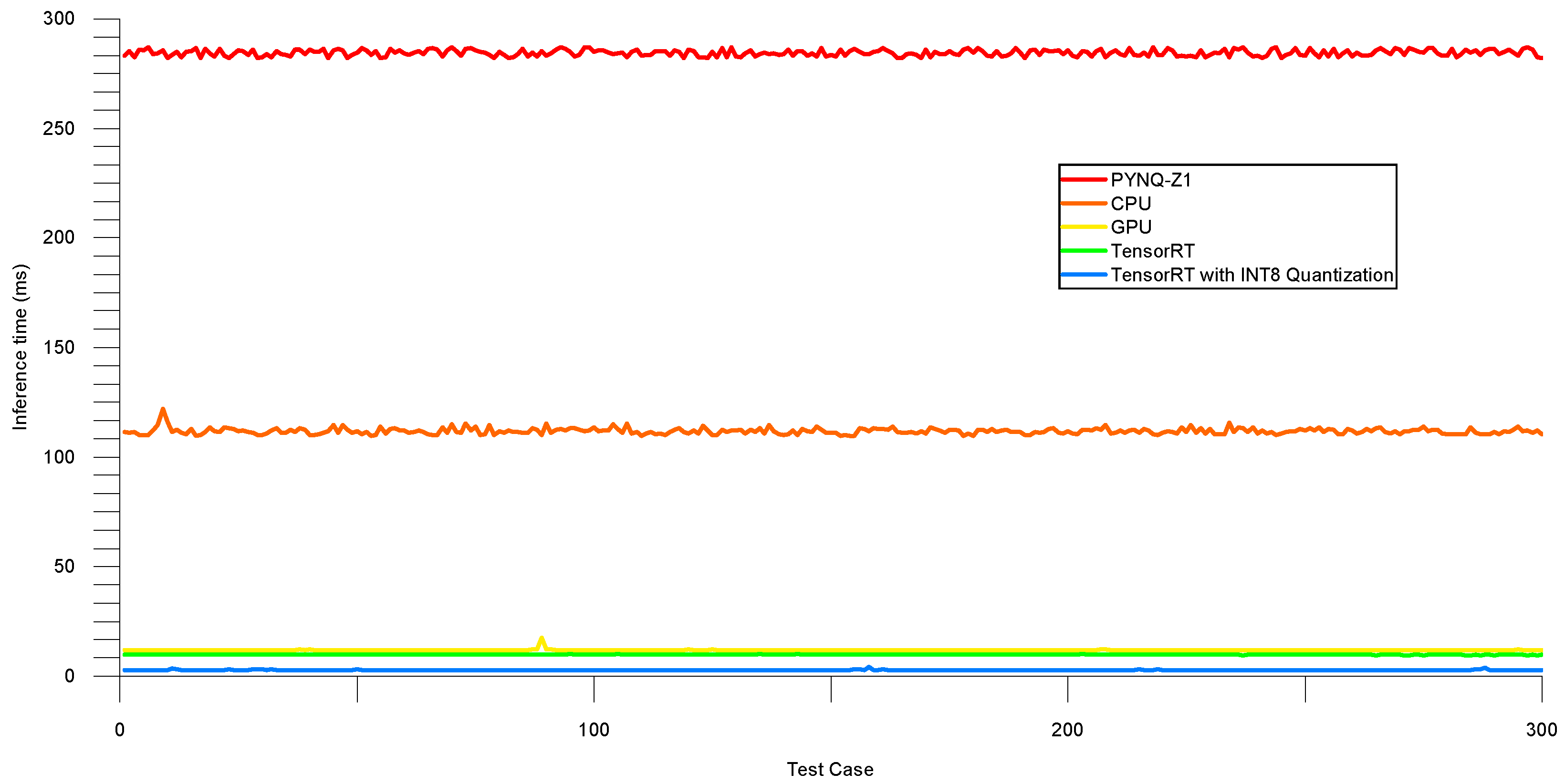
Figure 13 shows the inference time on the testing set. Meanwhile, Table 6 summarizes the average and median inference latency values for different types, including PYNQ-Z1, CPU, GPU, TensorRT, and TensorRT with INT8. The results show that the average and median inference time decrease significantly when using TensorRT and TensorRT with INT8 compared to other devices. Specifically, the median inference latency of TensorRT with INT8 is only 2.874 ms, which is much lower than the other devices.

5. Future Work and Applications

One of the main directions for the development of the battery capacity prediction model is to expand the model’s predictive abilities by exploring and researching new neural network structures. Further training with more diversified, real-world data, such as different battery types and working conditions, would also enhance the model’s ability to fit into actual scenarios. The influence of external factors such as shape, capacity, electrode materials and so on also needs to be explored and incorporated into the training data set. By taking these steps, the model will consider more parameters, which will improve its predictive capabilities in real-world environmental scenarios. Data are critical to any deep learning model; thus, training on a more diverse and extensive dataset, which enhances the model’s flexibility and generalizability, is essential.
Another crucial direction for the development of the battery capacity prediction model is to investigate methods for the more rapid, accurate, and low-cost prediction of the remaining life of a battery and for identifying an individual battery’s degradation trend. This requires using different deep learning-based networks and acceleration techniques to predict the future degradation path of each battery based on historical capacity data. Ultimately, establishing a deep learning-based inference environment to achieve super-fast and precise battery capacity prediction in future battery management systems is worth exploring.
In summary, the future direction for the battery capacity prediction model involves researching new neural network structures, collecting and processing more diverse and extensive datasets, developing an efficient and low-cost prediction approach, incorporating different data sources, discovering new correlations between various factors, and establishing a battery recycling system. These goals are achievable and can lead to significant progress in the field of battery management systems.

6. Conclusions

The application of deep learning in various industries is expected to expand significantly in the near future. In instances where speed is prioritized over accuracy, the inference time of deep learning models becomes a critical factor in determining their popularity in industrial production environments. In this context, there have been limited studies on optimizing and accelerating LSTM networks using multiple techniques to enable the estimation of remaining battery capacity with precision at high speeds on embedded devices.
This work compares the performance of the same models with different optimization and deployment techniques in terms of inference elapsed time and prediction deviation. Through the implementation of TensorRT and quantization techniques, we were able to achieve a significant reduction in inference time from 111 ms to 2 ms, with only a 0.2% increase in MAPE. This achievement will enhance the deployment of high-accuracy models in time-sensitive scenarios and devices, attaining optimized models that are roughly 50× faster than existing models without sacrificing accuracy. Thus, this study is a significant contribution to the use of deep learning models in industry to achieve faster and more precise estimations, which are critical in optimizing production processes.
In the future, various optimization techniques can be employed to reduce the computational cost of inference and improve the real-time performance of deep learning models. Low inference time and high accuracy of deep learning models could enable the application of artificial intelligence in scenarios that require real-time, highly accurate, and low-cost recognition, classification, and prediction, thus opening up numerous possibilities. With continuous research and optimization, it is anticipated that the practicality of deep learning models in today’s industry will expand, leading to further optimizations in various fields.

Author Contributions

Conceptualization, C.Z.; methodology and validation, J.Q.; resources, C.Z.; writing—original draft preparation, J.Q.; writing—review and editing, C.Z.; project administration, C.Z.; funding acquisition, M.G. All authors have read and agreed to the published version of the manuscript.

Funding

This work was supported by the Central Guiding Local Science and Technology Development Fund Projects of China under Grant 2023ZY1008 and Zhejiang Provincial Higher Education “14th Five-Year Plan” Teaching Reform Project (jg20220284).

Institutional Review Board Statement

Not applicable.

Informed Consent Statement

Not applicable.

Data Availability Statement

The original contributions presented in this study are included in the article; further inquiries can be directed to the corresponding author.

Conflicts of Interest

The authors declare no conflicts of interest. The funders had no role in the design of the study; in the collection, analyses, or interpretation of data; in the writing of the manuscript; or in the decision to publish the results.

References

  1. Manthiram, A. An outlook on lithium ion battery technology. ACS Cent. Sci. 2017, 3, 1063–1069. [Google Scholar] [CrossRef]
  2. Wang, Y.; Liu, B.; Li, Q.; Cartmell, S.; Ferrara, S.; Deng, Z.D.; Xiao, J. Lithium and lithium ion batteries for applications in microelectronic devices: A review. J. Power Sources 2015, 286, 330–345. [Google Scholar] [CrossRef]
  3. Masias, A.; Marcicki, J.; Paxton, W.A. Opportunities and challenges of lithium ion batteries in automotive applications. ACS Energy Lett. 2021, 6, 621–630. [Google Scholar] [CrossRef]
  4. Han, X.; Lu, L.; Zheng, Y.; Feng, X.; Li, Z.; Li, J.; Ouyang, M. A review on the key issues of the lithium ion battery degradation among the whole life cycle. ETransportation 2019, 1, 100005. [Google Scholar] [CrossRef]
  5. Li, L.L.; Liu, Z.F.; Tseng, M.L.; Chiu, A.S. Enhancing the Lithium-ion battery life predictability using a hybrid method. Appl. Soft Comput. 2019, 74, 110–121. [Google Scholar] [CrossRef]
  6. Li, Y.; Liu, K.; Foley, A.M.; Zülke, A.; Berecibar, M.; Nanini-Maury, E.; Van Mierlo, J.; Hoster, H.E. Data-driven health estimation and lifetime prediction of lithium-ion batteries: A review. Renew. Sustain. Energy Rev. 2019, 113, 109254. [Google Scholar] [CrossRef]
  7. Xu, F.; Yang, F.; Fei, Z.; Huang, Z.; Tsui, K.L. Life prediction of lithium-ion batteries based on stacked denoising autoencoders. Reliab. Eng. Syst. Saf. 2021, 208, 107396. [Google Scholar] [CrossRef]
  8. Li, W.; Sengupta, N.; Dechent, P.; Howey, D.; Annaswamy, A.; Sauer, D.U. Online capacity estimation of lithium-ion batteries with deep long short-term memory networks. J. Power Sources 2020, 482, 228863. [Google Scholar] [CrossRef]
  9. Graves, A.; Fernández, S.; Schmidhuber, J. Bidirectional LSTM networks for improved phoneme classification and recognition. In Proceedings of the International Conference on Artificial Neural Networks, Munich, Germany, 17–19 September 2005; Springer: Berlin/Heidelberg, Germany, 2005; pp. 799–804. [Google Scholar]
  10. Kim, T.Y.; Cho, S.B. Predicting residential energy consumption using CNN-LSTM neural networks. Energy 2019, 182, 72–81. [Google Scholar] [CrossRef]
  11. Islam, Z.; Abdel-Aty, M.; Mahmoud, N. Using CNN-LSTM to predict signal phasing and timing aided by High-Resolution detector data. Transp. Res. Part C Emerg. Technol. 2022, 141, 103742. [Google Scholar] [CrossRef]
  12. Yao, W.; Huang, P.; Jia, Z. Multidimensional LSTM networks to predict wind speed. In Proceedings of the IEEE 2018 37th Chinese Control Conference (CCC), Wuhan, China, 25–27 July 2018; pp. 7493–7497. [Google Scholar]
  13. Jeong, E.; Kim, J.; Tan, S.; Lee, J.; Ha, S. Deep learning inference parallelization on heterogeneous processors with tensorrt. IEEE Embed. Syst. Lett. 2021, 14, 15–18. [Google Scholar] [CrossRef]
  14. Saurav, S.; Gidde, P.; Saini, R.; Singh, S. Dual integrated convolutional neural network for real-time facial expression recognition in the wild. Vis. Comput. 2022, 38, 1083–1096. [Google Scholar] [CrossRef]
  15. Dai, B.; Li, C.; Lin, T.; Wang, Y.; Gong, D.; Ji, X.; Zhu, B. Field robot environment sensing technology based on TensorRT. In Proceedings of the International Conference on Intelligent Robotics and Applications, Yantai, China, 22–25 October 2021; Springer: Berlin/Heidelberg, Germany, 2021; pp. 370–377. [Google Scholar]
  16. Zhang, Y.; Xiong, R.; He, H.; Pecht, M.G. Long short-term memory recurrent neural network for remaining useful life prediction of lithium-ion batteries. IEEE Trans. Veh. Technol. 2018, 67, 5695–5705. [Google Scholar] [CrossRef]
  17. Park, K.; Choi, Y.; Choi, W.J.; Ryu, H.Y.; Kim, H. LSTM-based battery remaining useful life prediction with multi-channel charging profiles. IEEE Access 2020, 8, 20786–20798. [Google Scholar] [CrossRef]
  18. Zhang, Y.; Xiong, R.; He, H.; Liu, Z. A LSTM-RNN method for the lithuim-ion battery remaining useful life prediction. In Proceedings of the IEEE 2017 Prognostics and System Health Management Conference (PHM-Harbin), Yantai, China, 22–25 October 2017; pp. 1–4. [Google Scholar]
  19. Choi, D.; Lee, D.; Lee, J.; Son, S.; Kim, M.; Jang, J.W. A Study on the Efficiency of Deep Learning on Embedded Boards. J. Converg. Cult. Technol. 2021, 7, 668–673. [Google Scholar]
  20. Jeong, E.; Kim, J.; Ha, S. TensorRT-Based Framework and Optimization Methodology for Deep Learning Inference on Jetson Boards. ACM Trans. Embed. Comput. Syst. 2022, 21, 1–26. [Google Scholar] [CrossRef]
  21. Yang, S.; Niu, Z.; Cheng, J.; Feng, S.; Li, P. Face recognition speed optimization method for embedded environment. In Proceedings of the IEEE 2020 International Workshop on Electronic Communication and Artificial Intelligence (IWECAI), Shanghai, China, 12–14 June 2020; pp. 147–153. [Google Scholar]
  22. Bachtiar, Y.; Adiono, T. Convolutional neural network and maxpooling architecture on Zynq SoC FPGA. In Proceedings of the IEEE 2019 International Symposium on Electronics and Smart Devices (ISESD), Badung-Bali, Indonesia, 8–9 October 2019; pp. 1–5. [Google Scholar]
  23. Li, X.; Yin, Z.; Xu, F.; Zhang, F.; Xu, G. Design and implementation of neural network computing framework on Zynq SoC embedded platform. Procedia Comput. Sci. 2021, 183, 512–518. [Google Scholar] [CrossRef]
  24. Lee, H.S.; Jeon, J.W. Accelerating deep neural networks using FPGAs and ZYNQ. In Proceedings of the 2021 IEEE Region 10 Symposium (TENSYMP), Jeju, Republic of Korea, 23–25 August 2021; pp. 1–4. [Google Scholar]
  25. Lv, H.; Zhang, S.; Liu, X.; Liu, S.; Liu, Y.; Han, W.; Xu, S. Research on dynamic reconfiguration technology of neural network accelerator based on Zynq. J. Phys. Conf. Ser. IOP Publ. 2020, 1650, 032093. [Google Scholar] [CrossRef]
  26. Saha, B.; Goebel, K. Battery Data Set, NASA Ames Prognostics Data Repository; NASA Ames Research Center: Moffett Field, CA, USA, 2007. [Google Scholar]
  27. Mittal, S. A Survey on optimized implementation of deep learning models on the NVIDIA Jetson platform. J. Syst. Archit. 2019, 97, 428–442. [Google Scholar] [CrossRef]
  28. Cui, H.; Dahnoun, N. Real-time stereo vision implementation on Nvidia Jetson TX2. In Proceedings of the IEEE 2019 8th Mediterranean Conference on Embedded Computing (MECO), Budva, Montenegro, 10–14 June 2019; pp. 1–5. [Google Scholar]
  29. Jose, E.; Greeshma, M.; Haridas, M.T.; Supriya, M. Face recognition based surveillance system using facenet and mtcnn on jetson tx2. In Proceedings of the IEEE 2019 5th International Conference on Advanced Computing & Communication Systems (ICACCS), Coimbatore, India, 15–16 March 2019; pp. 608–613. [Google Scholar]
  30. Bokovoy, A.; Muravyev, K.; Yakovlev, K. Real-time vision-based depth reconstruction with nvidia jetson. In Proceedings of the IEEE 2019 European Conference on Mobile Robots (ECMR), Prague, Czech Republic, 4–6 September 2019; pp. 1–6. [Google Scholar]
  31. Süzen, A.A.; Duman, B.; Şen, B. Benchmark analysis of jetson tx2, jetson nano and raspberry pi using deep-cnn. In Proceedings of the IEEE 2020 International Congress on Human-Computer Interaction, Optimization and Robotic Applications (HORA), Ankara, Turkey, 26–27 June 2020; pp. 1–5. [Google Scholar]
  32. Tambara, L.A.; Kastensmidt, F.L.; Medina, N.H.; Added, N.; Aguiar, V.A.; Aguirre, F.; Macchione, E.L.; Silveira, M.A. Heavy ions induced single event upsets testing of the 28 nm Xilinx Zynq-7000 all programmable SoC. In Proceedings of the 2015 IEEE Radiation Effects Data Workshop (REDW), New Orleans, LA, USA, 17–21 July 2015; pp. 1–6. [Google Scholar]
  33. Sharma, A.; Singh, V.; Rani, A. Implementation of CNN on Zynq based FPGA for real-time object detection. In Proceedings of the IEEE 2019 10th International Conference on Computing, Communication and Networking Technologies (ICCCNT), Kanpur, India, 6–8 July 2019; pp. 1–7. [Google Scholar]
  34. Wang, E.; Davis, J.J.; Cheung, P.Y. A PYNQ-based framework for rapid CNN prototyping. In Proceedings of the 2018 IEEE 26th Annual International Symposium on Field-Programmable Custom Computing Machines (FCCM), Boulder, CO, USA, 29 April–1 May 2018; p. 223. [Google Scholar]
  35. Viet Huynh, T. FPGA-based acceleration for convolutional neural networks on PYNQ-Z2. Int. J. Comput. Digit. Syst. 2021, 11, 441–449. [Google Scholar] [CrossRef] [PubMed]
  36. Sun, S.; Zou, J.; Zou, Z.; Wang, S. Neural network experiment on PYNQ. In Experience of PYNQ: Tutorials for PYNQ-Z2; Springer: Berlin/Heidelberg, Germany, 2023; pp. 45–79. [Google Scholar]
  37. Abu, M.A.; Indra, N.H.; Rahman, A.; Sapiee, N.A.; Ahmad, I. A study on Image Classification based on Deep Learning and Tensorflow. Int. J. Eng. Res. Technol. 2019, 12, 563–569. [Google Scholar]
  38. Kothari, J.D. A case study of image classification based on deep learning using TensorFlow. Int. J. Innov. Res. Comput. Commun. Eng. 2018, 6, 3888–3892. [Google Scholar]
  39. Escur i Gelabert, J. Exploring Automatic Speech Recognition with TensorFlow. Bachelor’s Thesis, Universitat Politècnica de Catalunya, Barselona, Spain, 2018. [Google Scholar]
  40. Medvedev, M.; Okuntsev, Y. Using Google tensorFlow machine learning library for speech recognition. J. Phys. Conf. Ser. C IOP Publ. 2019, 1399, 033033. [Google Scholar] [CrossRef]
  41. Shen, M.; Liang, F.; Gong, R.; Li, Y.; Li, C.; Lin, C.; Yu, F.; Yan, J.; Ouyang, W. Once quantization-aware training: High performance extremely low-bit architecture search. In Proceedings of the IEEE/CVF International Conference on Computer Vision, Montreal, BC, Canada, 11–17 October 2021; pp. 5340–5349. [Google Scholar]
  42. Mishchenko, Y.; Goren, Y.; Sun, M.; Beauchene, C.; Matsoukas, S.; Rybakov, O.; Vitaladevuni, S.N.P. Low-bit quantization and quantization-aware training for small-footprint keyword spotting. In Proceedings of the 2019 18th IEEE International Conference On Machine Learning And Applications (ICMLA), Boca Raton, FL, USA, 16–19 December 2019; pp. 706–711. [Google Scholar]
  43. Park, E.; Yoo, S.; Vajda, P. Value-aware quantization for training and inference of neural networks. In Proceedings of the European Conference on Computer Vision (ECCV), Munich, Germany, 8–14 September 2018; pp. 580–595. [Google Scholar]
  44. Nguyen, H.D.; Alexandridis, A.; Mouchtaris, A. Quantization aware training with absolute-cosine regularization for automatic speech recognition. In Proceedings of the Interspeech, Shanghai, China, 25–29 October 2020; pp. 3366–3370. [Google Scholar]
  45. Nagel, M.; Amjad, R.A.; Van Baalen, M.; Louizos, C.; Blankevoort, T. Up or down? Adaptive rounding for post-training quantization. In Proceedings of the International Conference on Machine Learning. PMLR, Virtual, 13–18 July 2020; pp. 7197–7206. [Google Scholar]
  46. Fang, J.; Shafiee, A.; Abdel-Aziz, H.; Thorsley, D.; Georgiadis, G.; Hassoun, J.H. Post-training piecewise linear quantization for deep neural networks. In Proceedings of the European Conference on Computer Vision, Glasgow, UK, 23–28 August 2020; Springer: Berlin/Heidelberg, Germany; pp. 69–86. [Google Scholar]
  47. Yuan, Z.; Xue, C.; Chen, Y.; Wu, Q.; Sun, G. PTQ4ViT: Post-training quantization for vision transformers with twin uniform quantization. In Proceedings of the European Conference on Computer Vision, Tel Aviv, Israel, 23 October 2022; Springer: Berlin/Heidelberg, Germany, 2022; pp. 191–207. [Google Scholar]
  48. Liu, X.; Ye, M.; Zhou, D.; Liu, Q. Post-training quantization with multiple points: Mixed precision without mixed precision. In Proceedings of the AAAI Conference on Artificial Intelligence 10, San Jose, CA, USA, 12–16 July 2021; Volume 35, pp. 8697–8705. [Google Scholar]
Figure 1. Overview of the dataset.
Energies 17 02797 g001
Figure 2. Charts of battery #5 with aging process. (a) Charging voltage curve; (b) Charging current curve; (c) Charging temperature curve; (d) Capacity degradation curve.
Energies 17 02797 g002
Figure 3. Voltage vs. current curve during battery charging.
Energies 17 02797 g003
Figure 4. LSTM network. (a) The detailed structure within LSTM network; (b) LSTM transmission line.
Energies 17 02797 g004
Figure 5. 3 types of gates. (a) Forget gate; (b) Input gate; (c) Output gate.
Energies 17 02797 g005
Figure 6. Model network structure.
Energies 17 02797 g006
Figure 7. Block diagram of Xilinx Zynq SoC.
Energies 17 02797 g007
Figure 8. TensorRT workflow.
Energies 17 02797 g008
Figure 9. TensorRT with INT8 Quantization workflow.
Energies 17 02797 g009
Figure 10. The deviation between the true value and the predicted value (validation set).
Energies 17 02797 g010
Figure 11. The deviation between the true value and the predicted value (testing set).
Energies 17 02797 g011
Figure 12. Inference time (validation set).
Energies 17 02797 g012
Figure 13. Inference time (testing set).
Energies 17 02797 g013
Table 1. Battery specifications sourced from [26].
No.ChargingDischargingOperating ConditionsDataset
CC a (A)UV b (V)CoC c (mA)CC (A)CoV d (V)OT e (°C)IC f (Ah)EC g (Ah)
#51.54.22022.7241.861.32Training
#61.54.22022.5242.041.18
#181.54.22022.5241.861.34
#291.54.22042431.841.61
#301.54.22042.2431.781.56
#311.54.22042.5431.831.66
#391.54.22022.524, 440.471.31
#401.54.22042.724, 440.790.55
#461.54.22012.241.721.15
#471.54.22012.541.671.15
#481.54.22012.741.661.22
#71.54.22022.2241.891.43Validation
#321.54.22042.7431.891.63
#381.54.22012.224, 441.11.53
#461.54.22012.241.721.15Testing
a CC represents constant current, b UV represents upper voltage, c CoC represents cut-off current, d CoV represents cut-off voltage, e OT represents operating temperature, f IC represents initial capacity, g EC represents end capacity.
Table 2. Jetson Xavier NX specifications.
TypeSpecification
GPU384-core NVIDIA Volta™
CPU6-core NVIDIA Carmel ARM®
Memory8 GB 128-bit LPDDR4x
Storage64 GB Sandisk microSD card
AI Performance21 TOPS
Table 3. MAE and MAPE on validation set.
TypeMAEMAPE
PYNQ-Z10.016242.77%
CPU0.016242.77%
GPU0.016242.77%
TensorRT0.016242.77%
TensorRT with INT80.016692.84%
Table 4. MAE and MAPE on testing set.
TypeMAEMAPE
PYNQ-Z10.011841.47%
CPU0.011841.47%
GPU0.011841.47%
TensorRT0.011841.47%
TensorRT with INT80.012831.62%
Table 5. Inference latency on validation set.
TypeAverage (ms)Median (ms)
PYNQ-Z1285.943285.956
CPU111.975111.754
GPU18.83511.869
TensorRT9.8079.791
TensorRT with INT82.8972.874
Table 6. Inference latency on testing set.
TypeAverage (ms)Median (ms)
PYNQ-Z1284.531284.631
CPU111.740111.579
GPU11.90511.873
TensorRT9.7729.754
TensorRT with INT82.8952.874
Disclaimer/Publisher’s Note: The statements, opinions and data contained in all publications are solely those of the individual author(s) and contributor(s) and not of MDPI and/or the editor(s). MDPI and/or the editor(s) disclaim responsibility for any injury to people or property resulting from any ideas, methods, instructions or products referred to in the content.