Abstract
Recent advances in high-power applications employing voltage source converters have been primarily fuelled by the emergence of the modular multilevel converter (MMC) and its derivatives. Model predictive control (MPC) has emerged as an effective way of controlling these converters because of its high response. However, the practical implementation of MPC encounters hurdles, particularly in MMCs featuring many sub-modules per arm. This research introduces an approach termed folding model predictive control (FMPC), coupled with a pre-processing sorting algorithm, tailored for modular multilevel converters. The objective is to alleviate a significant part of the computational burden associated with the control of these converters. The FMPC framework combines multiple control objectives, encompassing AC current, DC current, circulating current, arm energy, and leg energy, within a unified cost function. Both simulation studies and real-time hardware-in-the-loop (HIL) testing are conducted to verify the efficacy of the proposed FMPC. The findings underscore the FMPC’s ability to deliver fast response and robust performance under both steady-state and dynamic operating conditions. Moreover, the FMPC adeptly mitigates circulating currents, reduces total harmonic distortion (THD%), and upholds capacitor voltage stability within acceptable thresholds, even in the presence of harmonic distortions in the AC grid. The practical applicability of MMCs, notwithstanding the presence of a large number of sub-modules (SMs) per arm, is facilitated by the significant reduction in switching states and computational overhead achieved through the FMPC approach.
1. Introduction
Modular multilevel converters are now well established and have the capability to combine high modularity and scalability requirements in high-power applications effectively. However, devising a control scheme that addresses multiple control objectives while ensuring optimal functionality of the converter poses significant challenges. Implementing linear controllers within the MMC necessitates the use of numerous cascaded and parallel control loops, resulting in complex control architectures [1]. Linear controllers typically demonstrate complex structures, slow and interdependent dynamic responses, and a limited stable operational range [2]. Additionally, fine-tuning parameters for linear controllers in MMCs is notably challenging, especially when aiming for multi-objective regulation within cascaded or parallel structures [3,4].
On the contrary, model predictive control (MPC) has emerged as a leading choice for controlling MMCs due to its fast dynamic response, simplicity, and ability to handle multiple control objectives within a unified cost function [5,6]. However, a notable drawback arises from the exponential increase in the number of switching states that must be considered at each sampling interval, making the practical implementation of MPC unfeasible. Several noteworthy studies have been conducted to tackle this particular challenge.
The main strategies for implementing MPC in MMC applications revolve around two primary approaches: indirect MPC and modulated MPC. In the first approach, researchers have aimed to address computational complexities by incorporating a sorting algorithm following the MPC process. In this method, the MPC process determines the number of SMs to be integrated into the upper and lower arms, while a capacitor voltage sorting algorithm is simultaneously employed to equalise voltages across the submodules’ capacitors [2,3,7,8,9]. Typically, in the case of a single-phase MMC, the reduction in the number of switching states to is achieved (where N is the number of sub-modules per arm), with further improvements in computational efficiency achieved through the refinement of the sorting technique, as demonstrated in studies [7,8,9].
The modulated MPC approach shares more similarities with the linear proportional integral (PI) method, generating a voltage reference as its output, which can then be implemented using an appropriate modulation technique. This approach combines the MPC system with both the sorting algorithm technique and one of the modulation techniques [10,11,12,13,14,15,16]. Here, the role of MPC is to predict the voltage-modulating demand and send this directly to the pulse-width modulation (PWM) elements to produce the required pulses, while the sorting algorithm ensures capacitor balancing. The computational burden linked with the modulated MPC strategy exhibits a linear correlation with the quantity of SMs within the MMC. Nonetheless, its latency in responsiveness is relatively prolonged in contrast to the indirect MPC method [16].
Alternative research efforts have focused on mitigating the computational burden in MPC, either by extending existing strategies or enhancing the MPC algorithm itself.
The hierarchical linear control strategy was implemented in [17]. The MPC part is placed in one of the stages of this hierarchy to enhance the performance of the control system. The authors of [18] cascade two modulated MPC, or as they call it, use a continuous control set MPC (CCS-MPC) to simplify the conventional CCS-MPC approach. A hybrid MPC was implemented in [19] by integration between the conventional finite control set MPC (FCS-MPC) and the modulated MPC. This strategy was updated in [20] by simplifying the search of the horizon using a quadratic program. The computational burden was reduced in [21] by adding an insertion index combinations step to the MPC block, enabling the prediction process to be achieved faster. Further reduction in the switching states of the indirect MPC was proposed in [22] by narrowing the horizon of the predictor search by making it only consider the optimal switching sequence.
In [23], the researchers proposed a method to reduce the number of switching states by dividing the SMs per arm into M subgroups and employing a sorting technique twice. The initial sorting determines the number of subgroups to be inserted from each arm. Subsequently, the second sorting occurs within the last subgroup, consisting of X SMs each, to specify the particular SMs for insertion. If applied separately to each arm in a 3-phase system, this method reduces the number of switching states to .
The proposed sequential phase-shifted MPC (PS-MPC) method for the MMC utilises the operational principle of the well-known phase-shifted PWM (PS-PWM). This method effectively obtains independent modulating signals for each carrier in a sequential manner [1].
Deadbeat predictive current control, a model-based control technique, was previously employed in the control of MMC systems [4]. This approach provides a fast dynamic response similar to traditional MPC but with a notably decreased computational burden. This is accomplished by directly calculating the optimal voltage references without requiring switching state evaluation, cost function computation, or weighting factor selection.
In [24], a simplified optimisation algorithm is presented, operating within the scope of () optimisations. In subsequent work [2], computational complexity was further reduced by limiting the optimisation scope of each bridge arm, albeit resulting in a decrease in the number of output voltage levels. When implementing the described MPC method, the total number of output voltage levels achieved is (). In contrast to a control approach yielding an output voltage level count of (), this algorithm fails to mitigate low-frequency harmonics within the circulating current, thereby resulting in higher THD in the output current [25].
In [25], a compensatory model predictive current control (CMPCC) method is developed to improve control effectiveness while reducing computational complexity. Unlike traditional MPC, this algorithm succeeds in reducing the computational burden while maintaining the output voltage at ().
A fast finite level state MPC (FFS-MPC) is presented in [26]. The authors substituted the cost function optimisation step (iteration step) by solving a system of linear equations, which represent the control objectives of the MMC.
The proposal outlined in [27] integrates model-free adaptive control (MF-AC), employing a data-driven strategy, with a model-based control method rooted in MPC. This integration relies solely on the input-output measurement data of the MPC controller, without depending on expert knowledge of explicit models or system parameters. This fusion leads to an architecture termed data-driven-based predictive current control (DD-PCC). Leveraging artificial intelligence to emulate MPC can effectively alleviate computational demands. In [28,29], a machine learning approach grounded in MPC is introduced, where a neural network is trained using datasets derived from the model of MPC methodology. This approach enables the neural network to mimic MPC functionality based on the information acquired from the datasets of the MPC model. In [30], an event-triggered mechanism is integrated with an MPC-based neural network.
In light of the multifaceted challenges encountered in the control systems of MMCs, the pursuit of a robust control strategy capable of simultaneously addressing various control objectives and constraints remains paramount. The techniques outlined above highlight the complexities inherent in MMC, each necessitating certain concessions in their implementation. For instance, while indirect MPC methods rely on averaged capacitor voltages for optimisation, they introduce errors in prediction. Similarly, the modulated MPC exhibits a longer dynamic response compared to conventional MPC methods. Moreover, strategies aimed at reducing the number of switching states often result in heightened control system complexity, thereby exacerbating the computational burdens.
In response to these challenges, the proposed FMPC paradigm represents a promising advancement. By leveraging actual capacitor voltage values for prediction, FMPC overcomes the inaccuracies associated with averaged voltages, thus embodying the principles of direct MPC. This ensures a rapid dynamic response while accommodating multiple control objectives within a unified cost function. Crucially, FMPC achieves a reduction in both the switching states and the computational burden without sacrificing predictive accuracy. In essence, FMPC emerges as a streamlined solution capable of optimising MMC performance with heightened efficiency and precision.
Following an introduction to MMC modelling, conventional MPC will be explained, followed by the proposed folding MPC approach. Subsequently, the HIL setup will be outlined, and simulation and HIL results will be presented. Finally, conclusions will be drawn based on the findings from the results.
2. Modelling of MMC
The MMC topology was initially introduced in 2003 [31] and has emerged as a cornerstone in the realm of HVDC applications. Renowned for its modularity and scalability, MMC has played a pivotal role in shaping the landscape of HVDC technology. Notably, the inception of the first point-to-point VSC-HVDC project based on MMC architecture took place in 2010 [32]. Since this groundbreaking milestone, a multitude of VSC-HVDC projects utilising this converter have been successfully implemented worldwide. Table 1 provides an overview of select projects across the globe, showcasing the widespread adoption and impact of this technology. Additionally, further insights into current and forthcoming projects can be found in reference [33], which mentions both present endeavours and future planning initiatives.

Table 1.
Some of the VSC-HVDC projects based on MMCs.
A 3-phase MMC consists of three identical legs, one per phase, where each leg is divided in half at the AC connection to create the upper and lower arms, as illustrated in Figure 1. Each arm comprises N cascaded SMs connected in series with an arm inductor . The incorporation of arm inductors in the MMC serves to minimise circulating current induced by voltage disparities between the upper and lower arms, while also reducing the rate of change of the short-circuit current on the DC side [51].
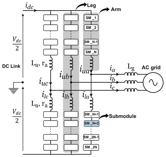
Figure 1.
Topology of MMC.
Typically, each SM comprises a half-bridge power converter connected to a capacitor. The arrangement of capacitance in the SM eliminates the need for a high-voltage DC link capacitor, enabling the generation of high-quality AC voltage, low voltage stress (), low switching frequency, and enhanced efficiency [52].
The upper and lower arm voltages are determined using the total summation of voltages across the inserted SMs at any given moment. As a result, each series of SMs within an arm is replaced with a regulated voltage source characterised by the following values:
where , and are the upper arm voltage, lower arm voltage, upper switching state, lower switching state, upper capacitor voltages, and the lower capacitor voltages, respectively. When Kirchhoff’s voltage law is employed to analyse the upper and lower arms of the single-phase average model, the resultant equations are outlined below:
where , and are the upper, lower, and AC current, respectively, and is the grid voltage. The AC side equivalent circuit of an MMC is represented by Equation (5), which is found by adding Equations (3) and (4).
where
The AC side equivalent circuit comprises two AC voltage sources, an inductor, and a resistor connected in series, as depicted in Equation (7).
where is a terminal AC voltage of the MMC
The DC equivalent circuit can be derived by subtracting Equation (4) from Equation (3), as demonstrated below:
The equivalent DC side circuit contains two DC voltage sources, an inductor, and a resistor connected in series, as represented in Equation (10).
where , is the terminal DC voltage of the MMC, and is the arm’s circulating current.
The total of the upper arm currents must equal the total of the lower arm currents, both of which must also match the DC current. This relationship can be expressed mathematically as follows:
It is important to note that the circulating current exists within each arm and consists of two elements. The first element is the DC component, calculated as (where P denotes the number of phases). The second element is at twice the fundamental frequency of the output current. A primary goal of the control system is to eliminate this second-order component from the circulating current in an effort to diminish the RMS arm currents and subsequently reduce the losses in the converter. Therefore, the objective is to achieve a circulating current that is solely DC in nature.
3. Conventional MPC
In contrast to linear control methods, this approach obviates the requirement for linear PI regulators, voltage sorting of capacitors, and modulation stages. Moreover, it presents a fundamentally distinct strategy for managing power converters. Traditional control techniques intervene only after an error has manifested. Conversely, MPC proactively executes control measures even before significant current errors occur. In order to achieve this, it leverages a discretisation strategy of the mathematical model to predict the converter’s future behaviour. Illustrated in Figure 2, the finite control set MPC (FCS-MPC) comprises an extrapolation of the reference values, the predictive model, and the cost function.
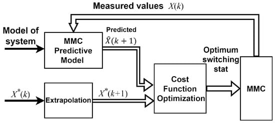
Figure 2.
Block diagram of FCS-MPC for controlling MMC.
- Extrapolation of reference currents from the to the sampling instant;
- Predictive model to calculate future control objectives across all feasible switching states;
- Cost function to evaluate predictions and select optimal gating signals.
As discussed previously, multiple control objectives are included within a single cost function. This paper considers five control objectives: control of the AC current, DC current, circulating current, energy per arm, and energy per leg. The MPC is integrated into the digital controller in discrete form, necessitating the representation of control objectives in the discrete time domain. Subsequently, for the remainder of this section, all the aforementioned control objectives will be discretised accordingly. To convert the continuous model into a discrete model, the forward Euler approximation discretisation method is commonly employed due to its simplicity and practicality [53]. This method enables the prediction of a future step at () based on the present state at (k), aligning with the fundamental principle of MPC. The forward Euler approach approximates the derivative as follows:
The primary control objective is the AC current, which holds significant importance in MMC applications. The dynamic model of the output current can be derived from Equation (7), and the discrete-time model of the AC current is expressed as follows:
The second control objective is a DC current which is divided identically into 3-phase arm currents. If Equation (9) is applied to phase a, b, and c, respectively, then the dynamic model of the DC current can be found from Equation (13), as shown below:
The discrete time model of the DC current will be:
Then, the dynamic model of the circulating currents can be obtained from Equation (10). So that the discrete form of the circulating current is:
Ultimately, the energies of both arms and legs must be discretised. During the design phase, the capacitor voltage of each SM is determined as . Consequently, to guarantee energy balance, the sum of all the capacitor voltages (both inserted and bypassed) per arm should equal the DC voltage, with a fluctuation tolerance of less than ±10%, i.e.,
This equilibrium results in minimisation of the power losses to their lowest extent, without significant stress induced by voltage imbalances in any particular arm. The energy variation per arm can be mathematically expressed as:
The power or energy variation in Equations (20a) and (20b) can be rewritten in another form depending on the arm current and voltage per arm as follows:
By adding and subtracting the above equations, the following simplification can be obtained:
Based on Equations (6), (8), (11), and (12), the alternative forms of Equations (22) and (23) are as follows:
Energy balancing is attainable when the energy difference, or the value described in Equation (25), equals zero. Additionally, the second balancing requirement among phases necessitates that the average energy be identical in each leg. The desired energy per leg is represented as follows:
Thus, the discrete time model of the arm and phase energies is:
The predictive model utilises all the discretised equations mentioned above to compute future objective values. Given a finite set of switching states, these values can be systematically listed for all viable configurations. In 3-phase MMC systems, the usual number of switching states amounts to .
The predicted control objectives undergo evaluation using a cost function, which is defined as the summation of either the absolute or squared errors between the reference and predicted objectives. The weighting of previous control objectives depends on their respective impacts on the control system. Consequently, there are five weighting factors, denoted as , and , each corresponding to a control objective. The cost function is formulated as shown in Equation (29):
where all asterisked elements in the cost function are reference values, and the absolute error method is dependent on the evaluation of the optimum switching states.
The optimal action, which minimises the error at the subsequent sampling instance, is selected and swiftly executed on the MMC. FCS-MPC delivers a dynamic response exceeding that of conventional control methods, resulting in quicker response times. Furthermore, it guarantees robust steady-state reference tracking comparable to traditional control approaches.
4. Proposed Folding MPC
The fundamental concept of the proposed MPC is outlined in [54]. This paper considers further details regarding the FMPC and elucidates its classification as a direct MPC approach.
The development of FMPC stemmed from the necessity to enhance control precision and mitigate errors inherent in indirect prediction methodologies that are well known in research that addresses the MPC method when it is used to control MMCs.
Furthermore, FMPC represents a significant departure from conventional control methodologies, particularly in its treatment of capacitor voltage prediction and control. Unlike traditional indirect MPC approaches, which rely on average capacitor voltage values for prediction, FMPC leverages actual capacitor voltages in conjunction with a pre-processing sorting algorithm. This innovative integration enables FMPC to dynamically adjust switching states based on real-time voltage measurements, thereby enhancing control precision.
Additionally, it validates the approach through real-time hardware-in-the-loop (HIL) testing. For the single-phase control strategy employed in the proposed FMPC, the number of switching states to be considered amounts to .
Initially, the proposed FMPC appears akin to an indirect MPC, wherein the prediction of the number of inserted SMs per arm occurs within the MPC stage, while the sorting algorithm, responsible for maintaining capacitor voltage balance, operates outside the prediction stage. It is crucial to highlight that the proposed approach integrates a pre-processing sorting algorithm (illustrated in Figure 3), which executes either concurrently or before the MPC stage. Subsequently, the sorted capacitor voltages are combined with the proposed FMPC to update instantaneous switching states. This renders it a direct MPC approach since it utilises actual capacitor voltages for predicting switching states, affording the predictor the flexibility to insert suitable SMs to achieve all control objectives. In contrast, indirect MPC employs ideal capacitor voltage values for prediction, which may introduce errors in output voltage and power.
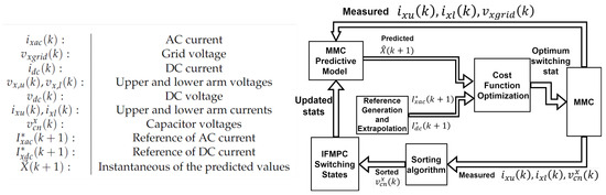
Figure 3.
Block diagram of the proposed FMPC.
Let us consider an example of an MMC featuring 10 SMs per arm, with a DC side voltage of 30,000 V. This implies that each SM ideally operates at 3000 V. Now, imagine a hypothetical scenario where, at a specific time, the anticipated number of upper and lower SMs to be inserted are two and eight, respectively. At this juncture, the capacitor voltages are depicted in Table 2 (these values have been recorded from simulation).
Table 2.
Capacitor voltages of the upper and lower arms.
The output voltage of this phase can be determined by applying the ideal capacitor voltage values, as described in Equation (8).
When utilising the actual capacitor voltages to compute the output voltage following the application of the sorting algorithm, the resulting expression is as follows:
The comparison of the above two results reveals a disparity between the predicted (ideal output voltage) and the actual voltage, amounting to 924.7 V (assuming the capacitor voltages remain constant during this brief interval). Consequently, this difference influences the adjustment of the output power.
In the proposed FMPC, actual capacitor voltages are employed to anticipate the switching states, aiming to select inserted SMs as closely aligned with the ideal values as possible. Utilising the same aforementioned example, to fulfill the output voltage requirement of 9000 V at this moment, the number of inserted SMs in the upper and lower arms will be adjusted. Specifically, there will be seven inserted SMs in the lower arm and one in the upper arm. Employing the same earlier equation, the outcome of the proposed FMPC will be:
Furthermore, the proposed approach allows for additional validation steps within the prediction stage to mitigate this shortfall in the output voltage. These supplementary steps involve replacing the initial bypassed SM with the final inserted SM for the same arm, followed by verification of whether the error persists. If so, the process continues by substituting the first two bypassed SMs with the last two inserted SMs and iterating this verification process, progressively increasing the number of SMs by one at each step, as depicted in Figure 4, until the desired value is attained. The exact number of these supplementary checks is not fixed and depends on the magnitude of errors encountered during normal predictions. However, these checks should not surpass a threshold that could impact the charging and discharging dynamics of the capacitors in each arm. These capacitors charge and discharge instantaneously based on the direction of the arm current. In this study, the maximum step value adopted was set at 30% of N to ensure that the capacitor voltages do not fluctuate by more than ±10% of their average voltage, .
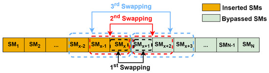
Figure 4.
Extra checking steps explanation for the inserted SMs per arm.
Continuing with the previous example, the extra checking steps will be:
As observed from the above results, the predicted voltage closely aligns with the ideal value. Despite the introduction of extra steps, which entail increased computational load, this assertion can be justified by three considerations. Firstly, as the number of SMs increases, voltage levels tend to converge, thus employing actual capacitor voltage values facilitates the identification of an optimal solution with greater precision and no extra validation steps. Moreover, the number of extra steps is relatively small, thus having minimal impact on the controller response time. Lastly, these extra steps can be computed for an individual control objective rather than all objectives included in the main cost function, thereby mitigating the computational burden.
The proposed FMPC incorporates the five aforementioned control objectives, utilising the discretisation models outlined in the preceding section to predict switching states. The flowchart outlining the proposed FMPC is depicted in Figure 5.
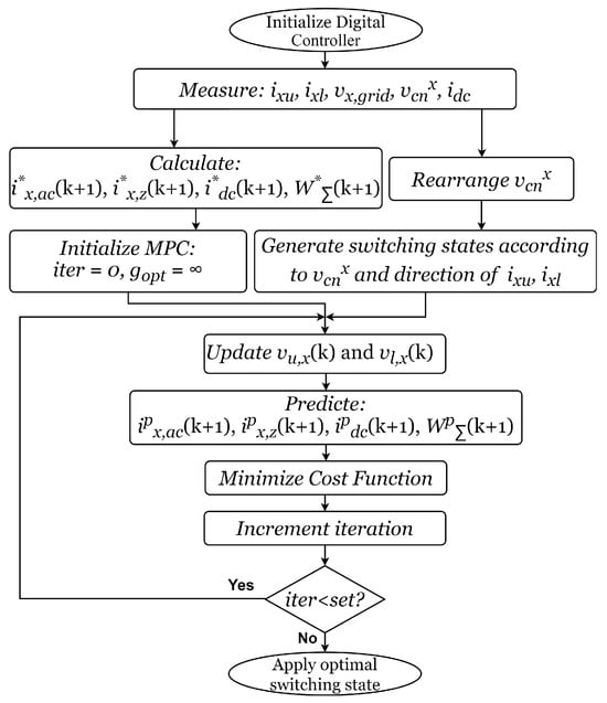
Figure 5.
Flowchart of the proposed FMPC.
The cost function in the proposed FMPC incorporates five control objectives, each assigned with three weighting factors denoted as , , and . In an MMC, the primary control objective is the AC current; thus, it holds the highest priority among other objectives, with its weighting factor fixed at 1 (). This paper suggests that the circulating current shares a similar priority with the DC current; hence, they are assigned identical weighting factors denoted as . Similarly, the arm and leg energies are deemed to have equal priority; thus, they receive the same weighting factor, denoted as . Determining the values of the weighting factors is crucial as it significantly influences the behaviour of the MPC. The following approach is adopted to calculate the weighting factors: Initially, the value of is varied from 0 to 1 using a lookup table while assuming = 0. The errors of both the DC and circulating currents corresponding to the variation in are recorded. Subsequently, the value of the second weighting factor, , is selected from the table based on the value that minimises the errors in both the DC and circulating currents. This process is then repeated for , and the errors of the energies are recorded. As a result, the cost function encompasses five control objectives with three priority weighting factors, as depicted in Equation (30).
5. HIL Setup
In this study, real-time hardware-in-the-loop (HIL) testing was conducted using both a PLEXIM RT Box 1 and RT Box 3 (Plexim GmbH, Zurich, Switzerland) to implement the MMC plant. Additionally, three LAUNCHXL-28379D Micro-controller units from Texas Instruments (TI) (Dallas, TX, USA) were utilised to control each phase of the MMC.
As is widely recognised, the MMC stands as one of the more intricate converter topologies, often incorporating numerous switching devices. Consequently, deploying it on an HIL platform can present challenges, necessitating implementation in multiple physical modes. In the context of the PLECS software (version 4.7.5), this entails multi-task implementation, where different segments of the model exchange information via voltage and current meters, as well as controlled voltage and current sources. The system is partitioned at a slowly varying state variable, such as the DC-Link. To validate the proposed FMPC, an MMC with four SMs per arm was employed. The measured signals obtained from the MMC are outlined in Table 3.
Table 3.
The measured signals from the MMC.
The RT Box 3 is the larger of the two, equipped with 32 analog output signals. Therefore, to accommodate all the analog signals in the MMC plant, both RT Box 1 and RT Box 3 need to be utilised. With three cores in the RT Box 3 and a single core in the RT Box 1, the MMC plant is divided into four tasks, allocated between these two RT Boxes, as illustrated in Figure 6.
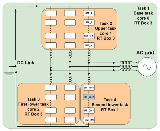
Figure 6.
Multitask distribution of MMC between RT Box 1 and RT Box 3.
In Figure 6, the green background denotes the base task, operating within Core 0 of RT Box 3. This task encompasses the AC grid, inductors, and resistances for each arm, as well as the inductance, resistance of the grid, and the DC bus source. The upper task covers all the SMs in the upper arms and is executed within Core 1 of RT Box 3. The first two lower arms are managed by Core 2 of RT Box 3, while RT Box 1 handles the final lower arm. Both RT Box 1 and RT Box 3 operate collectively as a single RT Box with four cores. The discretisation step size for both RT Box 1 and RT Box 3 is configured to 6 µs. Code Composer Studio (CCS) from TI was utilised for programming the MCUs. Figure 7 shows an overview of the HIL and control platforms employed for the MMC testing.
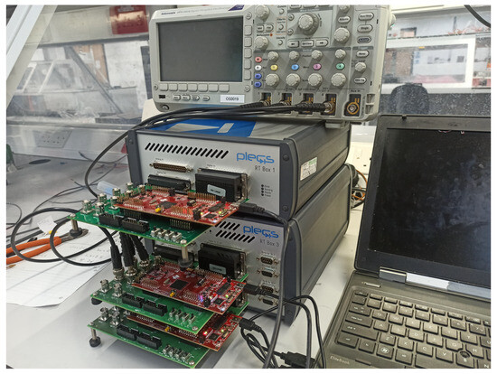
Figure 7.
RT Box 1 and RT Box 3 connection with three LAUNCHXL-F28379D.
6. Simulation Results
In the simulation section, an MMC with 10 SMs per arm was modelled. Table 4 presents a list of parameters utilised for the MMC in these evaluations. PLECS simulation software was employed to implement both the MMC and its control system. Three scenarios were taken into account to assess the proposed FMPC technique: steady-state response, dynamic response, and evaluation of its performance in the presence of 5th and 7th harmonic distortion in the AC grid.
Table 4.
Simulation parameters of MMC.
6.1. Steady-State Response
In the steady-state scenario, the primary focus lies on the main control objective, which is to track the reference current with optimal error tolerance, while ensuring that other control objectives are not compromised. The simulation results depicting the 3-phase output, upper arm, and lower arm current of phase A are presented in Figure 8. It is evident from the results that the MMC operating with the proposed FMPC exhibits stable steady-state behaviour, characterised by minimal harmonic content and high-quality output current.
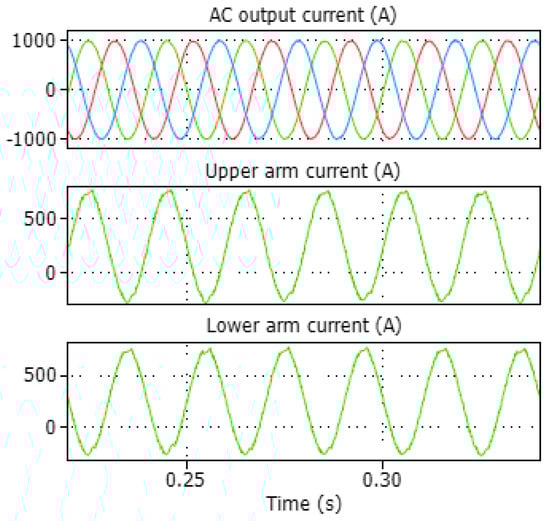
Figure 8.
3-phase output, upper arm, and lower arm currents of MMC with 10 SMs per arm.
Regarding the power quality analysis, Table 5 presents the total harmonic distortion (THD%) of both the AC and arm currents under steady-state conditions and with harmonic distortion in the AC grid. This facilitates the identification and evaluation of various power quality aspects of the system.
Table 5.
THD% with and without harmonics contents in AC side (simulation results).
In the spectrum analysis depicted in Figure 9, it is evident that the values of the low-order harmonics are relatively small, indicating minimal impact on the quality of the output current. Further reduction in harmonics can be achieved by reducing the sampling time.
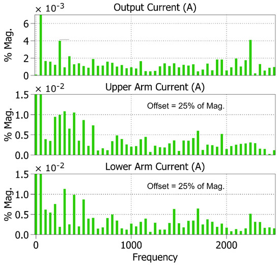
Figure 9.
Spectrum analysis of the 1-phase output current, upper and lower arms currents.
It is worth mentioning that the presence of the second harmonic component in the upper and lower arm currents (circulating current) does not affect the output current directly. The reason for that is the output current arises from the difference between these currents. However, the second circulating current contributes to an increase in the RMS value of the arm currents, leading to higher conduction and switching losses in the switching devices. Consequently, this can reduce the efficiency of the converter and the lifespan of the switching devices. To address this issue, the proposed FMPC eliminates the circulating current, as illustrated in Figure 10. This figure displays the waveforms of both the circulating current and the DC current during steady-state operation.
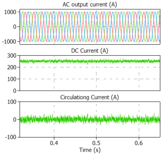
Figure 10.
3-phase output, DC, and circulating currents waveforms.
Another crucial aspect to consider is the equal distribution of energy storage among arms, which helps distribute stress evenly across the arms. Achieving this equilibrium involves the incorporation of the last two control objectives, namely, the leg’s energy and the arm’s energy, into the cost function (Equations (27) and (28)), along with utilisation of the sorting algorithm. A key indicator of energy balancing is the equalisation of capacitor voltages among arms, which can be observed through the fluctuation in capacitor voltages. Figure 11 depicts the capacitor voltages of phase A (upper and lower arms). The proposed method ensures that the capacitor voltages remain within an acceptable range, with fluctuations of less than ±10% of their average voltage, .
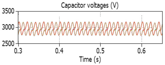
Figure 11.
Capacitor voltages fluctuations.
The proposed FMPC considerably reduced both the number of switching states and the computational burden.
6.2. Dynamic Response
The results obtained from the dynamic state assessment illustrate that the proposed FMPC demonstrates a rapid and accurate response in tracking the reference current without any overshoot, as shown in Figure 12. The step change of the output current from half value to the full load current occurs at t = 0.33 s. Additionally, the robustness of the proposed MPC is evident from Figure 13, where it exhibits a high response for the DC current and effectively suppresses the circulating current.
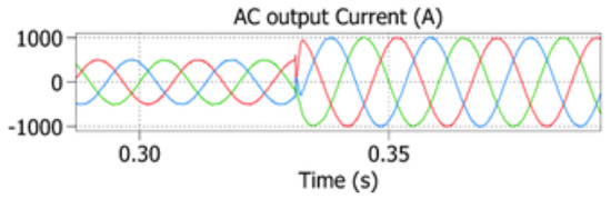
Figure 12.
Dynamic response of the 3-phase output current.
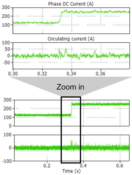
Figure 13.
Dynamic response of DC and circulating current.
As discussed in Section 4, the weighting factors play a pivotal role in shaping the behaviour of the control system, underscoring the importance of their selection. While the priority of the control objectives remains consistent during steady state, it is worth noting that during dynamic states, the prioritisation of control objectives may vary depending on the controller’s requirements. Fortunately, the proposed FMPC method exhibits a fast and smooth dynamic response, minimising the impact of such variation in the control objective priority.
6.3. Harmonic Content in AC Grid
The third scenario involves evaluating the control system’s performance under voltage disturbances introduced to the AC side, specifically the 5th and 7th order harmonics with a magnitude of 5% of the fundamental voltage. Figure 14 illustrates the grid voltage and output current. It is important to note that the results in Figure 14 assume that the output current is constrained to track a pure sinusoidal waveform and that, therefore, the harmonics appear as a disturbance to the control system. Overall, the proposed FMPC exhibits a fast response and satisfactory performance in managing all control objectives and disturbances. Moreover, the proposed method proves effective in reducing the THD% even when the harmonic content in the upper and lower arms is slightly increased, as indicated in Table 5.
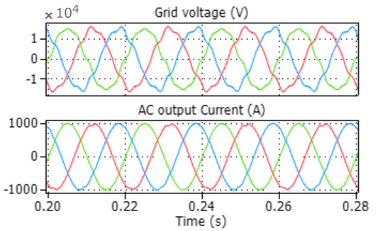
Figure 14.
Grid voltage and current during harmonics contents case.
Figure 15 shows the DC and circulating currents waveform when the 5th and 7th harmonics are injected in the AC grid.
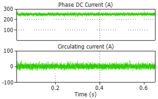
Figure 15.
DC and circulating currents when the 5th and 7th harmonics are injected in the AC grid.
7. HIL Results
To evaluate the performance of the proposed FMPC in a practical setting, real-time HIL testing was employed. The behaviour of the MMC with four SMs per arm was examined using the proposed FMPC. Table 6 enumerates the parameters utilised to implement the system. The same three scenarios mentioned previously were replicated to validate the robustness of the proposed MPC.
Table 6.
Real time HIL parameters of MMC.
7.1. Steady-State Performance
In contrast to simulation results, in the real-time HIL implementation, the control process must be completed within each sampling time interval, and the results applied in the next sample instance. In this way, the HIL behaviour closely resembles the demands of an experimental implementation, making delay time compensation crucial. To address this, a second-step prediction was implemented to compensate for the delay time in the control platform. Figure 16 displays the output voltage, while Figure 17 shows the output current. As depicted, the steady-state response closely resembles the simulation results with minor differences. The THD% values are listed in Table 7.
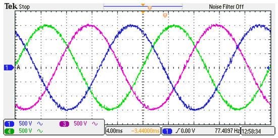
Figure 16.
3-phase output voltage of the MMC.
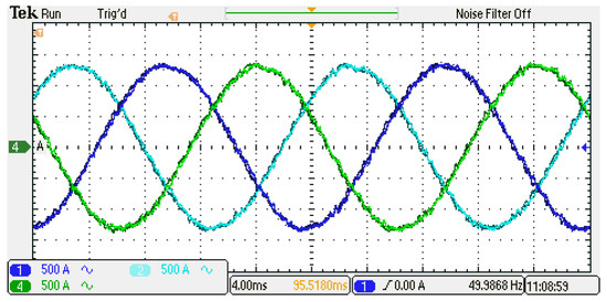
Figure 17.
3-phase output current.
Table 7.
THD% with and without harmonics contents in AC side (HIL results).
Figure 18 shows the DC and circulating currents; it is clearly seen that the low-order harmonic content is minimal and the high fluctuation comes from the switching of the MMC cells.
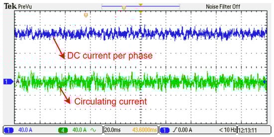
Figure 18.
DC and circulating currents per arm.
The fluctuations in capacitor voltages for phase A (upper and lower arm capacitors) are depicted in Figure 19. As is evident from the capacitor voltage figure, the fluctuations remain within the acceptable range of ±10% of the average voltage of the SMs.
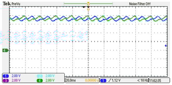
Figure 19.
Capacitor voltages of phase A.
The waveforms of the upper and lower arm currents are presented in Figure 20. The harmonic content within the currents falls within acceptable limits, as evidenced by Table 7.
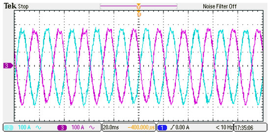
Figure 20.
Upper and lower arm currents.
In the HIL setup, general purpose input-output (GPIO) peripherals of the LAUNCHXL-F28379D controller were employed to trigger the switches of the MMC. This approach was adopted due to the absence of a PWM stage in the proposed MPC. The processing time for both the proposed FMPC and the sorting algorithm is 26.6 µs, as illustrated in Figure 21.
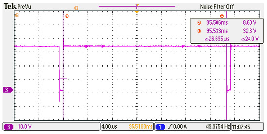
Figure 21.
Time of interrupt (computational time of FMPC).
It is important to note that the computational time varies based on several factors, such as the speed of the control platform, the number of SMs per arm, the script optimisation, etc. Therefore, the time mentioned above is not standard for an MMC with four SMs per arm; it is simply indicative of the time taken for the control interrupt period of the proposed MPC. Furthermore, in this study, the proposed MPC is not fully optimised, so shorter processing times could be achieved with additional optimisation steps. Nevertheless, the processing time sufficed for the application discussed in this paper, which primarily deals with low frequency.
7.2. Dynamic Response
To examine the dynamic performance of the proposed control algorithm, the amplitude of the output AC current was increased from 500 A to 1000 A. Figure 22 and Figure 23 depict the dynamic behaviour of the output current, DC current, and circulating current, respectively, using the proposed control algorithm. Both figures clearly illustrate that the MMC maintains stable operation and exhibits a fast response during the step change in AC current amplitude. The output AC current and DC current effectively track their respective references with a fast dynamic, as is evident in both figures. In Figure 23, the DC current steps from 125 A to 250 A in response to the change in AC current reference, ensuring that power balance is maintained between the DC and AC sides. The fluctuations in the SM capacitor voltages within the upper and lower arms remain stable and balanced, with variations kept within an acceptable range of under ±10% of their average value.
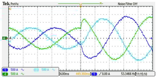
Figure 22.
Dynamic response of 3-phase output current.
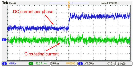
Figure 23.
Dynamic response of DC and circulating currents per arm.
7.3. Harmonics Content in the AC Grid
In this test, 5% of the 5th and 7th harmonics were added to the AC side grid voltage, as shown in Figure 24.
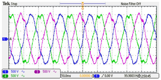
Figure 24.
Voltage grid when the 5% magnitude of the 5th and 7th harmonics are injected.
Figure 25 shows the HIL results of the AC current generated by the proposed FMPC algorithm when the AC grid voltage contains the aforementioned harmonics, aimed at assessing its robustness. As mentioned previously, the output current is tracking a pure fundamental frequency sinusoidal signal.
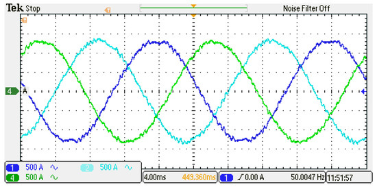
Figure 25.
Output current in case of harmonics contents.
Figure 25 demonstrates that the harmonics on the AC side have minimal impact on the algorithm. All the electrical parameters remain stable and show satisfactory steady-state performance.This is attributed to the model-based nature of MPC, where the grid voltage serves merely as a disturbance variable for the control algorithm, and its effects can be effectively mitigated with accurate measurement. Figure 26 illustrates that the MMC maintains stable operation even in the presence of grid harmonics. Both the DC and circulating currents exhibit fluctuations within an acceptable range.
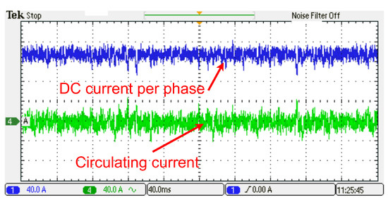
Figure 26.
DC and circulating current during harmonics contents.
It is worth mentioning that during the HIL implementation, the three MCUs operated autonomously, with a single MCU assigned to each phase. Despite the increase in both the upper and lower arm currents, the THD% of the output current remains within an acceptable range. Figure 27 depicts the upper and lower arm currents.
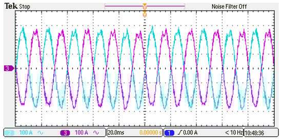
Figure 27.
Upper and lower arm current with harmonics included in the AC grid.
The harmonics on the AC side have an impact on the capacitor voltages, resulting in asymmetric voltage fluctuations around the average capacitor voltage, as observed by comparing Figure 17 and Figure 28. This phenomenon characterises the behaviour of storage devices in the presence of harmonics in the AC grid voltage. They attempt to compensate for the power inaccuracy, occasionally charging or discharging their voltage faster or slower than under normal operation. It is important to note that this behaviour has a diminished effect with an increase in the number of SMs per arm.
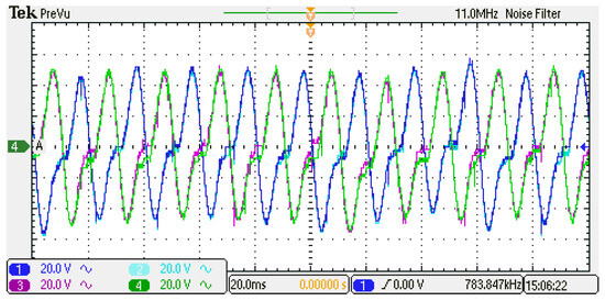
Figure 28.
Capacitor voltages.
8. Conclusions
This paper introduces a proposed folding MPC approach for MMCs, which reduces the number of switching states considered in the MPC algorithm to . The method integrates a sorting algorithm as a pre-processing stage, operating in parallel with the MPC stage without adding extra complexity to the control system, thus enabling more accurate predictions. Five control objectives are optimised through a unified cost function, including the AC current, DC current, circulating current, energy per arm, and leg energy.
The efficacy of the proposed folding MPC is verified through PLECS computer simulations and a real-time HIL implementation.
It is evident that the proposed FMPC technique for MMCs offers significant advantages in terms of both steady-state and dynamic performance, as well as robustness to harmonic distortions in the AC grid.
In the steady-state response analysis, the FMPC demonstrated exceptional capability in accurately tracking the reference current while minimising harmonic content and ensuring high-quality output current. Through simulation and HIL testing, it was observed that the FMPC effectively eliminates circulating currents, reduces THD%, and maintains balanced energy storage among the arms.
The dynamic response assessment further validated the effectiveness of the FMPC, showcasing rapid and precise tracking of the reference current without overshoot or instability. The controller exhibited robustness to changes in control objectives and maintained stable operation even during changes in load conditions.
Furthermore, the evaluation of harmonic content in the AC grid highlighted the FMPC’s ability to mitigate the effects of voltage disturbances introduced by harmonics. Both simulation and HIL results demonstrated the FMPC’s capability to maintain stable operation and satisfactory performance even under adverse grid conditions, such as the injection of 5th and 7th harmonic distortions.
Overall, the comprehensive analysis presented in this study underscores the effectiveness and versatility of the proposed FMPC technique for MMCs. Its ability to achieve optimal performance in various operating conditions, coupled with its computational efficiency and robustness, positions it as a promising solution for enhancing the performance and reliability of power electronic converters in modern power systems.
Author Contributions
Conceptualisation: H.K. initiated the research idea, while A.J.W., M.R. and P.Z. provided supervision and guidance throughout the conceptualisation process; methodology: H.K. developed the mathematical model, under the supervision of A.J.W., M.R. and P.Z. who contributed to the analysis; resources: the project was funded by A.J.W. and P.W.; writing—original draft preparation: H.K. drafted the initial version of the manuscript; writing—review and editing: A.J.W. and M.R. provided substantial editing and proofreading assistance; supervision: the project was supervised by A.J.W., M.R., P.Z. and P.W.; funding acquisition: funding for the project was acquired by A.J.W. and P.W. All authors have read and agreed to the published version of the manuscript.
Funding
This research received no external funding.
Data Availability Statement
The validation of the proposed idea in this study was conducted through simulation using PLECS software and real-time hardware-in-the-loop (HIL) implementation. However, no specific data were generated or used for analysis in this process. Therefore, the original contributions presented in the study are included in the article, further inquiries can be directed to Hussein or Alan at [hutakleef@gmail.com or alan.watson@nottingham.ac.uk].
Conflicts of Interest
The authors declare that they have no conflicts of interest.
Abbreviations
The following abbreviations are used in this manuscript:
| MPC | Model Predictive Control |
| MMC | Modular Multilevel Converter |
| FMPC | Folding Model Predictive Control |
| AC | Alternative Current |
| DC | Direct Current |
| HIL | Hardware-in-the-Loop |
| THD | Total Harmonics Distortion |
| SM(s) | Submodule(s) |
| HVDC | High-Voltage Direct Current |
| PWM | Pulse-Width Modulation |
| CCS-MPC | Continuous Control Set MPC |
| FCS-MPC | Finite Control Set MPC |
| PS-MPC | Sequential Phase-Shift Model Predictive Control |
| PS-PWM | Phase-Shift Pulse-Width Modulation |
| CMPCC | Compensatory Model Predictive Current Control |
| FFS-MPC | Fast Finite Level State MPC |
| MF-AC | Model-Free Adaptive Control |
| DD-PCC | Data-Driven-Based Predictive Current Control |
| FCS-MPC | Finite Control Set Model Predictive Control |
| CCS | Code Composer Studio |
| TI | Texas Instrument |
| MCU | Microcontroller |
References
- Poblete, P.; Neira, S.; Aguilera, R.P.; Pereda, J.; Pou, J. Sequential Phase-Shifted Model Predictive Control for Modular Multilevel Converters. IEEE Trans. Energy Convers. 2021, 36, 2691–2702. [Google Scholar] [CrossRef]
- Gong, Z.; Dai, P.; Yuan, X.; Wu, X.; Guo, G. Design and Experimental Evaluation of Fast Model Predictive Control for Modular Multilevel Converters. IEEE Trans. Ind. Electron. 2016, 63, 3845–3856. [Google Scholar] [CrossRef]
- Wang, Y.; Cong, W.; Li, M.; Li, N.; Cao, M.; Lei, W. Model predictive control of modular multilevel converter with reduced computational load. In Proceedings of the 2014 IEEE Applied Power Electronics Conference and Exposition—APEC 2014, Fort Worth, TX, USA, 16–20 March 2014; pp. 1776–1779. [Google Scholar] [CrossRef]
- Wang, J.; Tang, Y.; Lin, P.; Liu, X.; Pou, J. Deadbeat Predictive Current Control for Modular Multilevel Converters with Enhanced Steady-State Performance and Stability. IEEE Trans. Power Electron. 2020, 35, 6878–6894. [Google Scholar] [CrossRef]
- Dekka, A.; Wu, B.; Yaramasu, V.; Fuentes, R.L.; Zargari, N.R. Model Predictive Control of High-Power Modular Multilevel Converters—An Overview. IEEE J. Emerg. Sel. Top. Power Electron. 2019, 7, 168–183. [Google Scholar] [CrossRef]
- Böcker, J.; Freudenberg, B.; The, A.; Dieckerhoff, S. Experimental Comparison of Model Predictive Control and Cascaded Control of the Modular Multilevel Converter. IEEE Trans. Power Electron. 2015, 30, 422–430. [Google Scholar] [CrossRef]
- Nguyen, M.H.; Kwak, S. Simplified Indirect Model Predictive Control Method for a Modular Multilevel Converter. IEEE Access 2018, 6, 62405–62418. [Google Scholar] [CrossRef]
- Gutierrez, B.; Kwak, S.-S. Modular Multilevel Converters (MMCs) Controlled by Model Predictive Control with Reduced Calculation Burden. IEEE Trans. Power Electron. 2018, 33, 9176–9187. [Google Scholar] [CrossRef]
- Vatani, M.; Bahrani, B.; Saeedifard, M.; Hovd, M. Indirect Finite Control Set Model Predictive Control of Modular Multilevel Converters. IEEE Trans. Smart Grid 2015, 6, 1520–1529. [Google Scholar] [CrossRef]
- Wang, J.; Liu, X.; Xiao, Q.; Zhou, D.; Qiu, H.; Tang, Y. Modulated Model Predictive Control for Modular Multilevel Converters with Easy Implementation and Enhanced Steady-State Performance. IEEE Trans. Power Electron. 2020, 35, 9107–9118. [Google Scholar] [CrossRef]
- Zhang, F.; Li, W.; Joós, G. A Voltage-Level-Based Model Predictive Control of Modular Multilevel Converter. IEEE Trans. Ind. Electron. 2016, 63, 5301–5312. [Google Scholar] [CrossRef]
- Gong, Z.; Wu, X.; Dai, P.; Zhu, R. Modulated Model Predictive Control for MMC-Based Active Front-End Rectifiers Under Unbalanced Grid Conditions. IEEE Trans. Ind. Electron. 2019, 66, 2398–2409. [Google Scholar] [CrossRef]
- Zhou, D.; Yang, S.; Tang, Y. Model-Predictive Current Control of Modular Multilevel Converters with Phase-Shifted Pulsewidth Modulation. IEEE Trans. Ind. Electron. 2019, 66, 4368–4378. [Google Scholar] [CrossRef]
- Gao, X.; Pang, Y.; Xia, J.; Chai, N.; Tian, W.; Rodriguez, J.; Kennel, R. Modulated Model Predictive Control of Modular Multilevel Converters Operating in a Wide Frequency Range. IEEE Trans. Ind. Electron. 2023, 70, 4380–4391. [Google Scholar] [CrossRef]
- Wang, Z.; Yin, X.; Chen, Y. Model Predictive Arm Current Control for Modular Multilevel Converter. IEEE Access 2021, 9, 54700–54709. [Google Scholar] [CrossRef]
- Martin, S.P.; Li, H.; Anubi, O.M. Modulated MPC for Arm Inductor-Less MVDC MMC with Reduced Computational Burden. IEEE Trans. Energy Convers. 2021, 36, 1776–1786. [Google Scholar] [CrossRef]
- Martin, S.P.; Dong, X.; Li, H. Model Development and Predictive Control of a Low-Inertia DC Solid-State Transformer (SST). IEEE J. Emerg. Sel. Top. Power Electron. 2022, 10, 6482–6494. [Google Scholar] [CrossRef]
- Arias-Esquivel, Y.; Cárdenas, R.; Urrutia, M.; Diaz, M.; Tarisciotti, L.; Clare, J.C. Continuous Control Set Model Predictive Control of a Modular Multilevel Converter for Drive Applications. IEEE Trans. Ind. Electron. 2023, 70, 8723–8733. [Google Scholar] [CrossRef]
- Guo, P.; Xu, Q.; Yue, Y.; He, Z.; Xiao, M.; Ouyang, H.; Guerrero, J.M. Hybrid Model Predictive Control for Modified Modular Multilevel Switch-Mode Power Amplifier. IEEE Trans. Power Electron. 2021, 36, 5302–5322. [Google Scholar] [CrossRef]
- Yin, J.; Leon, J.I.; Perez, M.A.; Franquelo, L.G.; Marquez, A.; Vazquez, S. Model Predictive Control of Modular Multilevel Converters Using Quadratic Programming. IEEE Trans. Power Electron. 2021, 36, 7012–7025. [Google Scholar] [CrossRef]
- Chai, N.; Tian, W.; Gao, X.; Rodríguez, J.; Heldwein, M.L.; Kennel, R. Three-Phase Model-Based Predictive Control Methods with Reduced Calculation Burden for Modular Multilevel Converters. IEEE J. Emerg. Sel. Top. Power Electron. 2022, 10, 7037–7048. [Google Scholar] [CrossRef]
- Zhang, W.; Tan, G.; Zhang, X.; Wang, Q.; Zhang, J. Optimal Switching Sequence Model Predictive Control for Modular Multilevel Converter. IEEE Trans. Ind. Electron. 2023, 70, 5474–5483. [Google Scholar] [CrossRef]
- Liu, P.; Wang, Y.; Cong, W.; Lei, W. Grouping-sorting-optimized model predictive control for modular multilevel converter with reduced computational load. IEEE Trans. Power Electron. 2016, 31, 1896–1907. [Google Scholar] [CrossRef]
- Guo, P.; He, Z.; Yue, Y.; Xu, Q.; Huang, X.; Chen, Y.; Luo, A. A novel two-stage model predictive control for modular multilevel converter with reduced computation. IEEE Trans. Ind. Electron. 2019, 66, 2410–2422. [Google Scholar] [CrossRef]
- Ma, W.; Gong, D.; Guan, Z.; Li, W.; Meng, F.; Liu, X.; Wang, Y. Compensatory Model Predictive Current Control for Modular Multilevel Converter with Reduced Computational Complexity. IEEE Access 2022, 10, 106859–106872. [Google Scholar] [CrossRef]
- Liu, X.; Qiu, L.; Ma, J.; Fang, Y.; Wu, W.; Peng, Z.; Wang, D. A Fast Finite-Level-State Model Predictive Control Strategy for Sensorless Modular Multilevel Converter. IEEE J. Emerg. Sel. Top. Power Electron. 2021, 9, 3570–3581. [Google Scholar] [CrossRef]
- Wu, W.; Qiu, L.; Rodriguez, J.; Liu, X.; Ma, J.; Fang, Y. Data-Driven Finite Control-Set Model Predictive Control for Modular Multilevel Converter. IEEE J. Emerg. Sel. Top. Power Electron. 2023, 11, 523–531. [Google Scholar] [CrossRef]
- Liu, X.; Qiu, L.; Wu, W.; Ma, J.; Fang, Y.; Peng, Z.; Wang, D. Neural Predictor-Based Low Switching Frequency FCS-MPC for MMC with Online Weighting Factors Tuning. IEEE Trans. Power Electron. 2022, 37, 4065–4079. [Google Scholar] [CrossRef]
- Wang, S.; Dragicevic, T.; Gao, Y.; Teodorescu, R. Neural Network Based Model Predictive Controllers for Modular Multilevel Converters. IEEE Trans. Energy Convers. 2021, 36, 1562–1571. [Google Scholar] [CrossRef]
- Liu, X.; Qiu, L.; Wu, W.; Ma, J.; Fang, Y.; Peng, Z.; Wang, D. Event-Triggered Neural-Predictor-Based FCS-MPC for MMC. IEEE Trans. Ind. Electron. 2022, 69, 6433–6440. [Google Scholar] [CrossRef]
- Lesnicar, A.; Marquardt, R.; Lesnicar, A.; Marquardt, R. A New Modular Voltage Source Inverter Topology an Innovative Modular Multilevel Converter Topology Suitable for a Wide Power Range. 2003. Available online: https://www.researchgate.net/publication/205337714 (accessed on 5 April 2022).
- Imdadullah; Alamri, B.; Hossain, M.A.; Asghar, M.S.J. Electric Power Network Interconnection: A Review on Current Status, Future Prospects and Research Direction. Electronics 2021, 10, 2179. [Google Scholar] [CrossRef]
- HVDC Centre. HVDC Technology Capability (Version B). 2022. Available online: https://www.hvdccentre.com/wp-content/uploads/2022/04/SR-NET-HVDC-001-HVDC-Technology-Capability-vB.pdf (accessed on 5 May 2024).
- Siemens Energy Global GmbH & Co. KG. HVDC PLUS—The Decisive Step Ahead; References Erlangen, Germany. 2021. Available online: https://www.siemens-energy.com/global/en/home/products-services/product/hvdc-plus.html#Downloads-tab-3 (accessed on 5 March 2024).
- Pipelzadeh, Y.; Chaudhuri, B.; Green, T.; Wu, Y.; Pang, H.; Cao, J. Modelling and Dynamic Operation of the Zhoushan DC Grid: Worlds First Five-Terminal VSC-HVDC Project. In Proceedings of the International High Voltage Direct Current 2015 Conference, Seoul, Republic of Korea, 18–22 October 2015. [Google Scholar] [CrossRef]
- Rao, H. Architecture of Nan’ao multi-terminal VSC-HVDC system and its multi-functional control. CSEE J. Power Energy Syst. 2015, 1, 9–18. [Google Scholar] [CrossRef]
- Li, C.; Hu, X.; Guo, J.; Liang, J. The DC grid reliability and cost evaluation with Zhoushan five-terminal HVDC case study. In Proceedings of the 2015 50th International Universities Power Engineering Conference (UPEC), Stoke on Trent, UK, 1–4 September 2015; pp. 1–6. [Google Scholar] [CrossRef]
- National Research & Exploration Consortium. World’s First 5-Terminal VSC-HVDC Links. Available online: https://www.nrec.com/en/web/upload/2019/05/13/15577104617777z7mzh.pdf (accessed on 6 May 2024).
- Francos, P.L.; Verdugo, S.S.; Álvarez, H.F.; Guyomarch, S.; Loncle, J. INELFE—Europe’s first integrated onshore HVDC interconnection. In Proceedings of the 2012 IEEE Power and Energy Society General Meeting, San Diego, CA, USA, 22–26 July 2012; pp. 1–8. [Google Scholar] [CrossRef]
- Interconexion Electrica France España. Baixas—Santa Llogaia. INELFE. Available online: https://www.inelfe.eu/en/projects/baixas-santa-llogaia (accessed on 6 May 2024).
- Gu, X.; Liu, Y.; Xu, Y.; Yan, Y.; Cong, Y.; Xie, S.; Zhang, H. Development and qualification of the extruded cable system for Xiamen ±320 kV VSC-HVDC project. In Proceedings of the CIGRE, 08, Paris, France, 26–31 August 2018; pp. 1–10. [Google Scholar]
- Chandio, R.H.; Chachar, F.A.; Soomro, J.B.; Ansari, J.A.; Munir, H.M.; Zawbaa, H.M.; Kamel, S. Control and protection of MMC-based HVDC systems: A review. Energy Rep. 2023, 9, 1571–1588. [Google Scholar] [CrossRef]
- Tourgoutian, B.; Alefragkis, A. Design considerations for the COBRAcable HVDC interconnector. In Proceedings of the IET International Conference on Resilience of Transmission and Distribution Networks (RTDN 2017), Birmingham, UK, 26–28 September 2017; pp. 1–7. [Google Scholar] [CrossRef]
- Offshore Energy. Siemens Secures Order for COBRA HVDC Link. Available online: https://www.offshore-energy.biz/siemens-secures-order-for-cobra-hvdc-link/ (accessed on 6 May 2024).
- Ryndzionek, R.; Sienkiewicz, Ł. Evolution of the HVDC Link Connecting Offshore Wind Farms to Onshore Power Systems. Energies 2020, 13, 1914. [Google Scholar] [CrossRef]
- Planning and Implementation of an HVDC Link Embedded in a Low Fault Level AC System with High Penetration of Wind Generation. CIGRÈ Paris 2020. B4-16. Available online: https://api.semanticscholar.org/CorpusID:232374759 (accessed on 6 May 2024).
- Sennewald, T.; Linke, F.; Sass, F.; Westermann, D. Curative Actions by embedded bipolar HVDC-interconnections. In Proceedings of the International ETG-Congress 2019, ETG Symposium, Esslingen, Germany, 8–9 May 2019; pp. 1–6. [Google Scholar]
- NS Energy Business. Zhangbei VSC-HVDC Power Transmission Project. Available online: https://www.nsenergybusiness.com/projects/zhangbei-vsc-hvdc-power-transmission-project/# (accessed on 6 May 2024).
- Zhang, Y.; Wang, S.; Liu, T.; Zhang, S.; Lu, Q. A traveling wave-based protection scheme for the bipolar voltage source converter based high voltage direct current (VSC-HVDC) transmission lines in renewable energy integration. Energy 2021, 216, 119312. [Google Scholar] [CrossRef]
- NS Energy Business. North Sea Link Interconnector Project. Available online: https://www.nsenergybusiness.com/projects/north-sea-link-interconnector-project/# (accessed on 6 May 2024).
- Saeedifard, M.; Iravani, R. Dynamic performance of a modular multilevel back-to-back HVDC system. IEEE Trans. Power Deliv. 2010, 25, 2903–2912. [Google Scholar] [CrossRef]
- Isik, S.; Alharbi, M.; Bhattacharya, S. An Optimized Circulating Current Control Method Based on PR and PI Controller for MMC Applications. IEEE Trans. Ind. Appl. 2021, 57, 5074–5085. [Google Scholar] [CrossRef]
- Yaramasu, V.; Wu, B. Mapping of Continuous-Time Models. In Model Predictive Control of Wind Energy Conversion Systems; IEEE: Piscataway, NJ, USA, 2017; pp. 207–234. [Google Scholar] [CrossRef]
- Kadhum, H.T.; Alan, W.; Marco, R.; Pericle, Z.; Patrick, W. Model predictive control with reduced computational burden of modular multilevel converter. In Proceedings of the IET Conference Proceedings, Institution of Engineering and Technology, Brussels, Belgium, 23–24 October 2023; pp. 357–364. [Google Scholar] [CrossRef]
Disclaimer/Publisher’s Note: The statements, opinions and data contained in all publications are solely those of the individual author(s) and contributor(s) and not of MDPI and/or the editor(s). MDPI and/or the editor(s) disclaim responsibility for any injury to people or property resulting from any ideas, methods, instructions or products referred to in the content. |
© 2024 by the authors. Licensee MDPI, Basel, Switzerland. This article is an open access article distributed under the terms and conditions of the Creative Commons Attribution (CC BY) license (https://creativecommons.org/licenses/by/4.0/).