Enhancing Heat Transfer in Mini-Scale Liquid-Cooled Heat Sinks by Flow Oscillation—A Numerical Analysis

Abstract

Oscillatory baffled flows (OBFs) provide a combined active and passive means of achieving convective heat transfer enhancement, and previous studies at large scale have demonstrated the heat transfer benefits of OBFs. To date, however, this technology has not been scaled down for the purpose of heat sink performance enhancement. Presented in this study is a numerical investigation of a single baffled channel with a hydraulic diameter of 2.8 mm, containing gate baffles, with a 50% open area, which are spaced 7.5 mm apart. Three net-flow rates were investigated while varying the oscillation conditions by varying the oscillation amplitude (3 mm to 7 mm) and by varying the oscillation frequency (0 to 8 Hz). Increasing the oscillation intensity had a greater impact on the Nusselt number compared to simply increasing the net-flow rate, with Nu enhancements of up to 330% observed when imposing oscillatory flow on a purely steady flow. Ideal operating conditions were identified by grouping the data by velocity ratio ($\mathsf{\Psi }$) and graphing the theoretical pumping power against the thermal resistance of the channel. The highest Nu enhancement of 330% was achieved for a net-flow Reynolds number (${Re}_n$) of 165, oscillatory amplitude of 5 mm and a frequency of 8 Hz. Ideal operating conditions can be predicted by selecting conditions with $\mathsf{\Psi }$ > 1. A flow with a ${Re}_n$ of 46, $\mathsf{\Psi }$ of 7 and Nu = 12 required the same pumping power as a flow with a ${Re}_n$ of 165, $\mathsf{\Psi }$ of 0.65 and Nu = 6.

1. Introduction

With AI technology becoming ever more integrated into 21st century lives, the computational power of personal electronic devices and data centres are increasing year on year. Maintaining the compact size of integrated circuit boards (ICBs) while optimising performance results in increased chip densities with larger heat fluxes. It has previously been observed that an increase in 10 °C operation temperature can lead to a reduction in lifespan by 50% [1], but the directory is accelerating towards miniaturisation. In 2006, it was predicted that by the year 2020, microchips would reach a transistor density of 100 million transistors per mm², which has been updated to, by the year 2047 we will start to see microchips with 100 billion transistors per mm² appearing on the market [2]. This continual development necessitates the co-development of a new generation of high flux, cooling technologies.

Research in this area has been broad, with mooted solutions including mini-channel and microchannel heat sinks, some using single phase flow (usually liquids) and others utilising flow boiling. It is broadly accepted that it will be difficult to find a general, one-size-fits-all solution to this issue and that a range of different technological solutions will be required depending on situational requirements.

Previously, mini-channel development has focussed on modifying the geometry of the flow path, either via further miniaturisation to the micro-scale [3] or via the addition of features to promote flow disturbance and/or to increase surface area. Marzougui et al. (2016) investigated replacing parallel, straight channels with a single serpentine channel with a common hydraulic diameter, while further investigating the reduction in the hydraulic diameter of the serpentine channel design. The serpentine channel with a hydraulic diameter of 3 mm showed a four-fold increase in the heat transfer coefficient compared to the parallel channels. When reducing the hydraulic diameter of the channels from 3 mm to 2 mm, there was a less pronounced enhancement in the heat transfer coefficient [4]. The enhancement caused by the replacement of the parallel channels with the serpentine channels could be attributed to poor flow distribution between the parallel channels. To mitigate the effects of poor flow distribution, there is a large body of research investigating the inlet features that distribute the flow more uniformly between the channels [5,6,7,8].

The designs of parallel channels have also been investigated with the addition of dimples on the channel base to initiate swirling flows [9]. Straight parallel channels have also been replaced with a bank of sinusoidal wavy channels that lead to a doubling of the heat transfer coefficient compared to straight, parallel channels [10]. Less impactful designs have been compared where the maximum enhancement was 12.5% in the heat transfer coefficient where a parallel, zig-zag channel design was compared to equivalent straight parallel channels [11]. Parallel, zig-zag channels have been shown to be advantageous to designs that use pin fins as flow disrupters, showing both a 55% performance enhancement in the heat transfer coefficient compared to the pin fin design, along with a slight improvement in the pressure drop [12].

Various studies have also investigated the enhancement of the heat transfer properties of the working fluid. Both evaporative systems and liquid-forced convection have been widely investigated, with an overlap in performance for these two methods [13]. An enhancement method of interest is the utilisation of nanofluids, which are fluids that contain particles of less than 100 nm in diameter [14]. Nada et al. (2022) compared water to aluminium oxide nanofluid and concluded that the nanofluid containing Al₂O₃ flowing through a serpentine channel showed a 20% improvement in the heat transfer coefficient over pure water coolant [15]. However, Alkasmoul et al. (2018) [16] investigated water-based nanofluids containing Al₂O₃, TiO₂ and CuO and concluded that the addition of the nanoparticles has a detrimental effect on the heat transfer performance of the heat transfer systems when compared to water. This is due to the increase in the kinematic viscosity of the fluid via the addition of the nanoparticles; thus, for an equivalent Reynolds number to pure liquid-water flows, a higher flow velocity of the nanofluids is required. This increases both the required pump duty and the pressure drop of the system, leading the authors to conclude that the addition of nanoparticles to water-cooled systems is not beneficial for heat transfer performance [16].

As an alternative to a bank of parallel channels where there are issues achieving effective flow distribution between the channels, Al-Neama et al. (2018) investigated a single serpentine channel with water as the working fluid. The lowest thermal resistance that they reported was 2.3 × 10⁻¹ K·W⁻¹, at a ${Re}_n$ of 4500, which had the drawback of returning the highest pressure drop of 40 kPa [17]. A previous study also by Al-Neama et al. investigated similar serpentine channels where the walls of the channel were replaced with chevrons. This resulted in an approximately 10% increase in Nu for the chevron-serpentine channel, compared to the closed serpentine channel, while also reducing the pressure drop by around a third [18].

So far, the methods for optimising liquid-cooling described all utilised a steady-flow, with no study observed that investigated the employment of Oscillatory Baffled Flows (OBFs) for the purpose of heat sink optimisation. OBFs combine the flow disturbance caused by the presence of flow disrupters, with the superimposition of oscillatory flow onto the net fluid flow. OBFs have been demonstrated to enhance heat transfer at larger scales with an early demonstration of the heat transfer performance of OBFs being reported by Mackley et al. (1995) where they showed that oscillatory flow through a baffled pipe increases the Nu by ten-fold compared to a steady flow through a smooth pipe with a diameter of 12 mm [19]. This enhancement is significantly larger than those observed using passive enhancement methods alone. This work was expanded upon by Ahmed et al. (2018), which also showed a ten-fold enhancement in the heat transfer coefficient within an oscillatory baffled reactor when central baffles were used as the flow disruptors, compared to a steady flow [20]. OBF reactors and heat exchangers enhance fluid mixing by decoupling the fluid mixing effects from the net-flow velocity, thus allowing for plug flow at low net-flow Reynold’s numbers, which are usually associated with laminar flow (${Re}_n$< 2300) [19,20,21,22,23,24]. This facilitates turbulent-like transport characteristics at flow rates which would be considered laminar under steady flow conditions [19,20,21,22,23,24,25,26]. In addition to the positive effect that OBFs have on heat transfer at the larger scale, OBFs have also been observed to show energy recovery on the downstroke of the oscillations at low oscillation frequencies [19], minimising the additional pumping requirement.

To the best of the authors’ knowledge, OBFs have not yet been considered for heat transfer enhancements in heat sinks. If the enhancement effects observed at larger scales are also observable at these smaller scales, then these designs have the potential to be a step change in heat sink design. However, the design of such heat sink channels are not directly comparable to the larger scale systems previously characterized, with the larger scale systems being tubular in design and the heat sinks having a rectangular cross-section [27,28].

This paper presents a feasibility study of this technology, where a single baffled channel was investigated numerically and key performance indicators such as pressure drop, thermal resistance and heat transfer coefficient reported. The channel had a hydraulic diameter (D_h) of 2.86 mm, with simple “gate baffles” providing flow disturbance. This is a first-pass investigation intended to ascertain whether OBFs at this scale retain the enhancement advantage when mixing effects may have less of an impact on heat transfer.

2. Methodology

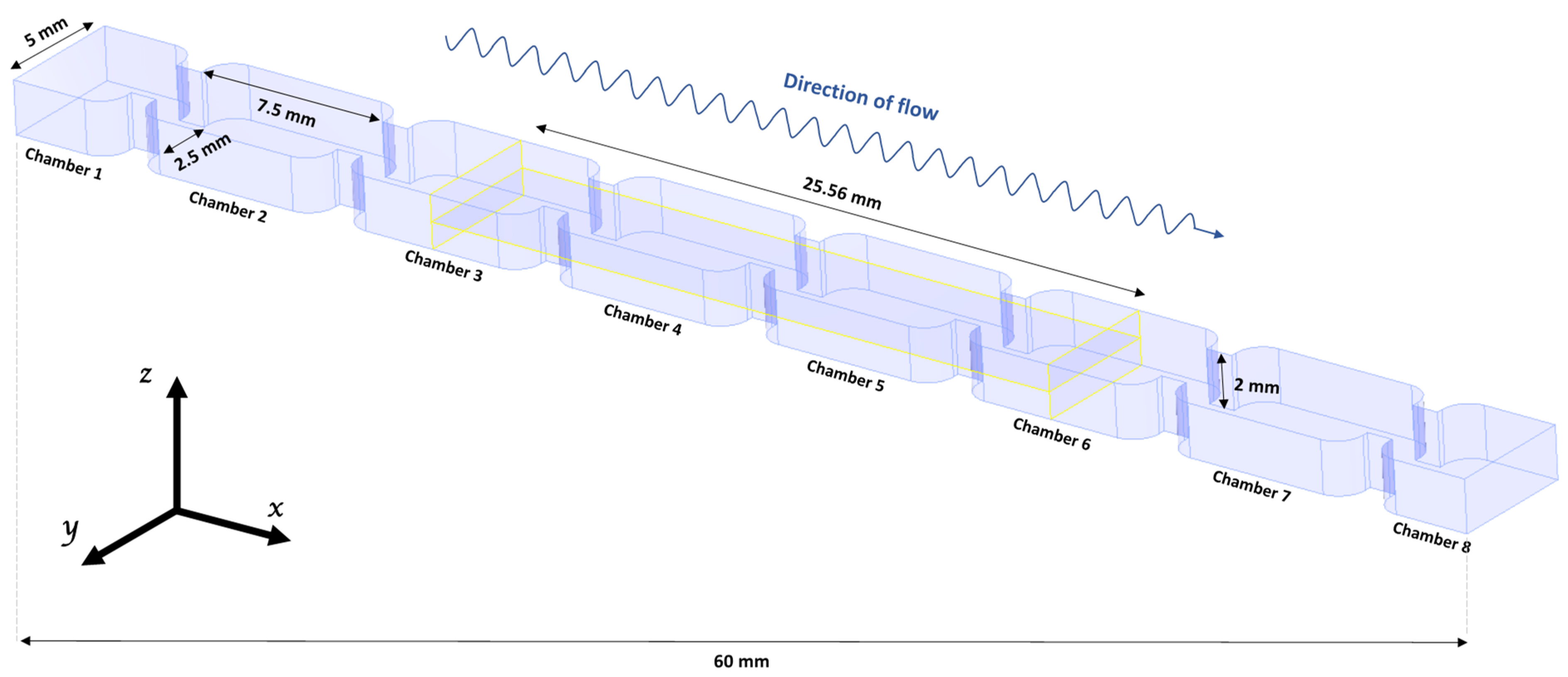
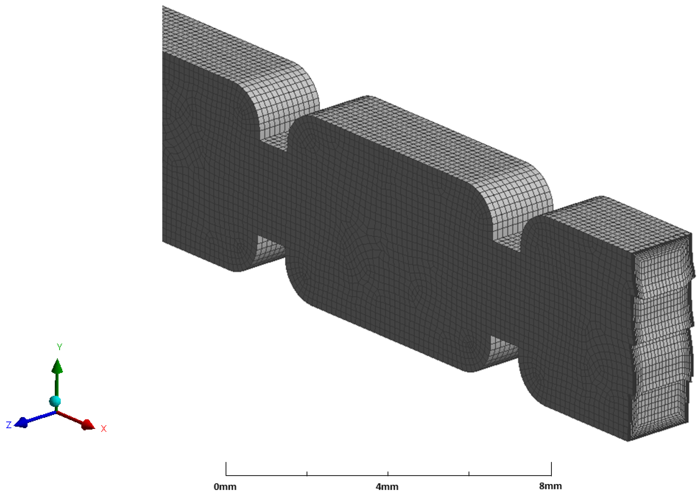
2.1. Geometry, Mesh and Model

The Computational Fluid Dynamics (CFD) software Ansys FLUENT (2022) was used for the analysis. CFD involves solving the Navier-Stokes equations, expressed in vector form by Equation (1) (Versteeg & Malalasekera, 2007, p. 23 [29]).

$$\rho \frac{\partial \stackrel{⃑}{U}}{\partial t}+\stackrel{⃑}{U}·\nabla \stackrel{⃑}{U}-{\mu \nabla }^2\stackrel{⃑}{U}=-\nabla p$$

(1)

where $\stackrel{⃑}{U}$ is the three-dimensional velocity field, $p$ (Pa) is the pressure and $\mu$ is the dynamic viscosity (Pa·s). Equation (1) represents three equations, with four unknowns, $u$ (velocity in the x-direction, m·s⁻¹), $v$ (velocity in the y-direction, m·s⁻¹), $w$ (velocity in the z-direction, m·s⁻¹) and $\rho$ (fluid density (kgm⁻³)). The Navier-Stokes equation can be directly solved for the velocity fields, but for $p$ Equation (1) it requires an iterative process using the continuity equation (Equation (2)) as a check (Versteeg & Malalasekera, 2007, p. 11 [29]).

$$\nabla ·\stackrel{⃑}{U}=0$$

(2)

Once Equation (2) is satisfied to a pre-set tolerance, then the result is said to have converged.

As the current study is also investigating heat transfer, a fifth unknown of temperature, $T$, must also be calculated using the energy equation as shown in Equation (3) (Versteeg & Malalasekera, 2007, p. 20 [29]).

$$\frac{\partial \left(\rho c_{p}T\right)}{\partial t}+\nabla ·\left(\rho \stackrel{⃑}{U}{c}_{p}T\right)=\nabla ·\left(\kappa \nabla T\right)+S_e$$

(3)

This is the internal energy form of the energy equation, which FLUENT utilises when using a pressure-based solver. The term $S_e$ is known as the source term and is governed by the wall temperature and inlet temperature in the current study.

The CFD solver selected for this investigation was the laminar Ansys FLUENT 2022, using the finite volume discretisation scheme and the SIMPLEC scheme with a skewness correction factor of 1. The least squares cell-based gradient function was used, with the PRESTO! scheme for pressure calculation. The second-order upwind discretisation for the momentum and energy calculations and the second-order implicit transient formulation was utilised for the transient energy and velocity terms. These settings were selected on consultation of previous modelling heat transfer systems using oscillating or pulsatile flows [17,27]. This methodology follows that of Solano et al. (2012) [28] and McDonough et al. (2019) [30] who investigated oscillatory baffled flows at a mesoscale using CFD, validated using PIV. Here, the authors used the laminar viscous model as with these discretisation schemes and a fine enough grid; the laminar solver can produce a solution akin to a Direct Numerical Simulation (DNS) [30,31].

The model of the heat sink channel is shown in Figure 1. In lieu of tube inserts that commonly provide flow disturbance in larger scale OBFs, “gate baffles” are included as features of the channel walls. The dimensions of the model were constrained by what could be readily manufactured using traditional, relatively low-spec CNC milling techniques. The channel has a maximum width of 5 mm and a minimum width (in the “gate”) of 2.5 mm. The channel depth was 2 mm, and the radius of the corners of the baffles were 1 mm. The spacing between the gate baffles is 1.5×, the maximum channel width. The total length of the channel was 60 mm. This was divided into eight chambers by baffles with a thickness of 1 mm and with a cross-sectional opening fraction of the channel of 0.60.

The geometry as shown in Figure 1 is compartmentalised into chambers by the baffles, with two truncated chambers on either end of the channel. To extract the temperature data from the CFD simulation, two planes were inserted in the geometry perpendicular to the direction of the net flow. These were situated in the centres of chamber 3 and chamber 6 to avoid the influences of the inlet and outlet boundary conditions. A study of velocity vectors confirmed that the flow was quasi-developed by chamber 3. Here, key data were extracted, including velocity vectors, temperature and pressure. A third plane was inserted into the centre of the channel at a depth of 1 mm in the z-direction, ranging from the centre of the third chamber to the centre of the sixth chamber. This enabled the flow patterns at the centre of the flow field to be analysed. The channel geometry, along with the location of the described calculation planes, are displayed in Figure 1.

The geometry was created using Design Modeller and meshed using the inbuilt, automatic Ansys meshing tool. The multizone setting was used which produced a structured, hexahedral mesh. A grid independence study determined that the average face size should be 0.18 mm, producing a very fine mesh containing 405,856 nodes and 390,272 cells. This mesh is displayed in Figure 2.

The mesh displayed in Figure 2 was selected by performing a grid independence study. Five cell sizes were tested to find the maximum cell size where the pressure drop and Nusselt number of the channel were independent from further reductions in cell size. The cell sizes chosen were 0.15 mm, 0.18 mm, 0.28 mm, 0.3 mm and 0.75 mm. Results of this analysis are discussed in Section 3.1.

Table 1. Boundary conditions used for the grid independence study.

Inlet Fluid Temperature (°C)	5
Wall Temperature (°C)	60
Initial System Temperature (°C)	5
Working Fluid	Water

shows the boundary conditions applied in the grid independence study and all subsequent simulations.

For the grid independence study, the oscillation frequency was selected as 46.5 Hz, with an oscillation amplitude of 3 mm. This frequency was the highest used in test simulations. The net-flow Reynolds number was 233, which corresponded to 82 mm·s⁻¹, which represents the maximum net-flow and oscillatory conditions combination.

To model the flow oscillation, an unsteady velocity profile was modelled using an expression for an oscillatory velocity as shown in Equation (4).

$$u\left(t\right)=u_n+2\pi f{x}_o\sin \left(2\pi ft\right)$$

(4)

This profile is the sum of a net-flow, steady component and an oscillating component, where $u_n$ is the superficial net-flow velocity defined by the net volumetric flow divided by the open cross-sectional area of the channel, (m·s⁻¹), $f$ is the frequency in Hz, $x_o$ is the centre-to-peak oscillation amplitude (mm) and $t$ is time (s). $u\left(t\right)$ is the velocity at time $t$ (m·s⁻¹). It should be noted that the time-averaged velocity (and therefore flowrate) is always positive to facilitate continuous heat removal (see example plots of velocity vs. time in Figure 3).

A timestep of 0.001 s was used for all simulations, which ensured that the Courant number was less than 1 for all simulations. The simulation time was 5 s, with quasi-steady state achieved within the first two seconds. Data were collected between the 3rd and 4th second of the simulation time.

The channel walls were defined with no-slip boundary conditions, and a constant wall temperature of 60 °C was set, as the electronic failure rate is compared to the failure rate of electronics at 75 °C [32], so it was decided to simulate the system below this value. The system had a zero-pressure outlet, and the outlet temperature was defined via a function to equal the temperature calculated in the final layer of the mesh. Finally, physical properties such as thermal conductivity, density and viscosity are all assumed constant and set by the Ansys^® Fluent software.

Equations (5)–(7) describe the dimensionless groups that are commonly used to describe oscillatory flow [30,33]. Equation (5) is the net-flow Reynolds number which uses the superficial net-flow velocity of the flow as the velocity term ($u_n$). This term gives an indication of whether the net-flow velocity of the flow is sufficient to induce turbulence. Equation (6) is the oscillatory-flow Reynolds number, where the velocity term is replaced with the maximum forward velocity of the oscillation cycle ($2\pi f{x}_o$). Equation (7) is the velocity ratio, which is the ratio of the maximum forward-stroke oscillatory velocity to the net-flow velocity. This determines whether the flow is net-flow dominant or oscillatory-flow dominant. At a velocity ratio of 0, only net-flow conditions exist, and a velocity ratio of 1 returns a purely pulsatile flow where the flow direction is constantly positive in the flow direction, with the minimum velocity dropping to 0 m·s⁻¹. When the velocity ratio increases beyond 1, the oscillatory component induces flow reversal on the oscillation downstroke. This effect is demonstrated in Figure 3. Equation (8) is the total Reynolds number, where the velocity term is the summation of the superficial net-flow velocity and the maximum forward velocity of the oscillation cycle.

$${Re}_n=\frac{\rho u_n{D}_h}{\mu }$$

(5)

$${Re}_o=\frac{2\pi f{x}_o\rho D_h}{\mu }$$

(6)

$$\mathsf{\Psi }=\frac{{Re}_o}{{Re}_n}$$

(7)

$${Re}_T=\left(u_n+2\pi f{x}_o\right)·\frac{\rho D_h}{\mu }$$

(8)

Equations (5)–(7) are the three dimensionless groups that are commonly used to describe the hydrodynamics of oscillatory flow through a baffled channel. $D_h$ is the hydraulic diameter of the channels (m), $\mu$ is the fluid viscosity (Pa·s), $x_o$ is the oscillation amplitude (m) and $f$ is the oscillation frequency (Hz).

Three net-flow Reynolds (${Re}_n$) numbers of 46, 165 and 233, which corresponded to a velocity of 16 mm·s⁻¹, 57 mm·s⁻¹ and 82 mm·s⁻¹, were investigated. The corresponding mass flowrates were 0.15 g·s⁻¹, 0.57 g·s⁻¹ and 0.82 g·s⁻¹, respectively. Three oscillation amplitudes of 3 mm, 5 mm and 7 mm and a frequency range of 0–8 Hz were investigated for each ${Re}_n$. Further simulations were necessary using a higher frequency range to investigate the plateau in Nu at higher $\mathsf{\Psi }$ for ${Re}_n$ of 165 and 233. This required a $\mathsf{\Psi }$ range of 0 to 10, requiring frequencies up to 46 Hz. The initial parameter space ($x_o$ 3–7 mm, $f$ 0–8 Hz) was based on what is theoretically achievable using commercially available syringe pumps that have been utilised previously in oscillatory flow reactor studies [25,33], with higher frequencies only included in some of the models for completion of the analysis.

2.2. Data Analysis

The temperature data were collected and then exported from the planes in chamber 3 and chamber 6 and taken as the inlet temperature ($T_i$) and outlet temperature ($T_o$), respectively. The time-averaged film heat transfer coefficient ($\overline{h}$) was calculated using Equation (9).

$$\overline{h}=\frac{c_p\dot{m}\mathsf{\Delta }T}{A{\mathsf{\Delta }T}_{Av}}$$

(9)

where

$$\mathsf{\Delta }T=T_o-T_i$$

(10)

and

$${\mathsf{\Delta }T}_{Av}=T_{wall}-\frac{T_i+T_o}{2}$$

(11)

The convective thermal resistance, $R$, is found using Equation (12).

$$R=\frac{1}{\overline{h}A}$$

(12)

$c_p$ is the heat capacity of water (4182 J·kg⁻¹·K⁻¹), and $\dot{m}$ is the mass flowrate of the water which was calculated from $u_n$ and $A$ is the inner surface area of the channel walls between the two central planes situated in chamber 3 and chamber 6 (Figure 1, 357.1 × 10⁻⁶ m², obtained from Design Modeller). The time-averaged Nusselt number was then calculated using Equation (13).

$$\overline{Nu}=\frac{\overline{h}{D}_h}{\kappa }$$

(13)

$\kappa$ is the thermal conductivity of water (0.6 W·m⁻¹·K⁻¹). The time-averaged Nusselt number is used as it gives a measure of the overall cooling performance of the channel. This averaged value can be readily compared to the heat transfer performance of steady flow conditions, allowing for a ‘pseudo-steady state’ comparison of the channels as the Nu will vary over an oscillation cycle. This variation has previously been determined to not lead to significant, observable effects [28].

The pressure drop across the flow area was calculated by subtracting the area average for the pressure recorded in the central plane of chamber 3 ($P_i$) from area average for the pressure recorded at the central plane in chamber 6 ($P_o$).

For steady flow, the pumping power can be calculated by multiplying the pressure drop by the volumetric flowrate (Equation (14)):

$$P_p=\mathsf{\Delta }P\times Q$$

(14)

where $\mathsf{\Delta }P$ is the pressure drop across the flow path (Pa) and Q is the volumetric flowrate (m³·s⁻¹).

For oscillatory flows, the power density, ${\epsilon }_v$, was calculated using Equation (15) as originally described by Mackley et al. [19]. The pumping power, $P_p$, is then calculated by multiplying the ${\epsilon }_v$ by the volume of the test section, according to Equation (16).

$${\epsilon }_v=\frac{u_n{\mathsf{\Delta }P}_n}{\left(V/A\right)}+\frac{\omega x_o{\mathsf{\Delta }P}_o\cos \left(\delta \right)}{2\left(V/A\right)}$$

(15)

$$P_p={\epsilon }_{v}V$$

(16)

${\mathsf{\Delta }P}_n$ is the net pressure drop, ${\mathsf{\Delta }P}_o$ is the maximum centre-to-peak pressure drop fluctuation, $\omega$ is the oscillation angular frequency (rad·s⁻¹), $\delta$ is the phase shift between the pressure signal and the velocity signal, calculated by following the procedure as described in [19,27], and $V$ is the volume (m³) of the channel between the planes present in chamber 3 and chamber 6 (Figure 1).

For flow visualisation, 2D velocity vectors are extracted from FLUENT from the central plane straddling the centre of the channel between chambers 3 and 6 (Figure 1). The velocity magnitudes of these 2D velocity vectors were calculated using Equation (17) and used for flow visualisation by creating velocity contour plots.

$$\left|\underset{\_}{{\mathit{U}}_{x,y}}\right|=\sqrt{{U_x}^2+{U_y}^2}$$

(17)

3. Results and Discussion

3.1. Grid Independence Study

To determine whether the mesh density (Figure 2) has a negligible impact on the simulation, a grid independence study was undertaken to find the minimum grid density that could produce a consistent solution for Nu and pressure drop. A total of 5 meshes were considered, with details presented in

Table 2. Details of the grid tested for independence studies.

Mesh Number	Inflation Layers	Element Size (mm)	Channel Volume (mm3)	Number of Elements	Elements per mm3
1	0	0.28	552.28	30,056	54.42
2	5	0.75	552.28	43,068	77.98
3	10	0.3	552.28	128,362	232.42
4	10	0.18	552.28	389,504	705.27
5	10	0.15	552.28	570,812	1033.56

. The results of this analysis are displayed in Figure 4.

Figure 4B shows that the pressure drop calculation stabilises after mesh number 4. The effect of the mesh is less impactful on the Nusselt number calculation (Figure 4A), as mesh independence appears to have been achieved after mesh number 2.

On analysis of Figure 4, mesh 4 was deemed to be independent of the simulation results. The relative difference between mesh number 4 and mesh number 5 was 2.85% for Nu and 0.68% for pressure drop. The calculations for all future simulations were solved in parallel using between three and five real cores and one GPU, with mesh 4. Each calculation took between 14 and 22 h to complete.

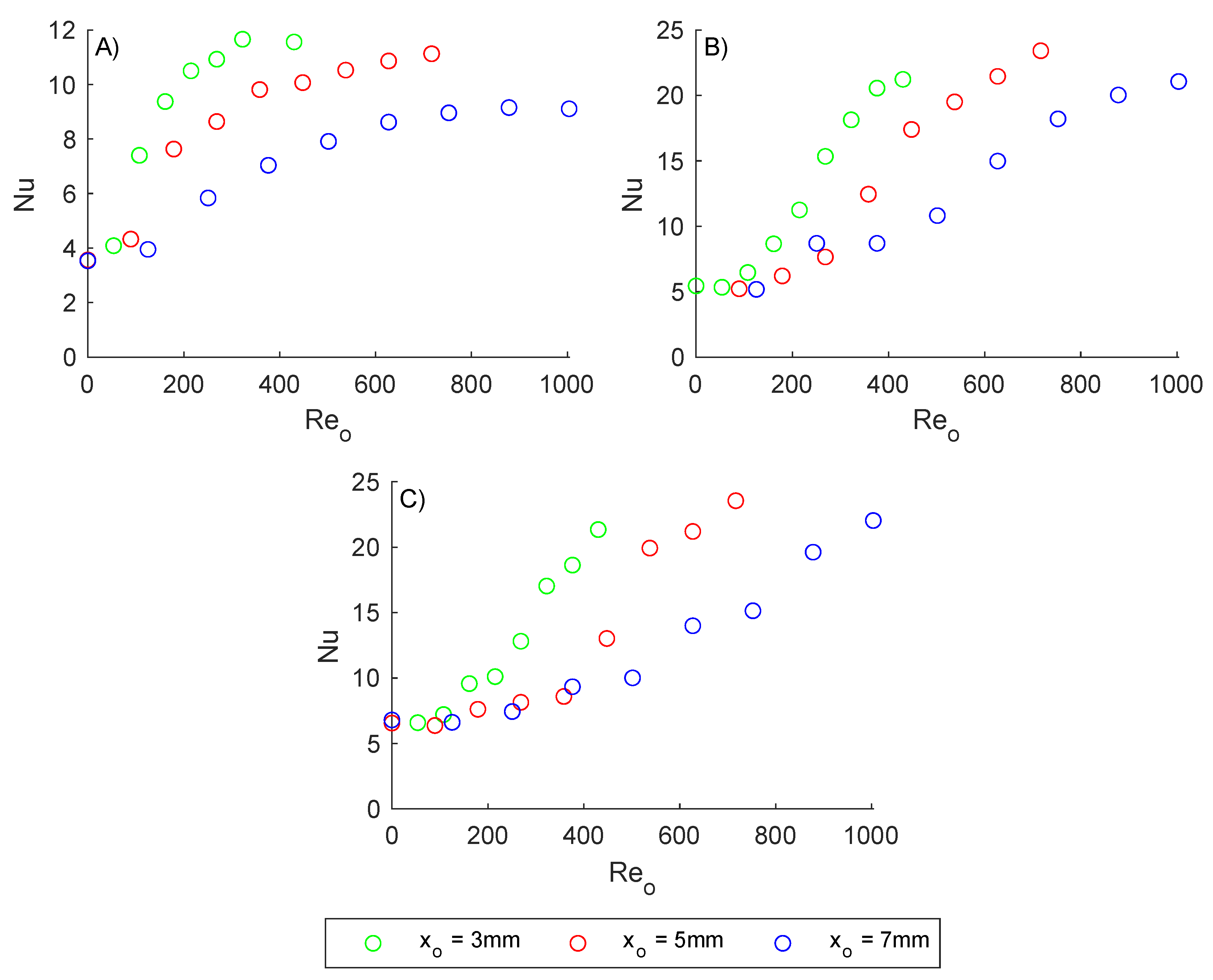
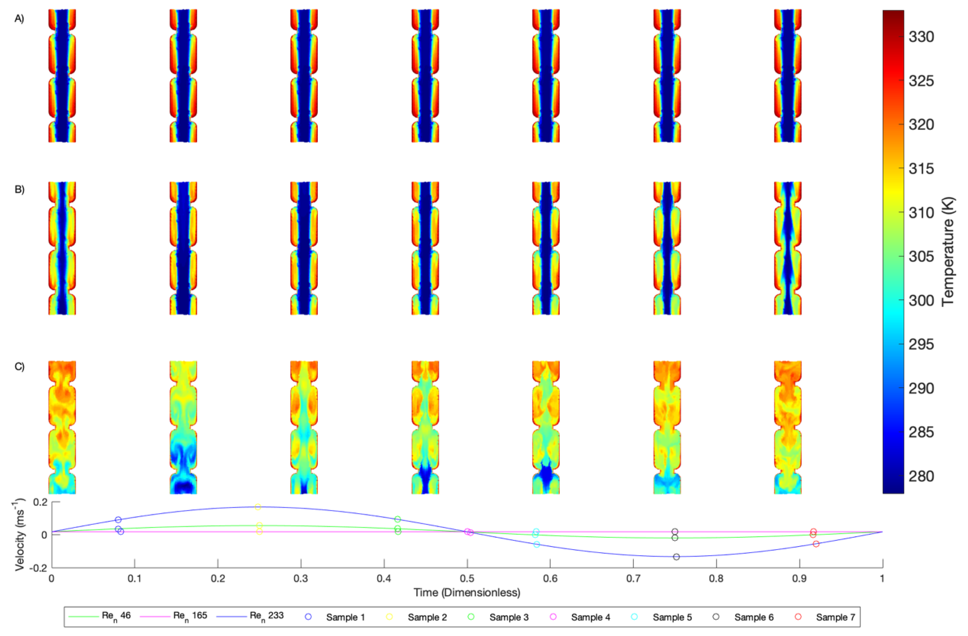
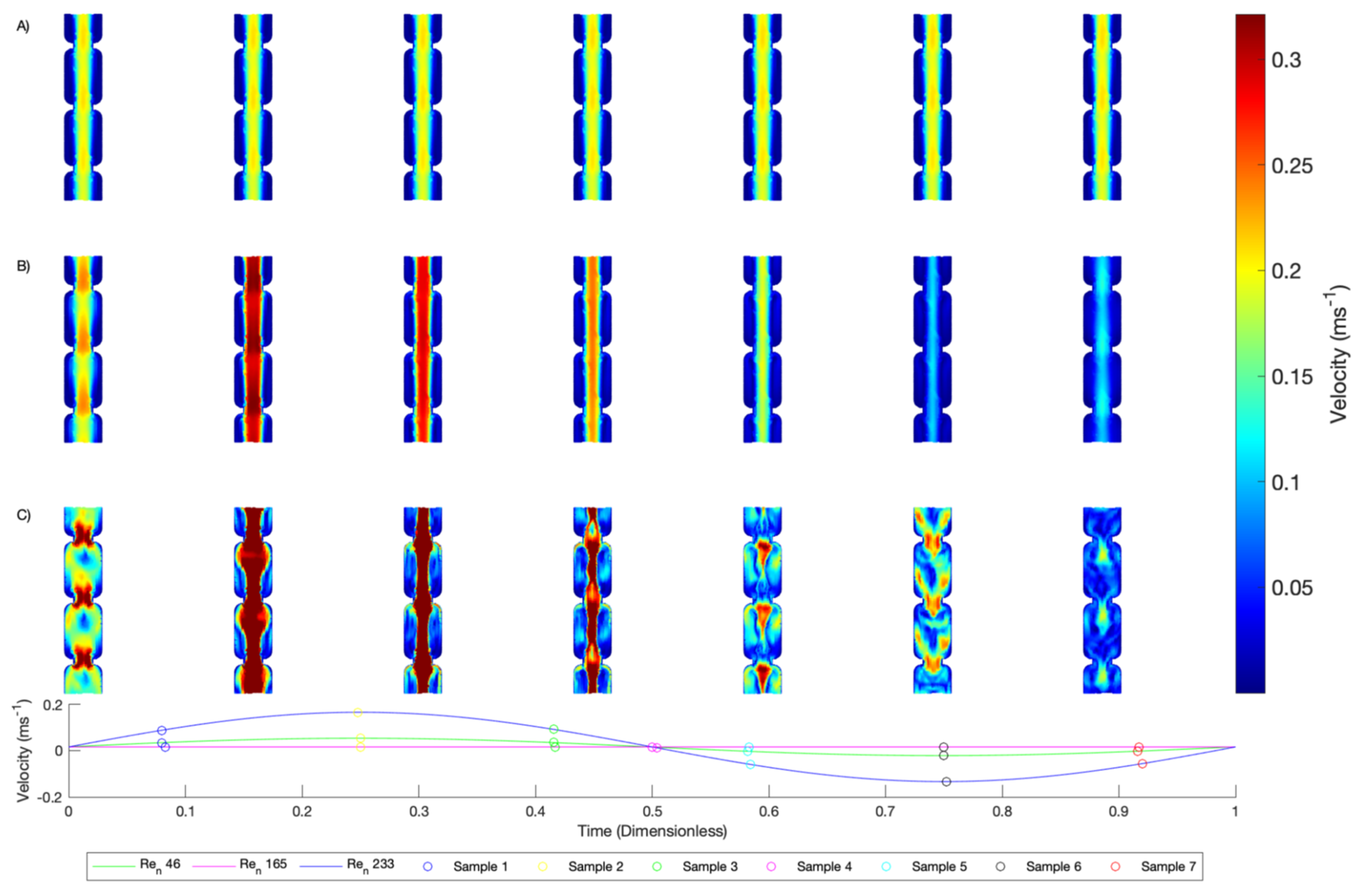
3.2. Heat Transfer Enhancement

To demonstrate the impact that the flow condition has on the heat transfer performance of the channels, the channel Nusselt number (Nu) was plotted against ${Re}_o$, as shown in Figure 5. The data are grouped by ${Re}_n$, 46 (A), 165 (B) and 233 (C), and the data for each oscillation amplitude are compared to demonstrate the effect that $x_o$ has on Nu. The oscillation frequency range was 0–8 Hz.

Figure 5 shows that for all net-flow conditions there is a clear enhancement in Nu with ${Re}_o$. For the net-flow condition ${Re}_n$ = 46, the maximum Nu enhancement is 227%, for ${Re}_n$ = 165 the maximum Nu enhancement is 348% and for a ${Re}_n$ of 233 the maximum Nu enhancement is 259%, compared to steady flow. Figure 5 also demonstrates the increase of Nu with ${Re}_n$, which indicates that the net-flow rate also has a significant impact on Nu, even under relatively intense oscillatory flows. Similar behaviours and levels of heat transfer enhancement have been observed previously in larger scale systems [19,34,35], which indicates conservation of the enhancement effect when scaling the process down to mini-scale.

The results also indicate there is a favourable effect of the lowering of $x_o$, with $x_o$ = 3 mm showing the steepest increase in Nu for all values of constant ${Re}_n$ and ${Re}_o$. This is likely due to channelling effects caused by the higher oscillation amplitudes “pushing” the flow beyond the gate baffles, which prevents effective flow separation and expansion within the spaces between the baffles. These channelling effects have also been observed when studying OBFs at larger scale when investigating mixing enhancement [36].

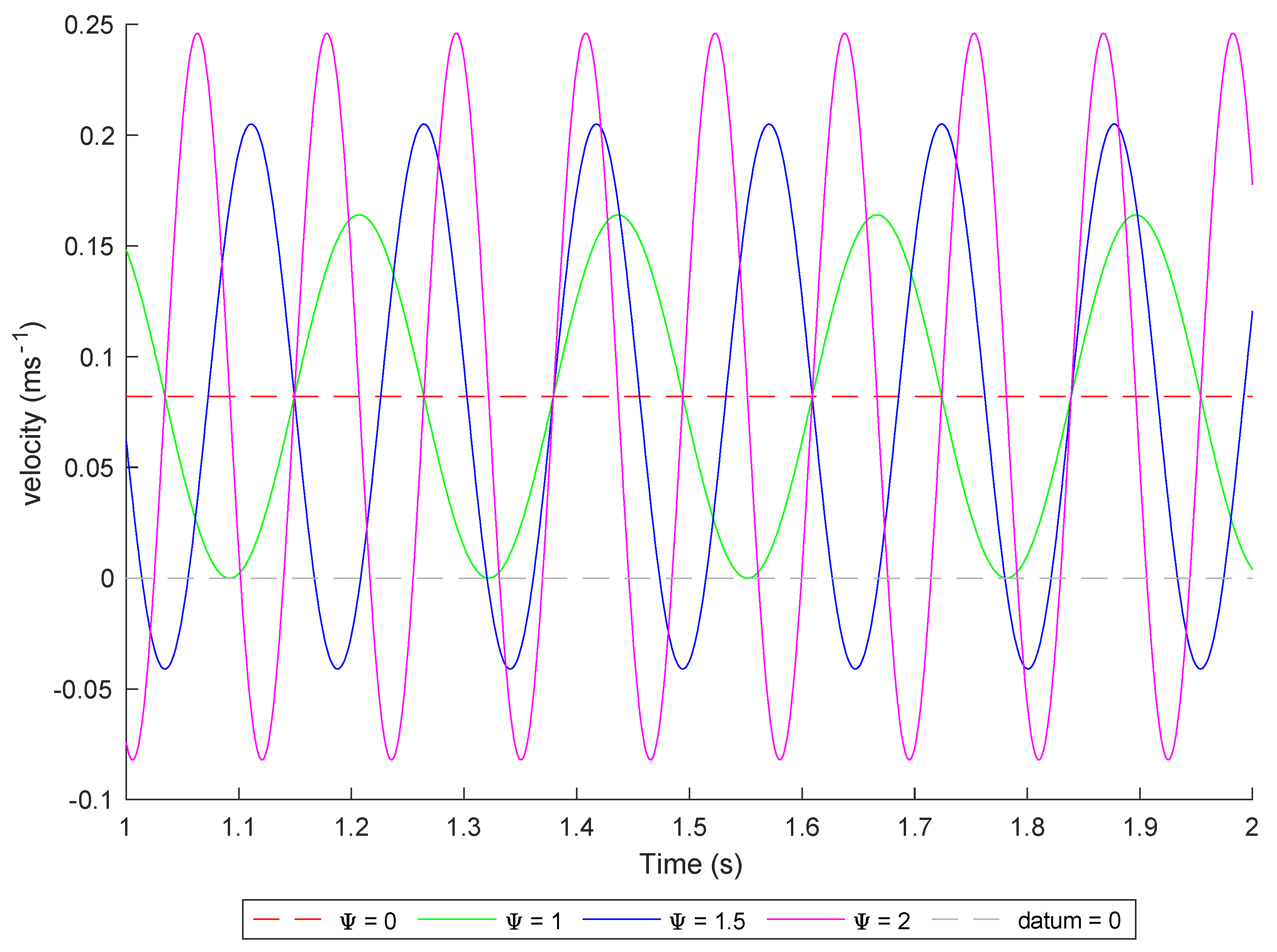
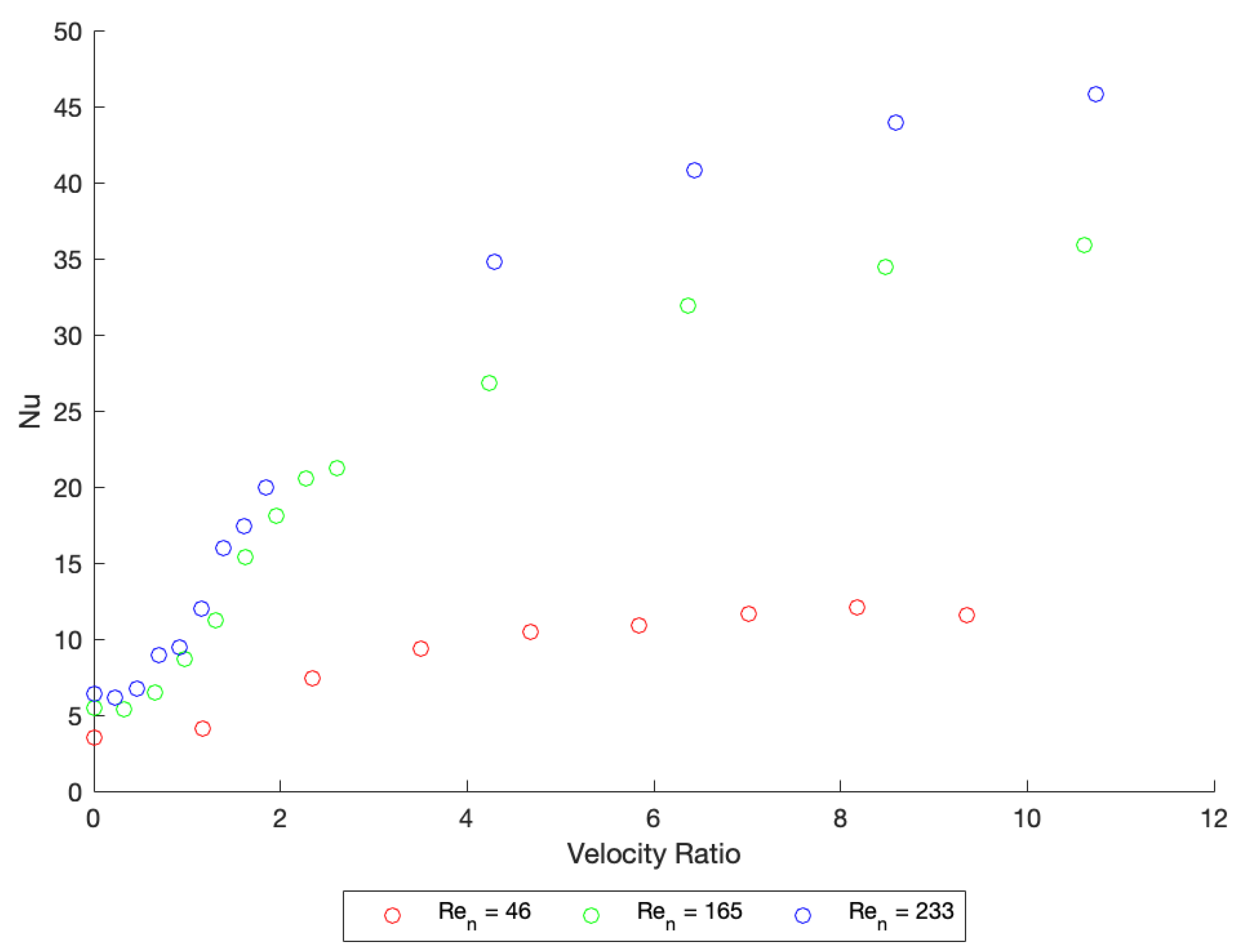
3.3. Effect of Velocity Ratio

At all net-flow rates, the enhancement in Nu is minimal in the lower range of ${Re}_o$. This effect implies that the velocity ratio (Equation (7)) is integral to Nu enhancement; a minimum $\mathsf{\Psi }$ is required for the onset of Nu enhancement. Furthermore, the results for a ${Re}_n$ of 46 show an apparent plateau in Nu at higher values of ${Re}_o$ (Figure 5A), indicating that there is an optimal value of $\mathsf{\Psi }$ required to reach maximum Nu enhancement. To investigate the effect further, $x_o$ was held constant at 3 mm, and higher oscillation frequencies (up to 46 Hz) were investigated so that a $\mathsf{\Psi }$ range of 0 to 10 could be analysed for ${Re}_n$ values of 46, 165 and 233. The results of this analysis are displayed in Figure 6.

Figure 6 confirms that $\mathsf{\Psi }$ has a significant effect on Nu enhancement. Significant Nu enhancement is not observed until $\mathsf{\Psi }$ increases beyond ~1. Beyond this value, the rise in Nu is significant and steep until beginning to level off at $\mathsf{\Psi }$ > ~4. As can be observed in Figure 3, at $\mathsf{\Psi }$ > 1 flow reversal is achieved on the downwards stroke of the oscillation. This facilitates vortex formation and flow separation around the baffles at both the forward and backward stroke, causing a significant enhancement in the mixing and therefore an enhancement in convective heat transfer within the single channel. The plateau in Nu at higher velocity ratios most likely indicates that some mixing limit has been achieved. This effect has previously been observed in heat transfer studies using OBFs for chemical reaction engineering [37].

To observe the effect that $\mathsf{\Psi }$ has on the flow patterns, the flow condition with the ${Re}_n$ of 165 was selected and the oscillation frequencies of 0 Hz, 2 Hz and 8 Hz analysed (Figure 6). These three flow conditions represent the data points in Figure 6 associated with the ${Re}_n$ of 165 and velocity ratios of 0, 0.33 and 2.6, which returned Nu values of 5.4, 6.5 and 21.2, respectively. Temperature contours obtained from the central plane of the test section (Figure 1) are shown for these conditions in Figure 7 and velocity contours in Figure 8.

Figure 7A represents the flow patterns for steady flow and shows areas of high temperature close to the walls of the channel, between the baffles ($\mathsf{\Psi }$ = 0). These areas represent dead zones in the fluid domain. Similar plots are shown for the case of $\mathsf{\Psi }$ = 0.65, where the oscillatory flow effect is not large enough to promote flow separation on either the forward or reverse stroke of the fluid oscillation (Figure 7B). In these two instances, channelling is observed in the centre of the fluid domain, caused by the net-flow velocity being dominant over the flow oscillations. The dead zones behind the baffles are completely eliminated when $\mathsf{\Psi }$ increases to 2.6 (Figure 7C) and the areas of high temperature are less apparent compared to Figure 7A,B. This is a clear effect of the mixing caused by the complete flow reversal at the higher value of $\mathsf{\Psi }$ and is an indication of flow separation around the baffles. This effect is investigated by plotting the fluid velocity contours over the same oscillation period. These data are presented in Figure 8.

The velocity profiles in Figure 8A,B show clear channelling between the gate baffles and dead zones in the baffle wakes, mirroring the results shown in Figure 7.

Figure 8C demonstrates the intense mixing achieved in the baffle cavities across the oscillation cycle. Channelling effects are only observable on the downward stroke as the fluid velocity approaches the value of net-flow velocity. The flow patterns throughout the rest of the oscillation cycle show clear vortex generation into the cavities, providing intense mixing of the bulk flow fluid towards the walls. This explains the large convective heat transfer enhancement observed in Figure 6.

To further demonstrate the impact of the flow oscillations, Figure 9 shows Nu as a function of the total Reynolds number, ${Re}_T$, (Equation (8)), which considers the maximum forward velocity of the combined flow (oscillatory flow and net flow combined). The data for oscillatory flow is compared to steady flow up to a ${Re}_n$ of 600 in order to consider how much of the enhancement was due to the unsteady nature of the flow and how much can be considered a “combined velocity” effect.

Figure 9 shows that for a lower velocity ratio the oscillatory flow data roughly follow the trend of steady flow at an equivalent Reynolds number. Hence, the heat transfer enhancement at a low velocity ratio, which is relatively modest, can be attributed to a “summed velocity” effect, i.e., the enhancement is only caused by an increase in the flow velocity during the upstroke of the oscillation cycle and this level of Nu could be replicated by instead increasing the net-flow rate of a steady flow.

At a higher velocity ratio ($\mathsf{\Psi }$ > ~1.2) more significant enhancement is observed, and the Nu achieved is considerably higher than what would be achieved by simply increasing the net flow (pink line Figure 9). For example, at a ${Re}_T$ of 280, ${Re}_n$ 46 (corresponding to a ${Re}_o$ of 200, $f$ of 4 Hz and $x_o$ of 3 mm), a Nusselt number is achieved which would require a ${Re}_n$ of around 430 for the steady flow equivalent. This highlights that OBFs can be used to achieve high heat transfer coefficients at lower net-flow rates. This effect could be used to facilitate significant heat transfer enhancement in parallel channels without needing to increase the mass flow through the heat sink, which may in turn have applications in recovering reusable (i.e., higher temperature) waste heat from electronics.

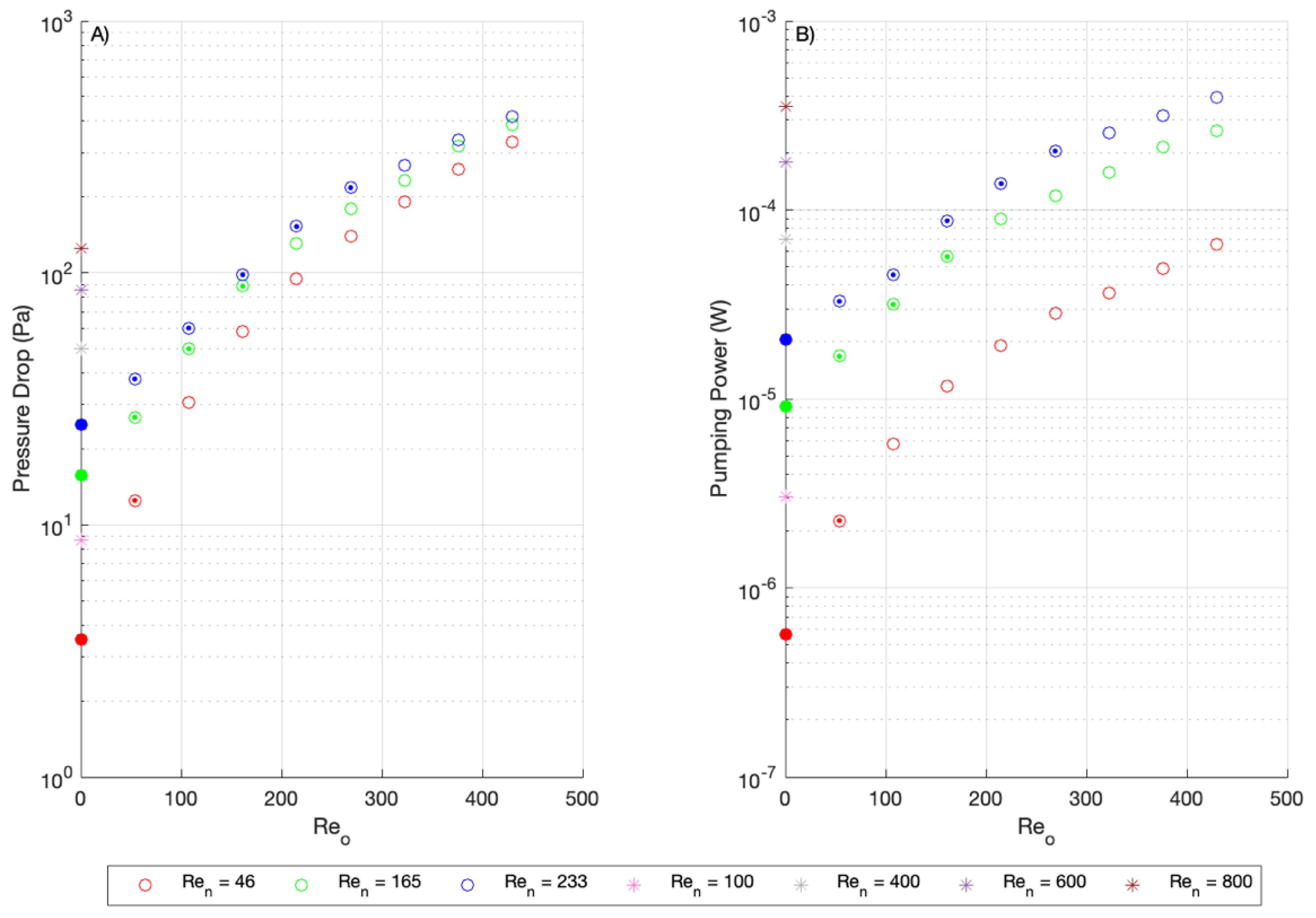
3.4. Power Requirements for Oscillatory Flow

The pressure drop values between chambers 6 and 3 (Figure 1) were recorded and are displayed in Figure 10. These values were recorded for all three values of ${Re}_n$ investigated, as well as for elevated Reynolds numbers recorded for steady flow values (100, 400, 600, and 800), and are displayed in Figure 10A. The pumping power required for the flow conditions was calculated as described by Mackley et al. [19], using Equations (14)–(16). The results of this analysis are presented in Figure 10B.

Figure 10A shows that little difference is observed in pressure drop between the datapoints for ${Re}_n$ 46, 165 and 233, highlighting that the oscillatory flow component is dominant. There is more distinction between the net-flow rate data for pumping power (Figure 10B) due to the differences in the net volumetric flow rate for each case. However, as with the pressure drop data, the increase in ${Re}_o$ dominates the effect on the required pumping power.

When analysing how the pressure drop and required pumping power increases with ${Re}_o$, the initial increase is rapid when oscillations are first initiated, but then drops off as oscillations increase in frequency. At larger scale [19,38], similar phenomena have been observed with the reason attributed to energy recovery on the oscillation downstroke as flow vortices unwind. This is not observed at lower values of $\mathsf{\Psi }$ as the oscillation intensity is not sufficient to cause vortex formation. Hence, the increase in the power requirement levels off at higher values of ${Re}_o$.

The impact of the pumping power on thermal performance was investigated by plotting the pumping power against the thermal resistance of the channels. This data is displayed in Figure 11.

The data presented in Figure 11 lie in two distinct regions governed by the velocity ratio. The higher thermal resistance is associated with the flows that are under the low velocity ratio conditions characterised by $\mathsf{\Psi }$ less than or equal to 1. This occurs for all ${Re}_n$ values tested for the oscillatory flow conditions, but when steady flow conditions are investigated, ${Re}_n$ = 400 (149 mm s⁻¹) is the maximum net-flow Reynolds number analysed that lies in the low-velocity ratio region. When ${Re}_n$ exceeds 400, the datapoints for pumping power vs. thermal resistance lie in the high velocity ratio region.

Figure 11 shows that at lower values of velocity ratio ($\mathsf{\Psi }$< 1.2) (green trend line), the data for oscillatory flow roughly tracks the data for steady flow. This again implies that there is a “summed velocity” effect at the low velocity ratio, for both pumping power and thermal resistance. The data obtained when the velocity ratio was greater than 1.2 falls in a distinctly different region (red trend line). Here, low thermal resistance can be attained for relatively low pumping power and there is a clear favouring of a high velocity ratio and low ${Re}_n$ flow conditions compared to operating at elevated steady flowrates.

Two data points were chosen for further analysis, as highlighted by the red circles in Figure 11. The data point representing ${Re}_n$ 165 with an oscillation frequency of 2 Hz, $\mathsf{\Psi }$ of 0.65, has a pumping power requirement of ~3.3 × 10⁻⁵ W and a thermal resistance of 2.1 K·W⁻¹. The datapoint for a ${Re}_n$ of 46, with an oscillation frequency of 5 Hz and $\mathsf{\Psi }$ of 5.84, shows the pumping power is also ~3.3 × 10⁻⁵ W but the thermal resistance is 1.25 K W⁻¹. Hence, for the same pumping power the convective thermal resistance reduces by around 40%, between the two cases.

To visualise the hydrodynamics of the flows associated with these two data points, velocity and temperature contours are displayed in Figure 12 and Figure 13, respectively. This contour data is split into (A) ${Re}_n$ 46 with an oscillation frequency of 6 Hz and (B) ${Re}_n$ 165 with an oscillation frequency of 2 Hz.

The velocity contours in Figure 12A show a clear vortex formation and relatively intense mixing caused by the more intense oscillations. Figure 12B displays the velocity profiles for the ${Re}_n$ 165 flow conditions and an oscillation frequency of 2 Hz, with the velocity profile showing no evidence of vortex formation behind the baffles and a clear channelling of the flow. This provides an explanation for the reduction in thermal resistance observed in Figure 11 when the ${Re}_n$ drops from 165 to 46, but both cases require the same pumping power to achieve the same thermal performance.

To visualise the effect of the lower thermal resistance between the two flow conditions, the temperature contours are displayed in Figure 13.

The effect of the vortex formation as observed in Figure 12A on the temperature profile can clearly be seen in Figure 13A. Because the fluid within the baffle cavities is well mixed, there is a consistent temperature profile in the radial direction, which is in stark contrast to the temperature contours displayed in Figure 13B. The lower velocity ratio case shown in Figure 13B shows clear channelling of the bulk flow and dead zones behind the baffles.

This is a clear visualisation of the effect that the value of $\mathsf{\Psi }$ has on the fluid mixing and convective heat transport. To the authors’ knowledge, the effect of $\mathsf{\Psi }$ has not been visualised in this way previously; Figure 11 clearly demonstrates two distinct regions of thermal resistance, governed by the value of $\mathsf{\Psi }$. Figure 11, Figure 12 and Figure 13 clearly demonstrate the enhancement caused by the imposition of flow oscillations to the system; a flow with a higher net-flow rate but less severe oscillations will require the same pumping duty as a flow with a lower net-flow velocity but more vigorous oscillations, the result being that the latter has enhanced convective transport.

The same effect can be observed for the flow conditions with a ${Re}_n$ of 46 and an oscillation frequency of 4 Hz compared to the steady flow case with a ${Re}_n$ of 233. For each case, the pumping power is approx. 3.3 × 10⁻⁵ W; however, there is a 40% reduction in thermal resistance for the ${Re}_n$ 46 conditions compared to the steady-flow ${Re}_n$ 233 conditions. This results in an increase of 65% in Nu for the ${Re}_n$ 46 flow conditions compared to the steady flow conditions with a ${Re}_n$ of 233 (Figure 9), with the same pumping duty requirements.

More generally, it can be observed that for a pumping power of 10⁻⁶ to 10⁻⁴ W the thermal resistance for cases where $\mathsf{\Psi }$ > 1 will always outperform that of when $\mathsf{\Psi }$ ≤ 1, showing a thermal resistance reduction of 30–40% for a similar pumping power. This represents the useful operating window of using oscillatory flows for this channel containing gate baffles. Based on these results, there is a hydrodynamic case for improving convective performance via oscillating the flow rather than simply increasing the flow rate. This concept may also open more opportunities for waste heat recovery from electronic components (for example in data centres). Achieving high heat transfer coefficients at lower flow rates may provide opportunities for high flux cooling whilst also recovering water at a useful temperature.

These results are a clear demonstration of the benefit of scaling down OBFs, although it must be acknowledged that these results are theoretical and further work will be required to validate these results. The concept demonstrated in this study may be applicable to heat sinks containing parallel channels where a higher net-flow rate is distributed between each channel, but issues of flow-distribution would need to be addressed [3,4,5].

4. Conclusions

This numerical study is the first attempt in the literature to characterise the heat transfer performance of an oscillatory baffled flow at the mini-scale with a view to utilising OBFs for the cooling of power electronics. The geometry consisted of 2 × 5 mm channels ($D_h$ = 2.8 mm) with gate baffles with a 50% open area providing flow disturbance. The net-flow Reynolds number for the flows ranged from 46 to 233, the oscillation amplitude ranged from 3 mm to 7 mm and the frequency was varied from 0 Hz (steady flow) to 8 Hz. The study also considered higher frequencies to compare the effect of the velocity ratio on the heat transfer performance of the channels. Within the range of frequency investigated, the maximum heat transfer enhancement was obtained when the oscillation amplitude was 3 mm.

The maximum enhancement in the Nusselt number was 227% for a net-flow Re of 46, 330% for ${Re}_n$ 165 and 259% for ${Re}_n$ 233. The level of heat transfer enhancement was minimal for velocity ratios < 1.2, but enhancement sharply increased to a maximum as $\mathsf{\Psi }$ increased. At a velocity ratio of 10 the Nu reached an approximate plateau, suggesting that a mixing limit had been reached under these flow conditions.

Contours of temperature and velocity were explored to further investigate the cause of the heat transfer enhancement. At a velocity ratio of less than 1.2, little flow detachment was observed, and significant dead zones persisted in the baffle wakes. As the velocity ratio increased beyond 1, the baffle cavities became extremely well mixed, which facilitated high rates of convective heat transport.

Analysis of the pressure drop and pumping power identified the useful operating range for oscillatory flows within the confines of this study. Generally, oscillatory flow cases showed a decrease in thermal resistance of 30–40% for constant pumping power compared to steady flow cases, within the identified operating window (velocity ratio greater than 1).

The results in this paper have shown that oscillatory baffled flows could provide a step change in liquid cooling performance in mini-channel heat sinks, with Nusselt number enhancements which go beyond those reported for passive methods. However, there is a need to extend this study via experimentation for the purposes of validation, geometric optimisation and practical implementation.

References

1. Zhang, Z.; Wang, X.; Yan, Y. A review of the state-of-the-art in electronic cooling. e-Prime-Adv. Electr. Eng. Electron. Energy 2021, 1, 100009. [Google Scholar] [CrossRef]
2. Moore, S.K. The Transistor of 2047: What will the device be like on its 100th anniversary? IEEE Spectr. 2022, 59, 38–39. [Google Scholar] [CrossRef]
3. Qu, W.; Mudawar, I. Analysis of three-dimensional heat transfer in micro-channel heat sinks. Int. J. Heat Mass Transf. 2002, 45, 3973–3985. [Google Scholar] [CrossRef]
4. Marzougui, M.; Hammami, M.; Ben Maad, R. Experimental study on thermal performance of heat sinks: The effect of hydraulic diameter and geometric shape. Heat Mass Transf. 2015, 52, 2091–2100. [Google Scholar] [CrossRef]
5. Liu, X.; Yu, J. Numerical study on performances of mini-channel heat sinks with non-uniform inlets. Appl. Therm. Eng. 2016, 93, 856–864. [Google Scholar] [CrossRef]
6. Wei, M.; Boutin, G.; Fan, Y.; Luo, L. Numerical and experimental investigation on the realization of target flow distribution among parallel mini-channels. Chem. Eng. Res. Des. 2016, 113, 74–84. [Google Scholar] [CrossRef]
7. Anbumeenakshi, C.; Thansekhar, M. Experimental investigation of header shape and inlet configuration on flow maldistribution in microchannel. Exp. Therm. Fluid Sci. 2016, 75, 156–161. [Google Scholar] [CrossRef]
8. Mu, Y.-T.; Chen, L.; He, Y.-L.; Tao, W.-Q. Numerical study on temperature uniformity in a novel mini-channel heat sink with different flow field configurations. Int. J. Heat Mass Transf. 2015, 85, 147–157. [Google Scholar] [CrossRef]
9. Xu, M.; Lu, H.; Gong, L.; Chai, J.C.; Duan, X. Parametric numerical study of the flow and heat transfer in microchannel with dimples. Int. Commun. Heat Mass Transf. 2016, 76, 348–357. [Google Scholar] [CrossRef]
10. Khoshvaght-Aliabadi, M.; Sahamiyan, M.; Hesampour, M.; Sartipzadeh, O. Experimental study on cooling performance of sinusoidal–wavy minichannel heat sink. Appl. Therm. Eng. 2016, 92, 50–61. [Google Scholar] [CrossRef]
11. Jadhav, S.V.; Kale, S.M.; Kashid, D.T.; Kakade, S.S.; Gavali, S.R.; Shinde, S.D. Performance Analysis of Heat Sink with Different Microchannel Orientations. In Techno-Societal 2018; Springer International Publishing: Cham, Switzerland, 2020. [Google Scholar]
12. Duangthongsuk, W.; Wongwises, S. A comparison of the thermal and hydraulic performances between miniature pin fin heat sink and microchannel heat sink with zigzag flow channel together with using nanofluids. Heat Mass Transf. 2018, 54, 3265–3274. [Google Scholar] [CrossRef]
13. Scott, A.W. Cooling of Electronic Equipment; John Wiley & Sons: Hoboken, NJ, USA, 1974. [Google Scholar]
14. Meybodi, M.K.; Daryasafar, A.; Koochi, M.M.; Moghadasi, J.; Meybodi, R.B.; Ghahfarokhi, A.K. A novel correlation approach for viscosity prediction of water based nanofluids of Al2O3, TiO2, SiO2 and CuO. J. Taiwan Inst. Chem. Eng. 2016, 58, 19–27. [Google Scholar] [CrossRef]
15. Nada, S.A.; El-Zoheiry, R.M.; Elsharnoby, M.; Osman, O.S. Enhancing the thermal performance of different flow configuration minichannel heat sink using Al2O3 and CuO-water nanofluids for electronic cooling: An experimental assessment. Int. J. Therm. Sci. 2022, 181, 107767. [Google Scholar] [CrossRef]
16. Alkasmoul, F.S.; Al-Asadi, M.T.; Myers, T.G.; Thompson, H.M.; Wilson, M.C.T. A practical evaluation of the performance of Al2O3-water, TiO2-water and CuO-water nanofluids for convective cooling. Int. J. Heat Mass Transf. 2018, 126, 639–651. [Google Scholar] [CrossRef]
17. Al-Neama, A.F.; Kapur, N.; Summers, J.; Thompson, H.M. Thermal management of GaN HEMT devices using serpentine minichannel heat sinks. Appl. Therm. Eng. 2018, 140, 622–636. [Google Scholar] [CrossRef]
18. Al-Neama, A.F.; Khatir, Z.; Kapur, N.; Summers, J.; Thompson, H.M. An experimental and numerical investigation of chevron fin structures in serpentine minichannel heat sinks. Int. J. Heat Mass Transf. 2018, 120, 1213–1228. [Google Scholar] [CrossRef]
19. Mackley, M.; Stonestreet, P. Heat transfer and associated energy dissipation for oscillatory flow in baffled tubes. Chem. Eng. Sci. 1995, 50, 2211–2224. [Google Scholar] [CrossRef]
20. Ahmed, S.M.; Law, R.; Phan, A.N.; Harvey, A.P. Thermal performance of meso-scale oscillatory baffled reactors. Chem. Eng. Process.-Process. Intensif. 2018, 132, 25–33. [Google Scholar] [CrossRef]
21. Law, R.; Ahmed, S.M.; Tang, N.; Phan, A.N.; Harvey, A.P. Development of a more robust correlation for predicting heat transfer performance in oscillatory baffled reactors. Chem. Eng. Process.-Process. Intensif. 2018, 125, 133–138. [Google Scholar] [CrossRef]
22. McDonough, J.; Ahmed, S.; Phan, A.; Harvey, A. A study of the flow structures generated by oscillating flows in a helical baffled tube. Chem. Eng. Sci. 2017, 171, 160–178. [Google Scholar] [CrossRef]
23. Phan, A.N.; Harvey, A. Development and evaluation of novel designs of continuous mesoscale oscillatory baffled reactors. Chem. Eng. J. 2010, 159, 212–219. [Google Scholar] [CrossRef]
24. Stonestreet, P.; Harvey, A. A Mixing-Based Design Methodology for Continuous Oscillatory Flow Reactors. Chem. Eng. Res. Des. 2002, 80, 31–44. [Google Scholar] [CrossRef]
25. Phan, A.N.; Harvey, A.P. Characterisation of mesoscale oscillatory helical baffled reactor—Experimental approach. Chem. Eng. J. 2012, 180, 229–236. [Google Scholar] [CrossRef]
26. Muñoz-Cámara, J.; Crespí-Llorens, D.; Solano, J.; Vicente, P. Effect of three-orifice baffles orientation on the flow and thermal–hydraulic performance: Experimental analysis for net and oscillatory flows. Appl. Therm. Eng. 2024, 236, 121566. [Google Scholar] [CrossRef]
27. Gonzalez-Juarez, D.; Herrero-Martin, R.; Solano, J.P. Enhanced heat transfer and power dissipation in oscillatory-flow tubes with circular-orifice baffles: A numerical study. Appl. Therm. Eng. 2018, 141, 494–502. [Google Scholar] [CrossRef]
28. Solano, J.; Herrero, R.; Espín, S.; Phan, A.; Harvey, A. Numerical study of the flow pattern and heat transfer enhancement in oscillatory baffled reactors with helical coil inserts. Chem. Eng. Res. Des. 2012, 90, 732–742. [Google Scholar] [CrossRef]
29. Versteeg, H.K.; Malalasekera, W. An Introduction to Computational Fluid Dynamics: The Finite Volume Method; Pearson Education Limited: London, UK, 2007. [Google Scholar]
30. McDonough, J.; Ahmed, S.; Phan, A.; Harvey, A. The development of helical vortex pairs in oscillatory flows—A numerical and experimental study. Chem. Eng. Process.-Process. Intensif. 2019, 143, 107588. [Google Scholar] [CrossRef]
31. Nogueira, X.; Taylor, B.J.; Gomez, H.; Colominas, I.; Mackley, M.R. Experimental and computational modeling of oscillatory flow within a baffled tube containing periodic-tri-orifice baffle geometries. Comput. Chem. Eng. 2013, 49, 107588. [Google Scholar] [CrossRef]
32. Wang, J.; Li, Y.; Liu, X.; Shen, C.; Zhang, H.; Xiong, K. Recent active thermal management technologies for the development of energy-optimized aerospace vehicles in China. Chin. J. Aeronaut. 2020, 34, 1–27. [Google Scholar] [CrossRef]
33. McDonough, J.; Oates, M.; Law, R.; Harvey, A. Micromixing in oscillatory baffled flows. Chem. Eng. J. 2018, 361, 508–518. [Google Scholar] [CrossRef]
34. Munoz-Camara, J.; Crespi-Llorens, D.; Solano, J.P.; Vicente, P.G. Experimental analysis of flow pattern and heat transfer in circular-orifice baffled tubes. Int. J. Heat Mass Transf. 2020, 147, 118914. [Google Scholar] [CrossRef]
35. Muñoz-Cámara, J.; Crespí-Llorens, D.; Solano, J.; Vicente, P. Baffled tubes with superimposed oscillatory flow: Experimental study of the fluid mixing and heat transfer at low net Reynolds numbers. Exp. Therm. Fluid Sci. 2020, 123, 110324. [Google Scholar] [CrossRef]
36. Phan, A.N.; Harvey, A.P.; Rawcliffe, M. Continuous screening of base-catalysed biodiesel production using new designs of mesoscale oscillatory baffled reactors. Fuel Process. Technol. 2011, 92, 1560–1567. [Google Scholar] [CrossRef]
37. Howes, T.; Mackley, M.; Roberts, E. The simulation of chaotic mixing and dispersion for periodic flows in baffled channels. Chem. Eng. Sci. 1991, 46, 1669–1677. [Google Scholar] [CrossRef]
38. Muñoz-Cámara, J.; Solano, J.; Pérez-García, J. Non-dimensional analysis of experimental pressure drop and energy dissipation measurements in Oscillatory Baffled Reactors. Chem. Eng. Sci. 2022, 262, 118030. [Google Scholar] [CrossRef]
Figure 1. A 60 mm long baffled channel. The inlet and outlet are located normal to the x plane, and all other walls were given a constant wall temperature of 60 °C.
Energies 17 02459 g001
Figure 2. The fluid body model, discretised into finite elements for the CFD investigation, cross-section cut at the centre of chamber 4.
Energies 17 02459 g002
Figure 3. Velocity profiles of a fluid flow with varying velocity ratio. Oscillation amplitude was kept constant at 3 mm, and oscillation frequency altered to achieve Ψ = 1, Ψ = 1.5 and Ψ = 2.
Energies 17 02459 g003
Figure 4. Results of the grid independence study for the calculated value of Nu plotted against the associated mesh number. (A) shows how Nusselt number varies between the meshes; (B) shows how pressure drop varies between the meshes.
Energies 17 02459 g004
Figure 5. The effect of increasing R e o for a frequency range of 0 Hz to 8 Hz. (A) R e n constant at 46, (B) R e n constant at 165, (C) R e n constant at 233.
Energies 17 02459 g005
Figure 6. Nusselt number plotted against Ψ with the oscillation amplitude held constant at 3 mm. Frequency for each case was modified in accordance with Equations (6) and (7).
Energies 17 02459 g006
Figure 7. Effect that increasing R e o has on the temperature contours while R e n held constant at 165. (A) Ψ of 0, (B) Ψ of 0.65 and (C) Ψ of 2.6.
Energies 17 02459 g007
Figure 8. Effect that increasing R e o has on the velocity contours while R e n held constant at 165. (A) Ψ of 0, (B) Ψ of 0.65 and (C) Ψ of 2.6.
Energies 17 02459 g008
Figure 9. Nusselt number plotted against the total Reynolds number. Oscillation amplitude held constant at 3 mm. Fully-filled data points represent steady flow data ( R e o = 0) and partially-filled data points represent Ψ < 1.2 .
Energies 17 02459 g009
Figure 10. (A). Pressure drop plotted v. R e o (B). Pumping Power v. R e o for 3 mm oscillation amplitude. The fully-filled markers indicate steady flow conditions ( R e o = 0), and the partially-filled markers indicate Ψ < 1.2 . Also shown is data for steady flow only at higher flow rates, indicated by stars.
Energies 17 02459 g010
Figure 11. Pumping power vs. resistance for 3 mm amplitude oscillations. Red line fits data points for velocity ratio > 1.2, green line for velocity ratio < 1.2. The solid filled markers indicate steady flow conditions ( R e o = 0), and the partially filled markers indicate data with a Ψ < 1.2.
Energies 17 02459 g011
Figure 12. Comparing velocity contours at different stages of an oscillation cycle for (A) R e n 46 with an oscillation frequency of 6 Hz, Ψ = 7.01; (B) R e n 165 with an oscillation frequency of 2 Hz, Ψ = 0.65.
Energies 17 02459 g012
Figure 13. Comparing temperature contours at different stages of an oscillation cycle for (A) R e n 46 with an oscillation frequency of 6 Hz, Ψ = 7.01; (B) R e n of 165 with an oscillation frequency of 2 Hz, Ψ = 0.65.
Energies 17 02459 g013