Abstract
Accurate quantification of uncertainty in solar photovoltaic (PV) generation forecasts is imperative for the efficient and reliable operation of the power grid. In this paper, a data-driven non-parametric probabilistic method based on the Naïve Bayes (NB) classification algorithm and Dempster–Shafer theory (DST) of evidence is proposed for day-ahead probabilistic PV power forecasting. This NB-DST method extends traditional deterministic solar PV forecasting methods by quantifying the uncertainty of their forecasts by estimating the cumulative distribution functions (CDFs) of their forecast errors and forecast variables. The statistical performance of this method is compared with the analog ensemble method and the persistence ensemble method under three different weather conditions using real-world data. The study results reveal that the proposed NB-DST method coupled with an artificial neural network model outperforms the other methods in that its estimated CDFs have lower spread, higher reliability, and sharper probabilistic forecasts with better accuracy.
1. Introduction
Solar photovoltaic (PV) generation has been penetrating the power grid at an accelerating speed over the past decade as the world moves toward a more sustainable energy grid. Integrating a large number of solar PV power plants into the existing conventional grid presents significant challenges because solar PV generation is not dispatchable and is often treated as a form of negative load in power grid operations. To efficiently maintain the balance between generation and load in the power grid, both load and solar PV generation need to be forecasted. These forecasts enable the proactive scheduling of dispatchable generation resources, allowing for the management of power ramping and the timely allocation of generation reserves to address power uncertainty [1,2]. Moreover, solar PV power forecasting plays a significant role in predicting energy market imbalances and optimizing bid scheduling [3].
To support the bidding strategy and operation of a day-ahead electric power market, many data-driven forecasting methods have been developed to forecast solar PV generation. Typically, these day-ahead forecasting methods have forecast horizons between 24 and 48 h, with a lead time of 24 h. In other words, the first instance of the forecast is 24 h ahead in the future relative to the current time [4]. Because of the large lead time, all forecasting methods inherently exhibit some levels of forecast errors that cannot be overlooked. Based on how they handle the uncertainty associated with the forecast errors, the forecasting methods can be broadly categorized into deterministic and probabilistic approaches. While deterministic methods provide a single-value forecast without quantifying forecast uncertainty, probabilistic methods quantify forecast uncertainty by estimating statistical properties of forecast variables, such as probability distributions and prediction intervals (PIs) [5].
Many deterministic methods have been developed to accurately forecast solar PV generation, gaining widespread acceptance in real-world applications [6,7,8,9,10]. Well-recognized forecasting methods include artificial neural networks (ANN) [11], recurrent neural networks (RNN) [12], long-short term memory (LSTM) [13], convolutional neural network (CNN) [14], and support vector regression (SVR) [15,16]. Deterministic forecasting methods excel at estimating the expected solar PV generation and are valuable for managing power ramping. Yet, they cannot be directly used to address the uncertainty associated with solar PV generation.
Many probabilistic methods have been developed to quantify the uncertainty inherent in solar PV forecasts. For instance, the persistence ensemble (PerEn) method assumes that the forecasted solar PV generation follows a Gaussian distribution [17] and subsequently estimates its mean and variance. Meanwhile, the ensemble learning method (ELM) [18] integrates various deterministic forecasting methods, including k-nearest neighbors (kNN), decision trees, gradient boosting, random forest, lasso, and ridge regression, to estimate forecast distributions. For deep learning, an improved deep ensemble method, CNN-BiLSTM, is proposed in [19] for probabilistic wind speed forecasting, where the outputs of the final CNN-BiLSTM layer are fitted to a Gaussian distribution to estimate the mean and variance of the wind speed. Quantile regression (QR), on the other hand, estimates the conditional quantiles of solar irradiance based on numerical weather prediction (NWP) data [20]. In addition, an analog ensemble (AnEn) method is developed by [21] and compared to QR and PerEn methods. The AnEn method requires a frozen meteorological model to identify forecast points in the training dataset most similar to the current forecast. Furthermore, Doubleday et al. propose combining several deterministic NWP model outputs using the Bayesian model averaging (BMA) technique to estimate forecast distributions [22]. In [23], Gaussian process regression (GPR) with specific kernel functions is applied to obtain prediction intervals of solar power forecast. This method tries to quantify the forecast uncertainty by fitting the forecast errors to a standard normal distribution. A sparse GPR method is proposed in [24] for probabilistic wind-gust forecasting by combining NWP data and on-site measurements. A variant of this method has shown promise for solar power forecasting of geographically sparse distributed solar plants [25]. The uncertainty quantified by probabilistic forecasting methods serves as a valuable guide for operators in booking appropriate generation reserves.
However, these probabilistic forecasting methods have certain limitations and challenges. For example, the AnEn, ELM, CNN-BiLSTM, and BMA rely on the assumption that a predefined family of probabilistic distributions can adequately characterize their forecasts. The GPR-based approaches, however, non-parametrically forecast the solar power generation but fit the forecast error to a standard normal distribution to quantify the uncertainty. As a result, discrepancies between actual and assumed distributions may lead to significant errors. In addition, both the ELM and BMA methods require forecast outputs from several NWP models, which is time-consuming and may introduce additional uncertainty due to variation across models. As such, these methods have not gained widespread adoption in practical applications.
To overcome the above-mentioned limitations inherent in existing probabilistic forecasting methods and leverage the widespread acceptance of deterministic forecasting methods, this paper proposes a data-driven non-parametric statistical method for day-ahead probabilistic forecasting of PV power [26]. First, the method estimates the probability of the forecast error falling into a certain interval using the Naïve Bayes (NB) classification technique. Then, the estimated evidence is combined using a suitable statistical inference technique. Bayesian inference is a well-known method for combining independent evidence and has been utilized for many probabilistic forecasting applications, such as wind-gust speed forecasting [27]. However, it requires prior probabilities. To address this limitation, a frequentist approach known as the Dempster–Shafer theory (DST) is utilized in this paper to combine probabilities from various independent sources, specifically from NB’s outputs. Hence, the proposed method is named the NB-DST method. As a non-parametric approach, the proposed NB-DST method provides the flexibility needed for real-world applications. Distinguishing itself from other probabilistic methods such as BMA and ELM, the proposed NB-DST method only requires a single deterministic model output. A similar method is utilized for probabilistic wind-power forecasting, which uses sparse Bayesian classification networks that require proper initialization of hyperparameters and a large training dataset [28]. In comparison, the NB classifiers used in this paper are easier to train with a small training dataset and outperform other methods like logistic regression [29].
The proposed NB-DST method is a novel approach in the landscape of probabilistic solar PV power forecasting. Unlike traditional methods that rely on predefined probabilistic distributions or extensive model ensembles, the NB-DST method uniquely combines NB classification with DST to offer a non-parametric scalable solution for quantifying forecast uncertainty. This method not only addresses the limitations of existing probabilistic approaches by eliminating the need for prior probability distributions but also enhances adaptability to real-world forecasting scenarios. The purpose of this research is to demonstrate the efficacy and practicality of the NB-DST method in improving the accuracy and reliability of day-ahead solar power forecasts, thereby supporting more informed decision making in grid management and energy market operations.
The structure of the rest of this paper is as follows: Section 2 outlines the proposed NB-DST method. The performance evaluation metrics are introduced in Section 3. In Section 4, the performance of the proposed method is compared with other methods utilizing real-world data from a rooftop solar PV plant. Finally, conclusions are drawn and future work is discussed in Section 5.
2. NB-DST Method for Day-Ahead Solar PV Forecasting
This section introduces the proposed NB-DST method to estimate the cumulative distribution function (CDF) of day-ahead solar PV forecasts. The application of the proposed NB-DST method consists of the following four steps: (1) collect historical solar PV generation and related weather data; (2) apply a deterministic forecasting method such as SVR and ANN to forecast solar PV generation and determine the forecast errors; (3) utilize the NB method to determine the probability of the forecast errors falling into probability intervals; and (4) employ the DST method to determine the CDF of forecast errors. The procedure of applying the NB-DST method to quantify the day-ahead solar PV forecast errors is detailed as follows.
2.1. Data Collection
To perform day-ahead solar PV forecasting, day-ahead weather forecast, and solar power generation data are collected. For a particular geographic location, historical weather forecast data () and historical solar power generation data () for the targeted hour (h) and day (d) are collected. After identifying and removing bad data [30], the dataset is divided into three subsets (see Figure 1): (1) training dataset for building deterministic forecasting models (about 75%), i.e., , (2) training dataset for building the NB models (about 15%), i.e., , and (3) testing dataset for evaluating the performance of the NB-DST method (about 10%), i.e., .

Figure 1.
Segmentation of historical dataset for implementing the NB-DST method.
2.2. Deterministic Forecasting Methods and Forecast Errors
Using the training dataset Tr1 as the input, deterministic forecasting methods aim to build models for forecasting solar PV generation 24 h in advance: . Here, the output of the deterministic forecasting methods is a forecasting model, denoted as , which may include models used by SVR, ANN, and persistence methods. To catch hourly variations, separate models are trained for each hour () of the day, using historical data for the corresponding hour.
Furthermore, three distinct forecasting models are trained to accommodate different weather conditions (): clear, overcast, and partially cloudy. These trained forecasting models generate hourly day-ahead deterministic forecasts () using dataset Tr2. Then, forecast errors () can be calculated using (1) as the difference between the observations () and forecasts.
To apply the NB method, is cast into equally divided intervals. First, the lower and upper limits of historical forecast errors are determined as and , respectively. Then, the historical error range is divided into intervals of equal width. These intervals are defined as , where and for l = 1, 2, …, L and .
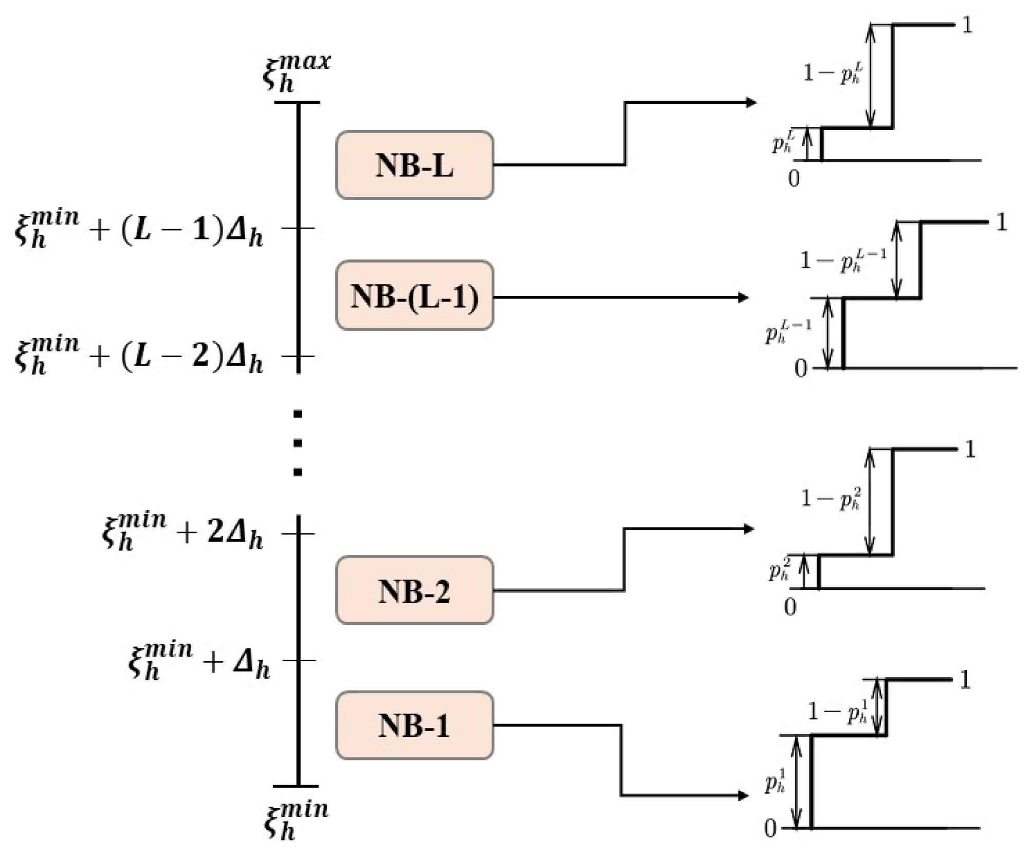
Finally, an NB binary classifier model is trained for each error interval at hour . This approach is chosen because the results of each NB model will serve as evidence for the DST. Training a single multi-class NB classifier would result in only one mass function, where estimated probabilities for each class sum to ‘1’ and individual class probabilities do not form meaningful evidence for the DST. To train the NB classifier for hour h, the day-ahead weather forecast data () and solar power forecast data ( are used as predictors (). The target is represented as a binary class label, , where ‘0’ represents the event that the forecast error falls outside the corresponding interval and ‘1’ represents the event that the forecast error falls inside the corresponding interval. Mathematically, the labeling can be written as follows:
where is the class label of a training sample of the NB classifier of hour and is an indicator function.
NB classifiers are trained using dataset Tr2 and validated through the k-fold cross-validation technique [31]. For the interval at hour , the NB classifier provides two probabilities: one for the forecast falling into the interval () and another for it falling out of the interval (), where . This procedure is illustrated in Figure 2.
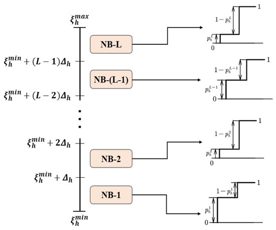
Figure 2.
NB classifiers and corresponding probability outputs for forecast intervals at hour, .
2.3. Probability Estimation with the NB Method
The NB method, a straightforward probabilistic classification algorithm based on Bayes’ theorem of probabilistic inference [32], serves as a crucial tool in this study. Bayes’ theorem connects the conditional and marginal probabilities of two random variables and is often used to calculate posterior probabilities based on given data. In this study, the NB method is used to estimate , i.e., the probability of forecast errors falling into interval given the predictor feature vector .
To be concise, the following study will be focused on interval l at hour h of day d, so that the superscripts l and h can be dropped. Assume that the training data are given for . Here, is the total number of days in Tr2. Symbol is a -dimensional feature vector, which consists of day-ahead weather forecast and solar power forecast . Symbol is the corresponding class label defined in (2). An NB classifier computes the probabilities that an unclassified sample belongs to certain class label(s) conditioned on the feature values using Bayes’ theorem, as depicted in (3).
Here, is the class label, is the probability density function (PDF) of feature vector given that attains class label , and is the prior probability of class . It is assumed that the prior probability follows a Bernoulli distribution.
The NB classifier assumes conditional independence of the features, meaning that the value of a particular feature is considered independent of other features for a given class, as expressed in (4).
Although this assumption may not always hold in some practical applications, NB classifiers, when coupled with kernel density estimation (KDE), can still achieve accurate estimations in such cases [32]. KDE is a non-parametric estimation technique for estimating PDF, which can be described by (5).
Here, represents the KDE of the PDF of a random variable given realizations of , . The smoothing parameter is also known as bandwidth. Additionally, denotes the kernel function. A commonly used choice for this function is the Gaussian kernel, which is defined in (6).
The KDE of the conditional PDF of the feature vector given Y = C can be obtained through (7). Here, is the number of training samples belonging to class and is the bandwidth for the feature for class and selected to optimize the Gaussian kernel in (6).
An NB classifier for a specific error interval is trained by simultaneously simulating (3) and (7) for each training sample of the corresponding interval of a particular hour in dataset Tr2. The output probabilities of an NB classifier for the interval of hour can be written as (8) and (9).
2.4. Review of the DST
The DST is a mathematical framework employed to combine evidence from multiple independent sources in the presence of uncertainty [26,33]. The DST operates by collecting information from individual sources represented by a mass function, also known as (a.k.a.) the basic probability assignment (BPA). The BPAs are then merged using Dempster’s rule of combination to determine the degrees of belief in a set of events of interest.
When formulating a problem for DST application, a set of all possible solutions, a.k.a. the frame of discernment, is considered. It is assumed that the events of interest are subsets of this frame. Let represent frame of discernment and represent an event of interest, where . Then, represents the events in that are distinct from event . The BPA for is a function that has the following two properties:
- (1)
- , where denotes the empty set
- (2)
- where is the degree of belief assigned to event .
Let represent the BPAs for independent evidence in support of event from . Dempster’s rule of combination can be exploited to construct a new mass function for combined evidence in support of using (10).
Here, denotes the operator for Dempster’s rule of combination, which performs orthogonal sum of mass functions supporting event . And is a normalization constant representing the degree of conflict between individual BPAs, as described by (11).
2.5. Incorporating Evidence from NB Classifiers Using the DST
The NB classifiers provide individual probabilities indicating the likelihood of forecast errors falling within a specific interval. To accurately determine the final probability of an error falling into a specified interval, DST is used to combine the evidence that the error falls into that interval with the evidence that error does not fall into any other intervals. Because there are possible intervals for the error at hour , there are possible events, which are denoted as . Here, represents the event that the error falls into interval , where . The frame of discernment at hour , denoted by , can be written as (12).
The mass functions of these individual events, also known as BPAs, are obtained from the NB classifiers. The mass function of the event is defined in (13)–(14) for all values of . Here, denotes the event that the error does not fall into the interval.
Because solar generation is inherently non-negative and cannot exceed the generation capacity of the solar power plant, the constraint described by (15) is imposed on solar power generation. Here, represents the maximum generation capacity of the solar power plant.
The range of the forecast error is then established using (16) and (17). The bounds on the index of error interval are set through (18)–(19). Here, represents the ceiling operation and and are the indices of the lowermost and uppermost error intervals such that .
The frame of discernment is updated according to the lowermost and uppermost error intervals, as shown in (20).
Here, instead of combining the evidence from the whole set of error intervals, the frame of discernment is shrunk to a subset of intervals, where and . Next, integrate these pieces of evidence using (10) and (11) to determine the probabilities of the forecast errors that fall into each of these intervals, which constitute the mass function , as illustrated in (21).
The CDF of the forecast error is derived by accumulating the probabilities. The set of error values and their corresponding probabilities for the CDF is calculated using the interval bounds and the width, as outlined in (22)–(25).
Finally, the CDF of the solar generation at hour is calculated by adding the day-ahead deterministic forecast to the error values for hour , as shown in (26). Here, represents the NB-DST forecast whose CDF value is .
The framework of the NB-DST method is summarized in Figure 3. In this study, the NB-DST method is coupled with three deterministic forecasting methods: SVR, ANN, and QR (median only), resulting in SVR-NB-DST, QR-NB-DST, and ANN-NB-DST models, respectively. To mitigate the risk of overfitting the NB-DST models to the training data, a separate dataset, TS, is reserved for generating performance metrics to evaluate the models’ effectiveness.
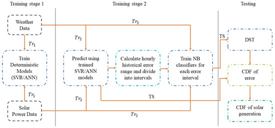
Figure 3.
Framework of the proposed NB-DST method.
3. Performance Metrics for Evaluating Probabilistic Forecasts
Assessing probabilistic forecasts is more challenging than deterministic ones because probabilistic forecasts have various statistical properties. As can be found in the literature, many state-of-the-art probabilistic forecasting methods are only assessed using certain sets of evaluation metrics. But the evaluation process needs to balance several critical aspects, such as forecast accuracy, reliability, sharpness, and uncertainty. This paper aims at addressing this challenge by evaluating the probabilistic forecasting methods using a handful of metrics that assess distinct aspects of the forecasts, providing the forecasters with a framework for critical evaluation. In this section, these evaluation metrics are defined to evaluate the performance of the probabilistic forecasts.
3.1. Continuous Rank Probability Score
The continuous rank probability score (CRPS) is an evaluation metric widely used in various forecasting domains, such as weather, solar and wind power, and load forecasting [5,34,35]. It effectively measures forecast accuracy, reliability, and sharpness. CRPS is defined in (27).
Here, represents the CDF of the forecast at instant . Symbol denotes the CDF of the observation at instance , which is defined as . Here, is an indicator function and denotes the observed value of solar generation. stands for the total number of forecast instances in dataset TS.
A lower CRPS value is desirable as it indicates that the estimated CDF has a lower spread around the observation. It is evident from (27) that the CRPS penalizes any discrepancies between the forecasted CDF and the actual observations. Moreover, for a deterministic forecast, the CRPS transforms into the mean absolute error (MAE). This property makes the CRPS a preferred metric for comparing probabilistic and deterministic forecasts. CRPS can be further decomposed into three components as outlined in (28) [36]. The methods for calculating CRPS, along with its components—REL, UNC, and RES—are detailed in [36] and used in this paper.
3.2. Brier Score
The Brier score (BS) is a scoring function widely used to measure the accuracy of probabilistic forecasts [37]. The BS for a probabilistic forecast at hour is defined in (29).
Here, represents the forecasted probability of event happening at hour h. Term is defined as . denotes the total number of events considered in the probability forecast at hour . To compute the BS for an entire day’s forecast, one can average across all hours, from , where represents the total number of hours of the day.
3.3. Prediction Interval Coverage Probability
After the CDF of the forecast is obtained from a probabilistic forecasting method, a prediction interval (PI) of the forecast can be calculated. For a confidence level of , the PI is determined using (30). Here, represents the quantile of the forecasted CDF, meaning .
The prediction interval coverage probability (PICP) is a measure of the reliability of a probabilistic forecasting method. PICP can be calculated from the PI as outlined in (31) [38].
Here, denotes the forecast at hour , denotes the total number of forecasting hours in a day, and is an indicator function. A forecasting method is considered more reliable if its is closer to the nominal coverage for the confidence intervals of the same size.
3.4. Prediction Interval Normalized Average Width
The prediction interval normalized average width (PINAW) is a metric for measuring the sharpness of a probabilistic forecast method [38]. Mathematically, PINAW is defined in (32), where denotes the observed solar generation at hour on the forecast day. In this formula, the numerator computes the average width of the PI of the probabilistic forecast, while the denominator computes the average hourly solar power generation. A lower PINAW value is desirable, as it indicates a shaper forecast.
3.5. Coverage Width Criterion
The coverage width criterion (CWC) is defined in (33) [39] and can effectively address the limitations of both the PICP and PINAW. While PICP values closer to the nominal coverage indicate a more reliable forecast, they do not assess the sharpness of the forecast. Conversely, a lower PINAW signifies a sharper forecast but does not measure its reliability. The CWC integrates both PICP and PINAW, providing a comprehensive metric to evaluate the reliability and sharpness of a forecast simultaneously.
Here, represents the prediction interval nominal coverage. Symbols and represent hyperparameters, which are chosen as suggested in [39]. A lower CWC value is desirable, as it indicates that a probabilistic forecasting method is more reliable and sharper.
4. Case Study
In this section, day-ahead probabilistic forecasting of solar PV generation is performed using the proposed NB-DST method. In addition to the SVR-NB-DST, QR-NB-DST, and ANN-NB-DST methods, the study also implements the AnEn and PerEn methods [21] as benchmarks. Although there are many probabilistic methods in the literature, they have not been widely adopted in practice. For example, the PerEn method is still preferred for benchmarking within both industry settings and research environments, such as those conducted by the US Department of Energy [40]. The effectiveness of these methods is evaluated and compared using the performance metrics outlined in Section 3 using real-world data.
4.1. Data Collection and Selection
The solar generation data used in this study are collected from a 450-kW solar PV plant located on the rooftop of the Target® store in Vestal, NY, USA (latitude 42°05′37.0″ N, longitude 76°00′06.0″ W). This plant was established in 2016 with support from the New York State Energy Research and Development Authority (NYSERDA). Hourly solar generation data of this plant between 2016 and 2022 are downloaded from NYSERDA’s website [41].
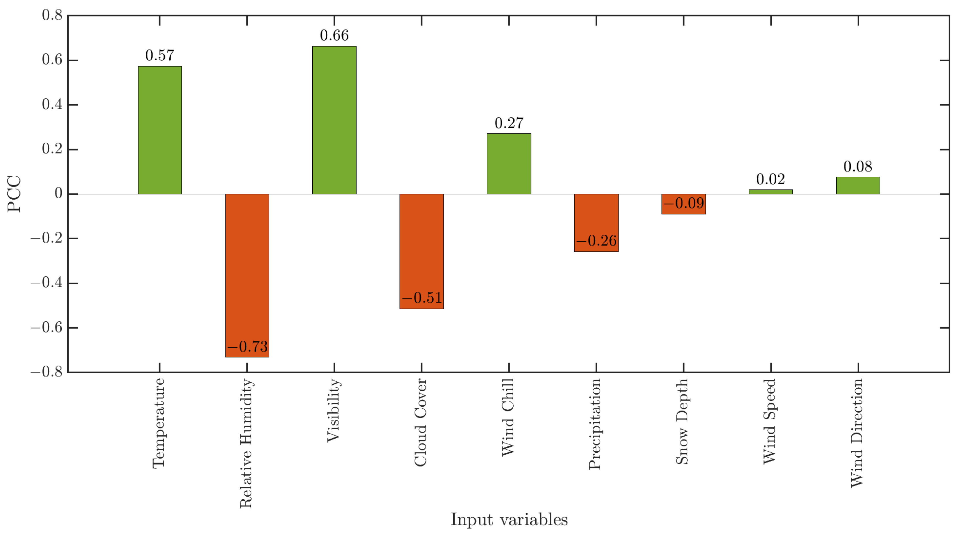
Additionally, this study incorporates various weather variables that significantly influence solar irradiance [42]. Historical weather data for the study site from 2016 to 2021, along with historical forecast data for 2022, are collected on an hourly basis from the website of Visual Crossing weather data service [43]. The weather variables available in this dataset are listed in Table 1. To select the predictor variables for the forecasting algorithms, the correlation between solar generation and each numerical weather variable is measured using Pearson’s correlation coefficient (PCC) [44]. After pre-processing and removing outliers from the data, the PCC for each numerical weather predictor variable with solar generation data is calculated. The results are presented in Figure 4. It is observed that temperature and visibility have a strong positive correlation with solar power generation, while relative humidity and cloud cover have a strong negative correlation. The correlations of other predictor variables are weak, as shown in Figure 4, and thus, these variables are excluded from the model. Solar generation data from the previous day’s corresponding hours are also included in the model to account for the auto-correlation of the solar power generation data.

Table 1.
Weather variables for the study site are available from the Visual Crossing weather data service (2016–2022).

Figure 4.
PCC of weather variables with the hourly solar generation data.
The datasets used in this study are divided as follows: the data from 2016 to 2019 are designated as the Tr1 dataset, while data recorded from 2020 to 2021 are used as the Tr2 dataset. The data recorded in 2022 are used as the TS dataset. Because weather conditions are complex and have varying impacts on solar PV generation, separate forecasting models are built and evaluated under different cloud patterns. Accordingly, the datasets are further divided into three categories on a daily basis according to the weather conditions using the approach described in [45]: “clear”, “overcast”, and “partially cloudy”. The daily solar generation profile on a clear day typically exhibits a smooth bell curve, with the power generation peaking near the generation capacity during noon. On overcast days, the total daily solar generation is significantly lower. On partially cloudy days, the hourly solar generation shows considerable fluctuation, characterized by multiple peaks and troughs throughout the day.
Subsequently, the forecasting models are first trained using Tr1 and Tr2 datasets for each hour of the day under these distinct weather conditions. Then, the forecasting models are evaluated using the performance metrics computed through the TS dataset. Note that out of 365 days in the TS dataset, there are 124 days classified as “clear”, 129 days classified as “overcast”, and 112 days classified as “partially cloudy”. The effectiveness of the forecasting models is evaluated using a -fold cross-validation approach.
4.2. Performance Evaluation under “Clear” Weather Conditions
This subsection focuses on assessing the probabilistic forecasting methods during “clear” weather conditions. The performance metrics for the 124 “clear” days in the TS dataset are calculated for all the methods and summarized in Table 2. It can be observed from Table 2 that the three NB-DST methods outperform the AnEn and PerEn methods in terms of the CRPS. Also, the BS values for the NB-DST methods are considerably lower than those for the other methods, which indicates NB-DST’s higher accuracy. These three NB-DST methods show satisfactory reliability and coverage with resolution metrics notably surpassing those of the AnEn and PerEn methods. Also, a slightly lower value of the PINAW for the ANN-NB-DST gives it an advantage over the other two NB-DST methods. While the PICP values for the three NB-DST methods are comparable to those for the AnEn and PerEn methods, the NB-DST methods, particularly ANN-NB-DST, exhibit superior overall performance as indicated by their lower CWC values.

Table 2.
Performance metrics of all the forecasting methods evaluated over the 124 “Clear” days.
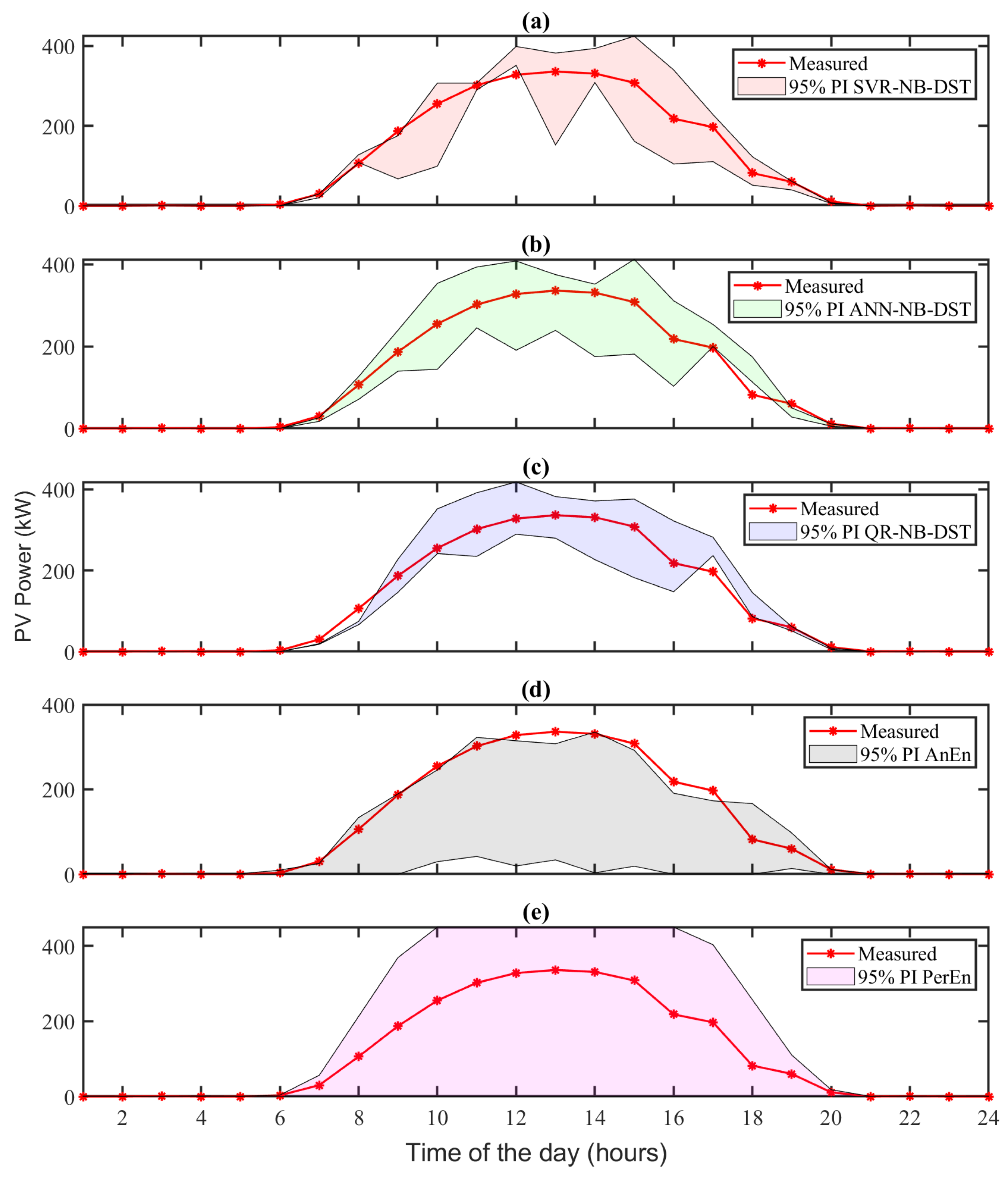
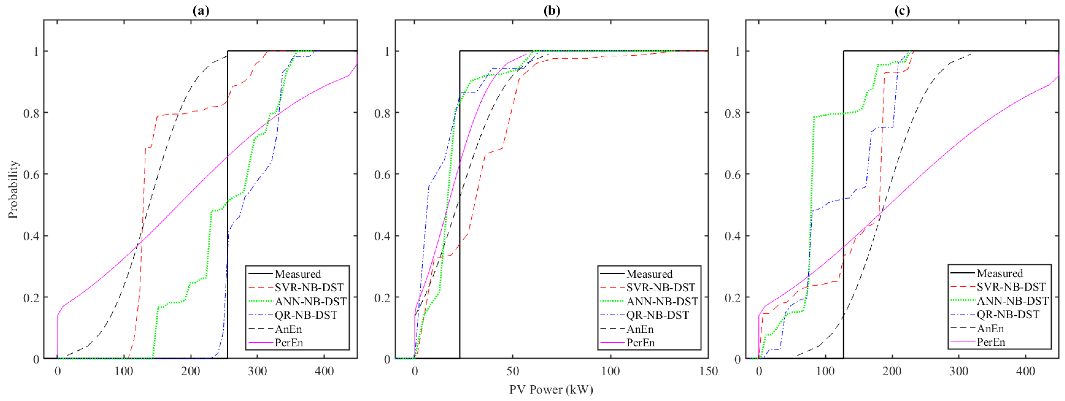
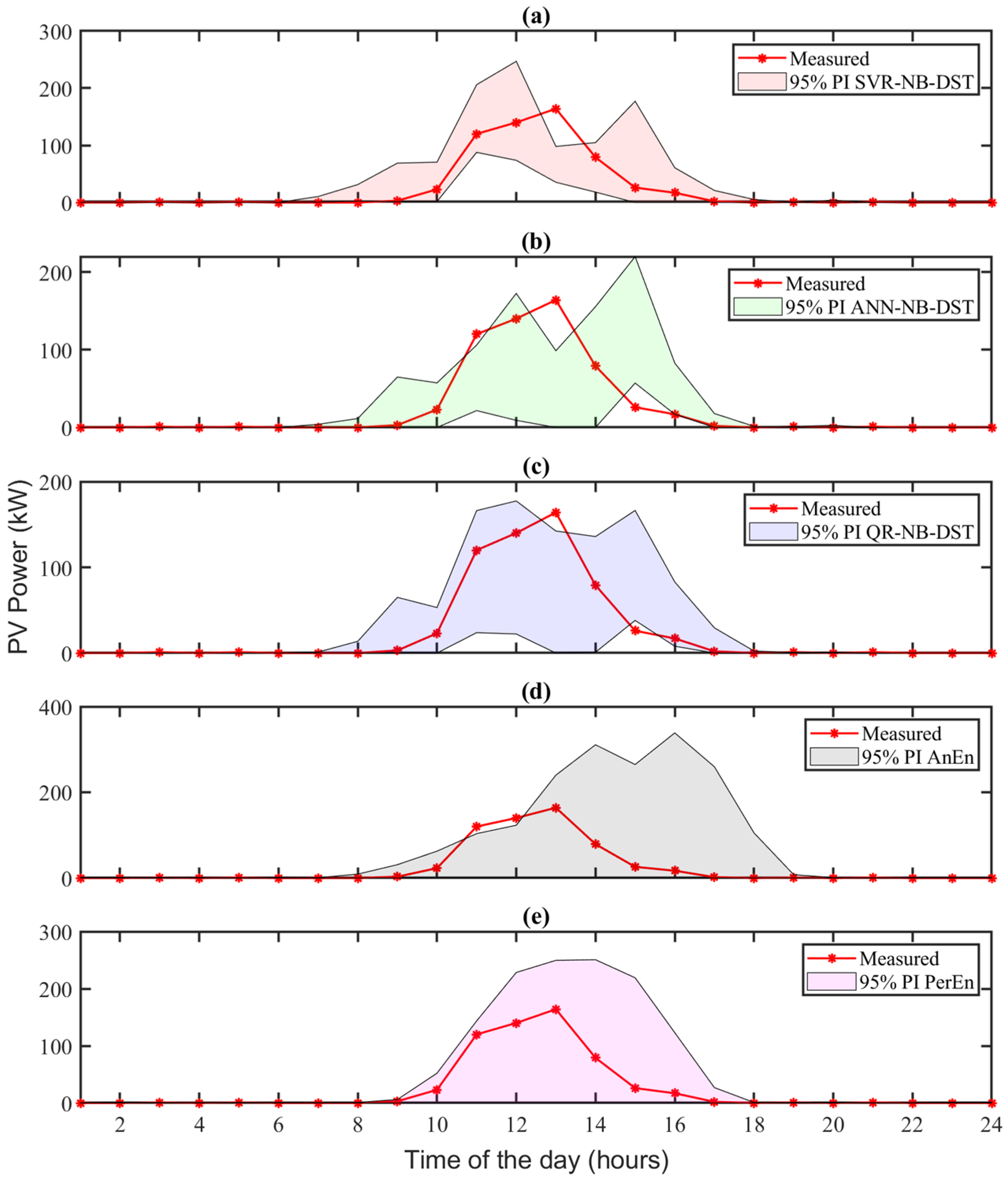
To further illustrate the performance, Figure 5 shows the estimated 95% PIs from all the forecasting methods for a particular “clear” day (19 May 2022). The 95% PIs are obtained using (22) by setting α = 0.05. It can be observed that the 95% PIs of the three NB-DST methods are narrower than those of the two benchmark methods. Figure 6a shows the CDF estimate for PV power at 10:00 AM on this “clear” day (19 May 2022). It can be observed that the CDFs estimated using the ANN-NB-DST and the QR-NB-DST methods exhibit the lowest deviation from the actual observation CDF. Although the CDF estimated by the SVR-NB-DST method shows a deviation slightly higher than other NB-DST methods, it still performs commendably when compared to the benchmark methods.
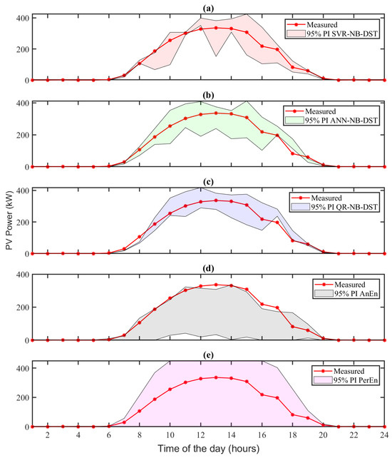
Figure 5.
The 95% PIs obtained from all the probabilistic solar forecasting methods on a particular “clear” day (19 May 2022), with regard to (a) SVR-NB-DST, (b) ANN-NB-DST, (c) QR-NB-DST, (d) AnEn, and (e) PerEn. The red dotted lines denote the actual hourly observations of solar power and the shaded areas denote the 95% PIs of the forecasted solar generation obtained from the corresponding methods.
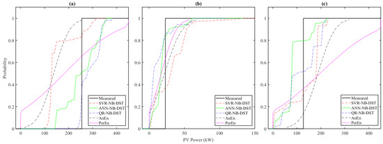
Figure 6.
Estimated CDFs of the PV power using all the probabilistic forecasting methods at 10:00 AM on (a) a “clear” day (19 May 2022), (b) an “overcast” day (18 December 2022), and (c) a “partially cloudy” day (9 July 2022). The solid black line represents the CDF of the actual observation.
4.3. Performance Evaluation under “Overcast” Weather Conditions
In this subsection, the performance metrics are calculated over the 129 “overcast” days in the TS dataset for all the probabilistic forecasting methods and are summarized in Table 3. Among these methods, the ANN-NB-DST stands out by achieving the lowest CRPS. It also exhibits superior reliability and resolution, as indicated by its REL and RES values, compared to the other methods. Notably, the resolution of all the NB-DST methods is superior to the two benchmark methods as their PINAW values are much lower. While the PICP values for the NB-DST methods are further from the ideal 95% nominal coverage than the benchmark methods, their lower CWC values reflect better overall performance considering both forecast reliability and sharpness. Additionally, the lower BS values of the NB-DST methods suggest that the NB-DST methods are more accurate than the other methods. Among the three NB-DST methods, the ANN-NB-DST method exhibits the most impressive performance.

Table 3.
Performance metrics of all the forecasting methods evaluated over the 129 “Overcast” days.
To further illustrate the performance, Figure 7 shows the 95% PIs obtained from the forecasting methods on a particular “overcast” day (28 December 2022). It can be observed that the 95% PIs for the AnEn and PerEn methods are notably broader than those for the NB-DST methods. Additionally, the SVR-NB-DST method meets the targeted coverage rate of 95% PIs, whereas the coverage rates of the ANN-NB-DST and QR-NB-DST methods are lower than the targeted 95%. This variation highlights the challenges of forecasting under overcast conditions. The estimated CDFs of the hourly solar generation estimated by the forecasting methods at 10:00 AM on this “overcast” day (28 December 2022) are illustrated in Figure 6b. It can be observed from Figure 6b that the CDFs estimated by the NB-DST methods align more closely to the actual observation CDF than those estimated by the two benchmark methods.
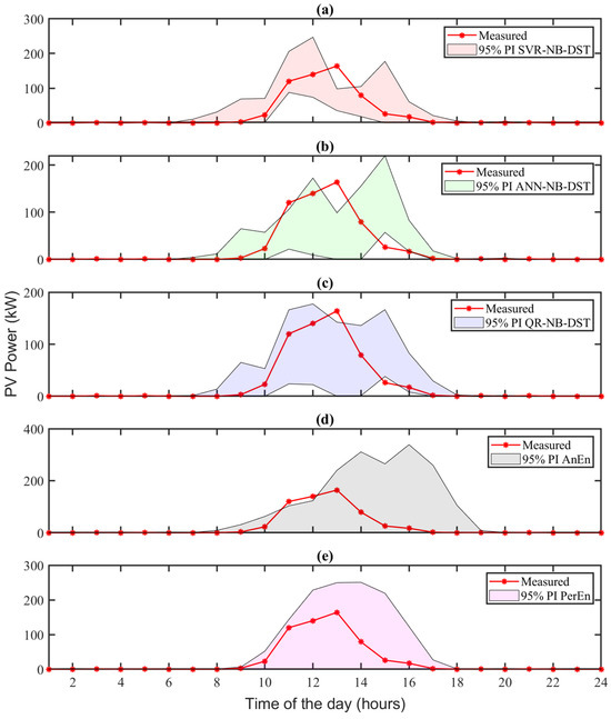
Figure 7.
The 95% PIs obtained from all the probabilistic solar forecasting methods on a particular “overcast” day (28 December 2022): (a) SVR-NB-DST, (b) ANN-NB-DST, (c) QR-NB-DST, and (d) AnEn, and (e) PerEn.
4.4. Performance Evaluation under “Partially Cloudy” Weather Conditions
In this subsection, the performance metrics are calculated over the 112 “partially cloudy” days in the TS dataset for all the probabilistic forecasting methods and are summarized in Table 4. It can be observed that the ANN-NB-DST method achieves the lowest CRPS value, which indicates the best overall performance. Additionally, the reliability and resolution of the ANN-NB-DST method are also superior to those of other NB-DST and benchmark methods, as indicated by its lower value of REL and higher value of RES. Moreover, the lower PINAW values of the NB-DST methods suggest that they have better resolution than the AnEn and the PerEn methods. While the PICP values for the NB-DST methods are not as good as those for the benchmark methods, the CWC values, which consider both PICP and PINAW, suggest a better overall performance for the NB-DST methods. Notably, the ANN-NB-DST method stands out with the lowest BS, indicating the highest accuracy among the five methods.

Table 4.
Performance metrics of all the forecasting methods were evaluated over the 112 “partially cloudy” days.
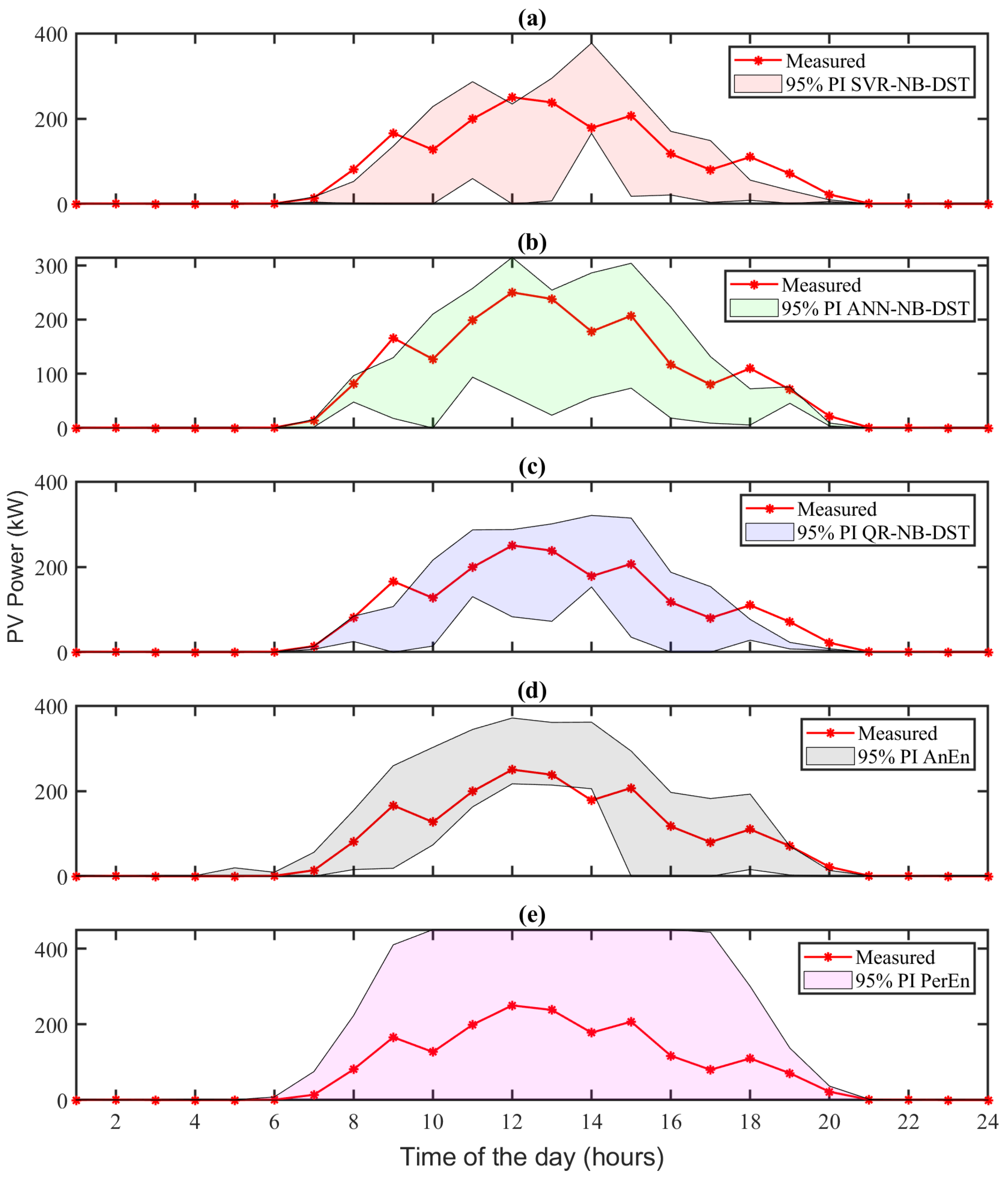
To further illustrate the performance, Figure 8 shows the 95% PIs obtained from all the forecasting methods on a particular “partially cloudy” day (9 July 2022). It can be observed that the 95% PIs obtained from the benchmark methods are wider than those from the NB-DST methods. Also, in Figure 8, some measured points fall outside the 95% PIs obtained from the CDFs estimated by the NB-DST methods. In contrast, such occurrences are not observed with the AnEn and PerEn methods. The observation highlights a strategic trade-off made by the NB-DST methods, prioritizing improved resolution over coverage probability. Figure 6c shows the CDFs estimated by all the methods at 10:00 AM on this “partially cloudy” day (9 July 2022). The CDFs estimated by the NB-DST methods show smaller deviations from the actual observed solar power CDF than those estimated by the AnEn and PerEn methods.
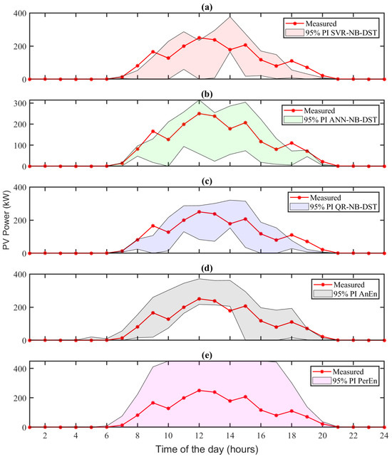
Figure 8.
The 95% PIs obtained from all the probabilistic solar forecasting methods on a particular “partially cloudy” day (9 July 2022): (a) SVR-NB-DST, (b) ANN-NB-DST, (c) QR-NB-DST, (d) AnEn, and (e) PerEn.
4.5. Overall Comparative Analysis
The results from Table 2, Table 3 and Table 4 are synthesized to evaluate the overall performance of the proposed method over the 1-year testing dataset, TS. The findings are presented in Table 5. Notably, the NB-DST methods outperform the benchmark methods on nearly all performance metrics except for the PICP. This exception is understandable because the PI estimates of the PerEn and AnEn methods are considerably wider than those of the NB-DST methods. Even with the exception, the significantly better PINAW and CWC values suggest the overall superiority of the NB-DST methods. According to Table 5, the ANN-NB-DST emerges as the best-performing method among the NB-DST variants.

Table 5.
Performance metrics of all the forecasting methods evaluated over the 1-year testing dataset.
Figure 9 further illustrates the percentage improvements in CRPS and CWC of the ANN-NB-DST method over the PerEn method across all weather conditions. As explained before, CRPS measures the overall deviation of the estimated CDF from the actual measurements, indicating the forecast accuracy, while CWC measures the reliability and sharpness of the forecasted CDF. Notably, the ANN-NB-DST method achieves over 33% improvement in CRPS under clear and partially cloudy weather conditions. This result indicates that the CDF estimated by the ANN-NB-DST method deviates less from the actual solar power measurements than the PerEn method. Also, the improvement in CRPS is less pronounced (<10%) under overcast weather conditions, reflecting the challenges in predictive accuracy under such weather. Despite this, results from Figure 7 and Table 3 suggest the overall superiority of the ANN-NB-DST method in accuracy and sharpness with a slight reduction in reliability. Moreover, the CWC improvement remains consistent (more than 52%) across all the weather conditions, indicating the higher reliability and better sharpness of the ANN-NB-DST method than the benchmark method.
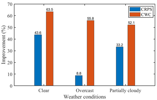
Figure 9.
Comparative improvement in the ANN-NB-DST method over the widely used benchmark, the PerEn method.
5. Conclusions and Future Work
This paper proposes the NB-DST method, a novel approach for quantifying forecast errors of a deterministic forecasting method by estimating the CDF using a non-parametric technique. The NB-DST method has been integrated with deterministic forecasting methods such as SVR, ANN, and QR to generate probabilistic forecasts under different weather conditions. Comparisons with established benchmark methods (AnEn and PerEn) using real-world data reveal that the NB-DST methods consistently outperform the benchmarks in terms of lower CRPS, BS, and CWC values. Among the tested methods, the ANN-NB-DST method emerges as the top performer, consistently producing reliable and high-resolution CDF estimates across various weather conditions, establishing it as the superior option for probabilistic photovoltaic (PV) forecasting among the methods evaluated.
Future studies will focus on exploring a wider range of deterministic forecasting methods in conjunction with the NB-DST method to enhance forecast robustness and consistency. Additionally, this study considered only a limited number of meteorological variables due to data availability limitations. Thus, an important direction for future investigation is to incorporate a more comprehensive set of meteorological variables into the forecasting models. This expansion will enable a deeper exploration of their impact on forecasting accuracy and provide more comprehensive insights into the dynamics of probabilistic PV forecasting.
Author Contributions
T.A.: Methodology, Data curation, Software, Visualization, Investigation, Validation, and Writing—original draft. N.Z.: Conceptualization, Supervision, and Writing—review and editing. Z.Z.: Writing—review and editing. W.T.: Writing—review and editing. All authors have read and agreed to the published version of the manuscript.
Funding
This paper is based on work supported by the U.S. National Science Foundation under grant #1845523 and by the U.S. Department of Energy’s Office of Energy Efficiency and Renewable Energy (EERE) under the Solar Energy Technologies Office Award Number DE-EE0009341. The views, findings, conclusions, and recommendations presented in this paper are solely those of the authors and do not necessarily reflect those of the funding agencies.
Data Availability Statement
The historical solar power generation data used in this study can be found at https://der.nyserda.ny.gov/reports/view/performance/?project=318 (accessed on 31 March 2024), and the related weather data can be downloaded from https://www.visualcrossing.com/weather/weather-data-services#/editDataDefinition (accessed on 31 March 2024) [41,43].
Conflicts of Interest
The authors declare that they have no known competing financial interests or personal relationships that could have appeared to influence the work reported in this paper.
References
- Li, B.; Zhang, J. A review on the integration of probabilistic solar forecasting in power systems. Sol. Energy 2020, 210, 68–86. [Google Scholar] [CrossRef]
- González, J.M.M.; Conejo, A.J.; Madsen, H.; Pinson, P.; Zugno, M. Integrating Renewables in Electricity Markets: Operational Problems; Springer: New York, NY, USA, 2014; Volume 205, p. 429. [Google Scholar]
- Kaur, A.; Nonnenmacher, L.; Pedro, H.T.; Coimbra, C.F. Benefits of solar forecasting for energy imbalance markets. Renew. Energy 2016, 86, 819–830. [Google Scholar] [CrossRef]
- Notton, G.; Nivet, M.-L.; Voyant, C.; Paoli, C.; Darras, C.; Motte, F.; Fouilloy, A. Intermittent and stochastic character of renewable energy sources: Consequences, cost of intermittence and benefit of forecasting. Renew. Sustain. Energy Rev. 2018, 87, 96–105. [Google Scholar] [CrossRef]
- Gneiting, T.; Katzfuss, M. Probabilistic forecasting. Annu. Rev. Stat. Appl. 2014, 1, 125–151. [Google Scholar] [CrossRef]
- Abdel-Nasser, M.; Mahmoud, K. Accurate photovoltaic power forecasting models using deep LSTM-RNN. Neural Comput. Appl. 2019, 31, 2727–2740. [Google Scholar] [CrossRef]
- Aprillia, H.; Yang, H.-T.; Huang, C.-M. Short-term photovoltaic power forecasting using a convolutional neural network–salp swarm algorithm. Energies 2020, 13, 1879. [Google Scholar] [CrossRef]
- Michael, E.; Neethu, M.M.; Hasan, S.; Al-Durra, A. Short-term solar power predicting model based on multi-step CNN stacked LSTM technique. Energies 2022, 15, 2150. [Google Scholar] [CrossRef]
- Huang, X.; Li, Q.; Tai, Y.; Chen, Z.; Zhang, J.; Shi, J.; Gao, B.; Liu, W. Hybrid deep neural model for hourly solar irradiance forecasting. Renew. Energy 2021, 171, 1041–1060. [Google Scholar] [CrossRef]
- Zang, H.; Liu, L.; Sun, L.; Cheng, L.; Wei, Z.; Sun, G. Short-term global horizontal irradiance forecasting based on a hybrid CNN-LSTM model with spatiotemporal correlations. Renew. Energy 2020, 160, 26–41. [Google Scholar] [CrossRef]
- Pazikadin, A.R.; Rifai, D.; Ali, K.; Malik, M.Z.; Abdalla, A.N.; Faraj, M.A. Solar irradiance measurement instrumentation and power solar generation forecasting based on Artificial Neural Networks (ANN): A review of five years research trend. Sci. Total Environ. 2020, 715, 136848. [Google Scholar] [CrossRef]
- Yadav, A.P.; Kumar, A.; Behera, L. RNN based solar radiation forecasting using adaptive learning rate. In Proceedings of the Swarm, Evolutionary, and Memetic Computing: 4th International Conference, SEMCCO 2013, Chennai, India, 19–21 December 2013. [Google Scholar]
- Liu, C.-H.; Gu, J.-C.; Yang, M.-T. A simplified LSTM neural networks for one day-ahead solar power forecasting. IEEE Access 2021, 9, 17174–17195. [Google Scholar] [CrossRef]
- Feng, C.; Liu, Y.; Zhang, J. A taxonomical review on recent artificial intelligence applications to PV integration into power grids. Int. J. Electr. Power Energy Syst. 2021, 132, 107176. [Google Scholar] [CrossRef]
- Abuella, M.; Chowdhury, B. Solar power forecasting using support vector regression. In Proceedings of the International Annual Conference of the American Society for Engineering Management, Charlotte, NC, USA, 26–29 October 2016. [Google Scholar]
- Fentis, A.; Bahatti, L.; Mestari, M.; Tabaa, M.; Jarrou, A.; Chouri, B. Short-term PV power forecasting using support vector regression and local monitoring data. In Proceedings of the 2016 International Renewable and Sustainable Energy Conference (IRSEC), Marrakech, Morocco, 14–17 November 2016. [Google Scholar]
- Abuella, M.; Chowdhury, B. Hourly probabilistic forecasting of solar power. In Proceedings of the 2017 North American Power Symposium (NAPS), Morgantown, WV, USA, 17–19 September 2017. [Google Scholar]
- Mohammed, A.A.; Aung, Z. Ensemble learning approach for probabilistic forecasting of solar power generation. Energies 2016, 9, 1017. [Google Scholar] [CrossRef]
- Zhang, Y.-M.; Wang, H. Multi-head attention-based probabilistic CNN-BiLSTM for day-ahead wind speed forecasting. Energy 2023, 278, 127865. [Google Scholar] [CrossRef]
- Lauret, P.; David, M.; Pedro, H.T.C. Probabilistic solar forecasting using quantile regression models. Energies 2017, 10, 1591. [Google Scholar] [CrossRef]
- Alessandrini, S.; Monache, L.D.; Sperati, S.; Cervone, G. An analog ensemble for short-term probabilistic solar power forecast. Appl. Energy 2015, 157, 95–110. [Google Scholar] [CrossRef]
- Doubleday, K.; Jascourt, S.; Kleiber, W.; Hodge, B.-M. Probabilistic solar power forecasting using bayesian model averaging. IEEE Trans. Sustain. Energy 2020, 12, 325–337. [Google Scholar] [CrossRef]
- Najibi, F.; Apostolopoulou, D.; Alonso, E. Enhanced performance Gaussian process regression for probabilistic short-term solar output forecast. Int. J. Electr. Power Energy Syst. 2021, 130, 106916. [Google Scholar] [CrossRef]
- Wang, H.; Zhang, Y.-M.; Mao, J.-X. Sparse Gaussian process regression for multi-step ahead forecasting of wind gusts combining numerical weather predictions and on-site measurements. J. Wind. Eng. Ind. Aerodyn. 2022, 220, 104873. [Google Scholar] [CrossRef]
- Dahl, A.; Bonilla, E. Scalable Gaussian process models for solar power forecasting. In Proceedings of the Data Analytics for Renewable Energy Integration: Informing the Generation and Distribution of Renewable Energy: 5th ECML PKDD Workshop, DARE, Skopje, Macedonia, 22 September 2017. [Google Scholar]
- Wilson, N. Algorithms for dempster-shafer theory. In Handbook of Defeasible Reasoning and Uncertainty Management Systems: Algorithms for Uncertainty and Defeasible Reasoning; Springer: Dordrecht, The Netherlands, 2000; pp. 421–475. [Google Scholar]
- Wang, H.; Zhang, Y.-M.; Mao, J.-X.; Wan, H.-P. A probabilistic approach for short-term prediction of wind gust speed using ensemble learning. J. Wind Eng. Ind. Aerodyn. 2020, 202, 104198. [Google Scholar] [CrossRef]
- Yang, M.; Lin, Y.; Han, X. Probabilistic wind generation forecast based on sparse Bayesian classification and Dempster–Shafer theory. IEEE Trans. Ind. Appl. 2016, 52, 1998–2005. [Google Scholar] [CrossRef]
- Ng, A.; Jordan, M. On discriminative vs. generative classifiers: A comparison of logistic regression and naive bayes. Adv. Neural Inf. Process. Syst. 2001, 14, 841–848. [Google Scholar]
- Blázquez-García, A.; Conde, A.; Mori, U.; Lozano, J.A. A review on outlier/anomaly detection in time series data. ACM Comput. Surv. (CSUR) 2021, 54, 1–33. [Google Scholar] [CrossRef]
- Fushiki, T. Estimation of prediction error by using K-fold cross-validation. Stat. Comput. 2011, 21, 137–146. [Google Scholar] [CrossRef]
- Hastie, T.; Tibshirani, R.; Friedman, J.H.; Friedman, J.H. The Elements of Statistical Learning: Data Mining, Inference, and Prediction; Springer: New York, NY, USA, 2009; Volume 2. [Google Scholar]
- Kaltsounidis, A.; Karali, I. Dempster-Shafer Theory: How Constraint Programming Can Help. In Proceedings of the Information Processing and Management of Uncertainty in Knowledge-Based Systems: 18th International Conference, IPMU 2020, Lisbon, Portugal, 15–19 June 2020. [Google Scholar]
- van der Meer, D.; Munkhammar, J.; Widén, J. Probabilistic forecasting of solar power, electricity consumption and net load: Investigating the effect of seasons, aggregation and penetration on prediction intervals. Sol. Energy 2018, 171, 397–413. [Google Scholar] [CrossRef]
- Juban, J.; Siebert, N.; Kariniotakis, G.N. Probabilistic short-term wind power forecasting for the optimal management of wind generation. In Proceedings of the 2007 IEEE Lausanne Power Tech, Lausanne, Switzerland, 1–5 July 2007. [Google Scholar]
- Hersbach, H. Decomposition of the continuous ranked probability score for ensemble prediction systems. Weather Forecast. 2000, 15, 559–570. [Google Scholar] [CrossRef]
- Ferro, C.A. Comparing probabilistic forecasting systems with the Brier score. Weather Forecast. 2007, 22, 1076–1088. [Google Scholar] [CrossRef]
- Lauret, P.; David, M.; Pinson, P. Verification of solar irradiance probabilistic forecasts. Sol. Energy 2019, 194, 254–271. [Google Scholar] [CrossRef]
- Li, C.; Tang, G.; Xue, X.; Chen, X.; Wang, R.; Zhang, C. The short-term interval prediction of wind power using the deep learning model with gradient descend optimization. Renew. Energy 2020, 155, 197–211. [Google Scholar] [CrossRef]
- Solar Energy Technologies Office (SETO). American-Made Solar Forecasting Prize. 2021. Available online: https://www.energy.gov/eere/solar/american-made-solar-forecasting-prize (accessed on 31 March 2024).
- NYSERDA DER Integrated Data System. [Online]. Available online: https://der.nyserda.ny.gov/reports/view/performance/?project=318 (accessed on 26 August 2023).
- Inman, R.H.; Pedro, H.T.; Coimbra, C.F. Solar forecasting methods for renewable energy integration. Prog. Energy Combust. Sci. 2013, 39, 535–576. [Google Scholar] [CrossRef]
- Weather Data Services|Visual Crossing. [Online]. Available online: https://www.visualcrossing.com/weather/weather-data-services#/editDataDefinition (accessed on 26 August 2023).
- Hsing, T.; Liu, L.-Y.; Brun, M.; Dougherty, E.R. The coefficient of intrinsic dependence (feature selection using el CID). Pattern Recognit. 2005, 38, 623–636. [Google Scholar] [CrossRef]
- Liu, Z.; Zhang, Z. Solar forecasting by K-Nearest Neighbors method with weather classification and physical model. In Proceedings of the 2016 North American Power Symposium (NAPS), Denver, CO, USA, 18–20 September 2016. [Google Scholar]
Disclaimer/Publisher’s Note: The statements, opinions and data contained in all publications are solely those of the individual author(s) and contributor(s) and not of MDPI and/or the editor(s). MDPI and/or the editor(s) disclaim responsibility for any injury to people or property resulting from any ideas, methods, instructions or products referred to in the content. |
© 2024 by the authors. Licensee MDPI, Basel, Switzerland. This article is an open access article distributed under the terms and conditions of the Creative Commons Attribution (CC BY) license (https://creativecommons.org/licenses/by/4.0/).


