Application of Neural Network Feedforward in Fuzzy PI Controller for Electric Vehicle Thermal Management System: Modeling and Simulation Studies

Abstract

The electric vehicle thermal management system (EVTMS) plays a crucial role in ensuring battery efficiency, driving range, and passenger comfort. However, EVTMSs still face unresolved challenges, such as accurate modeling, compensating for temperature variations, and achieving efficient control strategies. Addressing these issues is crucial for enhancing the performance, reliability, and energy efficiency of electric vehicles. Therefore, this study presents a cooling EVTMS model, considering both the battery pack temperature and the cabin comfort, and utilizes the prediction of neural network as a feedforward in a fuzzy PI controller to compensate for the model temperature variations. The simulation results reveal that, compared with PI controller and MPC, the neural network fuzzy PI (NN-Fuzzy PI) controller can well predict and compensate for the system’s nonlinear characteristics as well as the time-delay caused by heat transfer, achieving superior control performance and reducing energy consumption. The battery pack temperature and $\mathrm{PMV}$ fluctuations are effectively constrained within [−0.5, 0.5] and [−0.1, 0.1], reducing up to 150% and 164%, and the energy consumption of the pump and compressor are reduced by up to 0.23 and 100.1 $\mathrm{KJ}$, with ranges of 18% and 2.68%. Meanwhile, the neural network feedforward also works effectively in different controllers. The findings of this research can provide valuable insights for TMS engineers to select advanced control strategies.

1. Introduction

Lithium-ion batteries are considered the primary power source for electric vehicles (EVs) due to advantages such as long cycle life, low self-discharge rate, and environmental friendliness [1,2,3,4]. To save space, battery packs are often tightly arranged, leading to heat accumulation during charging and discharging, resulting in temperature rise. Meanwhile, the battery pack characteristics are greatly affected by temperature, as excessive temperature will cause decomposition of internal materials, leading to reduced battery life and even hazardous situations, such as spontaneous combustion. Considering factors such as safety, lifespan, and energy efficiency, it is necessary to limit the battery temperature to 15–35 °C [5,6,7]. Therefore, an effective thermal management system (TMS) is crucial for regulating battery temperature while extending the driving range and ensuring cabin comfort.

So far, many scholars have correlated more subsystems in EVs to form an integrated TMS to control overall variables in the system, which are more representative and can achieve better control performance. References [8,9,10,11,12,13] developed integrated EVTMSs that could not only effectively predict system parameters but also match the most efficient operating modes under different conditions to save energy. Sanket Shah et al. [14] integrated a battery electrochemical model into a battery TMS to predict the battery pack’s cycling and aging. References [15,16,17] developed a TMS for plug-in hybrid electric vehicles (PHEVs) based on environmental and target temperature, which ensured system performance and achieved energy savings. Wang et al. [18] proposed a new control structure for an EVTMS based on refrigerants, aiming to reduce the uneven distribution of refrigerants in the battery cooling plate channels during the heating process.

In the research on TMS control strategies, the finite state machine (FSM) is widely used, which regulates valve switches, fan speeds, and compressor speeds by defining several typical scenarios. Although the FSM is simple, it cannot cover all operating conditions, thereby failing to meet the requirements of high energy efficiency and cabin comfort.

Many scholars have utilized Proportional-Integral-Derivative (PID) control and Fuzzy Control (FC) to seek more efficient control strategies and optimal outcomes. Cen et al. [19] implemented a PID controller to adjust the expansion valve and thermostat of the cooling system to maintain the battery temperature difference within 2 °C. References [20,21] designed TMS control strategies based on Dynamic Programming (DP), which showed that DP controllers were capable of tracking reference temperatures with less power consumption compared with PID controllers; however, due to the lack of feedback, DP controllers also had lower robustness and required more computational time. References [22,23] implemented FC strategies to reduce temperature fluctuations, lifespan degradation, and energy consumption of EV batteries. Sefkat et al. [24] utilized FC strategies to regulate fuel cell temperatures, resulting in energy savings ranging from 15% to 58.74%.

Currently, the application of PID and FC in the TMS is extensively explored. However, due to their rule-based nature that often relies on empirical knowledge, they may not achieve satisfactory control performance when faced with limited empirical data. Therefore, more advanced control strategies are proposed. Wang et al. [25] proposed a hysteresis control method for the TMS, which effectively reduced battery temperature rise and inconsistencies; however, frequent switching in this method might lead to potential damage to devices. Bauer et al. [26] utilized Pontryagin’s maximum principle to determine the optimal battery temperature, considering the trade-off between maximum expected lifespan and minimal energy consumption. Zhang et al. [27] optimized a multistage charging control strategy by using genetic algorithms, which reduced energy consumption by 11.61% and improved charging efficiency by 1.2%. Xie et al. [28] introduced a self-learning intelligent control strategy that improved passenger comfort and reduced energy consumption.

Model Predictive Control (MPC) has also gradually been applied in the TMS due to its superior dynamic control performance and high system robustness. References [29,30] utilized MPC to regulate battery temperature, which proved that the allocation theory effectively enhanced the TMS performance. Tao et al. [31,32] designed a compressor MPC controller which exhibited the excellent performance of MPC in temperature tracking and energy consumption reduction.

Lopez-Sanz et al. [33,34] implemented Nonlinear Model Predictive Control (NMPC) for a TMS, which enabled rapid battery preheating and resulted in a 30% cost reduction. Hua et al. [35] utilized Particle Swarm Optimization (PSO) algorithms to design a nonlinear TMS strategy, which outperformed PID controllers in terms of reducing battery temperature deviations and inconsistencies. References [36,37] used neural networks to control the TMS, which successfully reduced battery temperature inconsistencies, improved energy efficiency, and demonstrated the effectiveness of neural networks for the control of nonlinear and time-varying TMS.

Current research indicates that compared with FSM, control strategies such as PID, FC, and MPC can achieve better control and energy-saving effects in the TMS. However, the complex, nonlinear, time-varying TMS and time delay caused by heat transfer make it challenging to establish an efficient control model. For instance, during the cooling process, the battery temperature may continue to fluctuate even after reaching the target value due to the inherent time delay caused by heat transfer, and it is difficult and unpractical to build an accurate mathematical model of this time delay because of the complexity of TMS. Traditional control methods struggle to effectively respond to such characteristics, resulting in increased energy consumption and more unstable operating conditions. However, there is currently no effective way to solve this problem, which is the focus of this work. We hope to design a new and efficient controller whose structure is different from those widely used at present. In the face of complex nonlinear systems such as EVTMS, it can not only effectively compensate for the time delay caused by heat transfer but also has sufficient robustness to resist unmeasured external interference, thus reducing the control overshoot, further reducing energy consumption and improving driving range.

Based on the above motivations, this study utilizes the strong nonlinear mapping and adaptive capability of backpropagation (BP) neural networks to predict future temperature variations in the EVTMS. The prediction is then used as a feedforward in a Fuzzy-PI control loop to form a neural network fuzzy PI (NN-Fuzzy PI) controller, aiming to reduce control fluctuations. Finally, the EVTMS combined with PI, MPC and NN-Fuzzy PI controllers is simulated under the WLTC condition to evaluate the control performance. The results demonstrate the reduced temperature fluctuations and energy consumption by the NN-Fuzzy PI controller, and meanwhile, the neural network feedforward also performs well in different controllers, which can provide a useful guideline of controller design for EVTMS engineers so as to reduce emissions, save energy and protect the environment.

Meanwhile, in order to obtain effective conclusions, the EVTMS in this paper is integrated with multiple subsystems and thermal comfort models instead of only one single system, which can simultaneously control cabin comfort and battery temperature under summer conditions. The model structure and parameters, as well as the black-box model calibration process of EVTMS, can be used as a reference for engineers and scholars.

The content of this paper is as follows: Section 2: TMS physical model; Section 3: TMS controller; Section 4: simulation results and analysis; Section 5: conclusions.

2. Physical Model

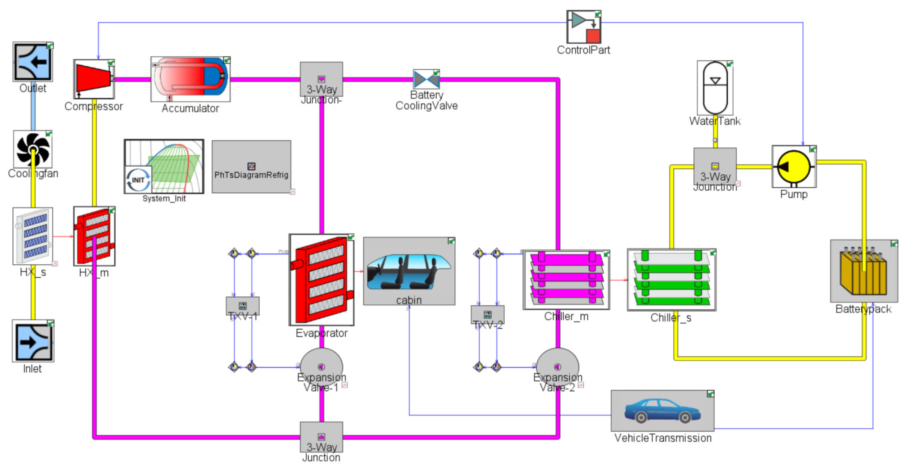
The proposed EVTMS in this study, including a battery cooling circuit and an air-conditioning (AC) circuit, is illustrated in Figure 1. It mainly consists of a compressor, expansion valve, condenser, chiller, battery pack, cabin model, pump, water tank, accumulator, fan, and battery cooling valve. The whole TMS is built based on the commercial software GT-Suite, and the specific parameters of each component are obtained by investigation or the reference value in GT-Suite Library, which is further obtained through test bench and thus can represent the components in real world effectively. Some information about the key components is given below.

2.1. Cabin AC Circuit Model

2.1.1. Compressor Model

The compressor refrigerant mass flow rate $q_m$, enthalpy change $h_{inc}$ and power consumption $P_{comp}$ are calculated according to Equations (1)–(3):

$$q_m=\rho n{\eta }_V{V}_{comp}$$

(1)

$$h_{inc}=\Delta h·{\eta }_{ise}$$

(2)

$$P_{comp}=q_m{h}_{inc}$$

(3)

where $V_{comp}$ represents the compressor displacement;$\rho$ represents the refrigerant density; ${\eta }_V$ represents the volumetric efficiency; $n$ represents the compressor speed; ${\eta }_{ise}$ represents the isentropic efficiency.

2.1.2. Expansion Valve Model

In this study, the electronic expansion valve model is adopted, and the opening amplitude of the spool is positively correlated with the refrigerant flow. Its structural parameters are shown in

Table 1. Electronic expansion valve parameters.

Parameter	Value
Maximum flow cross-sectional area (${\mathrm{mm}}^2$)	3.28
Minimum flow cross-sectional area (${\mathrm{mm}}^2$)	0.27
Time constant (s)	3
Pressure drop coefficient	2
Target superheat ($K$)	3

below.

The refrigerant mass flow $q_m$ in circulation is calculated by Equation (4):

$$q_m=C_m{A}_{max}\sqrt{2{\rho }_{in}\left(p_{in}-p_{out}\right)}$$

(4)

where $C_m$ represents the refrigerant flow coefficient;$A_{max}$ represents the maximum cross-sectional area; ${\rho }_{in}$ represents refrigerant density at the expansion valve inlet; $p_{in}$, $p_{out}$ represent the expansion valve inlet and outlet pressure.

2.1.3. Heat Exchanger Model

R134a is selected as the refrigerant for the AC circuit. The temperature in the heat exchanger is calculated by the balance of the heat transfer rate between the master and slave fluids, as shown in Equation (5):

$$\frac{d{T}_{wall}}{dt}=\frac{Q_m+Q_s}{\rho V{C}_p}=\frac{{\left(hA\Delta T-\frac{2kA\Delta T_w}{t_p}\right)}_m+{\left(hA\Delta T-\frac{2kA\Delta T_w}{t_p}\right)}_s}{\rho V_p{C}_p}$$

(5)

where $Q_m$ represents the heat transfer of refrigerant; $Q_s$ represents the heat transfer of slave fluid; $h$ represents the convective heat transfer coefficient; $A$ represents the effective heat transfer area; $k$ represents the thermal conductivity of the wall material, $\Delta T_w$ is the temperature difference between the fluid and the wall; $t_p$ represents the pipe thickness; $\rho$ represents the wall material density; $V_p$ represents the wall material volume; $C_p$ represents the specific heat capacity of the wall material at constant pressure.

The shell-and-tube heat exchanger is used for the condenser and evaporator in the AC circuit, while the disc heat exchanger is used for chiller in the battery cooling circuit. The parameters are shown in

Table 2. Condenser, evaporator and chiller parameters.

Parameters	Condenser	Evaporator	Chiller
Length (mm)	375.5	220	85
Width (mm)	640	190	61
Thickness (mm)	26	34	53
Connection diameter (mm)	11	20	16
Dry mass (kg)	1	0.9	1
Material	Aluminum

.

The convection heat transfer coefficient $h_{cond}$ in condenser is the calculated using the Tube, Shah, 1979 model, as shown in Equations (6)–(8). The applicable fluid conditions of this calculation model are: $0.002<Pr<0.44, 0<ma<1, 10.8<q<1599 \left(\mathrm{kg}/{\mathrm{m}}^2\mathrm{s}\right), R{e}_l>350, P{r}_l>0.5$; where $Pr$ represents the Prandtl number, $ma$ represents the mass, $q$ represents the mass flow rate, $R{e}_l$, $P{r}_l$ represent the Reynolds number and Prandtl number of the liquid phase.

$$N{u}_l=0.023R{e}_l^{0.8}P{r}_l^{0.4}$$

(6)

$$p_{rd}=\frac{p}{p_{cr}}$$

(7)

$$h_{cond}=N{u}_l\left[{\left(1-x\right)}^{0.8}+\frac{3.8x^{0.76}{\left(1-x\right)}^{0.04}}{p_{rd}^{0.4}}\right]\frac{k}{D}$$

(8)

where, $N{u}_l$ represents the Nusselt number of the liquid phase; $p, p_{cr}$ represent the pressure and critical pressure; $k$ represents the heat conductivity coefficient; $D$ represents the characteristic diameter.

Convection heat transfer coefficient $h_{evap}$ in evaporator is calculated using Tube, Shah, 1982 model, as shown in Equations (9) and (10). The applicable fluid conditions of this calculation model are $0.7<Pr<160, Re>10,000$.

$$h_{evap}=0.023R{e}^{0.8}P{r}^{0.3}\frac{k}{D} \left(heating\right)$$

(9)

$$h_{evap}=0.023R{e}^{0.8}P{r}^{0.4}\frac{k}{D} \left(cooling\right)$$

(10)

Egl-5050 is selected as the coolant of the battery cooling circuit, so the chiller is liquid–liquid heat transfer, which is regarded as a fully developed fluid $\left(L/D>10\right)$. Thus, the Dittus–Boelter method is used to calculate the heat transfer coefficient in the chiller, and the calculation equations are the same as Equations (9) and (10).

2.1.4. Cabin PMV Model

In order to simplify the cabin model, only the main parameters of the cabin are selected here, as shown in

Table 3. Cabin parameters.

Parameter	Value
Cabin air volume (L)	2800
$\mathrm{External} \mathrm{heat} \mathrm{transfer} \mathrm{coefficient} (\mathrm{W}/\left({\mathrm{m}}^2\mathrm{K}\right)$)	26.9
$\mathrm{Internal} \mathrm{heat} \mathrm{transfer} \mathrm{coefficient} (\mathrm{W}/\left({\mathrm{m}}^2\mathrm{K}\right)$)	14.5
$\mathrm{Solar} \mathrm{flux} \mathrm{on} \mathrm{vehicle} (\mathrm{W}/{\mathrm{m}}^2)$	1000

.

The comfort level in the cabin is defined by the evaluation index Predicted Mean Vote ($PMV$) [38], which indicates that in an environment divided into seven thermal grades, the average value is extracted from the comfort level survey of a certain number of target test population, ranging from −3 to +3, and can be calculated by Equations (11)–(18).

Table 4. Relationship between $PMV$ and thermal sensation adapted from Fanger et al. [38].

$\mathit{P}\mathit{M}\mathit{V}$	Thermal Sensation
$\left[-\infty ,-3\right]$	Very cold
$\left[-3,-2\right]$	Cold
$\left[-2,-1\right]$	Cool
$\left[-1, 0\right]$	Slightly cool
$0$	Comfortable
$\left[0, 1\right]$	Slightly warm
$\left[1, 2\right]$	Warm
$\left[2, 3\right]$	Hot
$\left[3,+\infty \right]$	Very hot

shows the relationship between $PMV$ and the level of thermal sensation or physiological stress level.

$$PMV=T_S\left(M-W-{\mathsf{\Phi }}_1-{\mathsf{\Phi }}_2-{\mathsf{\Phi }}_3-{\mathsf{\Phi }}_4-{\mathsf{\Phi }}_5-{\mathsf{\Phi }}_6\right)$$

(11)

$$T_S=0.303e^{-0.036M}+0.028$$

(12)

$${\mathsf{\Phi }}_1=3.05\times {10}^{-3}\times \left(5733-6.99\left(M-W\right)-P_{air}\right)$$

(13)

$${\mathsf{\Phi }}_2=\left\{\begin{array}{c}0.42\left(\left(M-W\right)-58.15\right) for M-W>0 \\ 0 for M-W\le 0\end{array}\right.$$

(14)

$${\mathsf{\Phi }}_3=1.7\times {10}^{-5}M\left(5867-P_{air}\right)$$

(15)

$${\mathsf{\Phi }}_4=1.4\times {10}^{-3}M\left(34-T_a\right)$$

(16)

$${\mathsf{\Phi }}_5=3.96\times {10}^{-8}{f}_{cl}\left[{\left(T_{cl}+273\right)}^4-{\left(T_r+273\right)}^4\right]$$

(17)

$${\mathsf{\Phi }}_6=f_{cl}{h}_c\left(T_{cl}-T_a\right)$$

(18)

where:

$$T_{cl}=35.7-0.028\left(M-W\right)-I_{cl}\left({\mathsf{\Phi }}_5+{\mathsf{\Phi }}_6\right)$$

$$h_c=\left\{\begin{array}{c}2.38{\left(T_{cl}-T_a\right)}^{0.25} for 2.38{\left(T_{cl}-T_a\right)}^{0.25}>12.1\sqrt{v_a}\\ 12.1\sqrt{v_a} for 2.38{\left(T_{cl}-T_a\right)}^{0.25}\le 12.1\sqrt{v_a}\end{array}\right.$$

$$f_{cl}=\left\{\begin{array}{c}1.00+1.290I_{cl} for I_{cl}\le 0.078 {\mathrm{m}}^2 °\mathrm{C}/W\\ 1.05+0.645I_{cl} for I_{cl}>0.078 {\mathrm{m}}^2 °\mathrm{C}/W\end{array}\right.$$

where $M$ represents the metabolic rate; $W$ represents external absorbed work; $P_{air}$ represents relative humidity; $T_a$ represents the air temperature; $f_{cl}$ represents the ratio of the surface area when the person is clothed to the surface area when the person is naked; $I_{cl}$ represents the clothing thermal resistance; $T_{cl}$ represents the clothing surface temperature; $T_r$ represents the average radiation temperature; $h_c$ represents the convective heat transfer coefficient between passenger and cabin; $v_a$ represents the wind speed near the passenger.

According to references [39,40,41,42], the cabin air temperature $T_a$ is considered to be the sole variable in this study. Thus, the driver’s $M$ is set at 1 $met$; $I_{cl}$ is set at 0.5 $clo$ during summer; $W$ is set to 0. The fan speed in the cabin remains constant at 2400 $\mathrm{rpm}$, resulting in an approximate $v_a$ of 0.2 $\mathrm{m}/\mathrm{s}$. $P_{air}$ is maintained at a constant value of $50\%$. Since measuring the average $T_r$ is challenging, it is assumed to be equal to $T_a$. Based on Equations (11)–(18), when $PMV$ is equal to zero, the driver experiences the highest comfort level, the corresponding comfortable temperature $T_{comfort}$ can be determined using Equation (19), which is also used as the reference cabin temperature for the AC circuit controller.

$$T_{comfort}=\frac{{\mathsf{\Phi }}_1+{\mathsf{\Phi }}_2+{\mathsf{\Phi }}_3+{\mathsf{\Phi }}_5-M+47.6\times {10}^{-3}M+f_{cl}{h}_c{T}_{cl}}{1.4\times {10}^{-3}M+f_{cl}{h}_c}$$

(19)

2.2. Battery Cooling Circuit Model

2.2.1. Battery Pack Model

This study focuses on the overall thermal performance of the lithium iron phosphate (LiFePO₄) battery pack. Therefore, detailed considerations of single battery cell thermal conduction and arrangement are not included. The main focus is on setting the circuit cycle parameters and heat transfer model. The specific parameter values are listed in

Table 5. Battery pack parameters.

Parameter	Value
Cell capacitance (A/h)	57
$\mathrm{Initial} \mathrm{state} \mathrm{of} \mathrm{charge} (SOC$)	0.8
Number of series cells	96
Number of parallel cells	3
Battery load type	Power request
$\mathrm{Heat} \mathrm{transfer} \mathrm{area} ({\mathrm{m}}^2$)	1
Material	Aluminum

.

In this battery pack model, heat is primarily generated through three mechanisms, including ohmic and reaction losses $q_{res}$, coulombic losses $q_c$, and reversible losses $q_{rev}$.

$q_{res}$ is defined as the total dissipation of resistances in the circuit and can be expressed as Equation (20):

$$q_{res}=I\left(V_{OC}-V_T\right)$$

(20)

$q_c$ is defined as the power across the current source representing the coulombic efficiency current and can be expressed as Equation (21):

$$q_c=I_C{V}_T$$

(21)

$q_{rev}$ is defined as the heat generation due to entropic changes in the cathode and anode, using the temperature coefficient $C_T$ to be calculated and can be expressed as Equation (22):

$$q_{rev}=I_{OC}{C}_{T}T$$

(22)

The total heat dissipation is defined as the sum of the three heat losses, as shown in Equation (23):

$$q_{total}=q_{res}+q_c+q_{rev}$$

(23)

The battery current $I$ is calculated based on the external power demand $P_{req}$, battery resistance $R$, and open-circuit voltage $V_{OC}$, and can be expressed as Equation (24):

$$I=\frac{-V_{OC}\pm \sqrt{V_{OC}^2-4\left(-R\right)\left(-P_{req}\right)}}{2\left(-R\right)}$$

(24)

Instantaneous current $I_{OC}$ through the open-circuit voltage is integrated over time to calculate a change in capacity during the simulation. This change in capacity is subtracted from the initial capacity to calculate an instantaneous capacity. The battery’s state of charge ($SOC$) is then defined as the ratio of instantaneous capacity to maximum capacity, as shown in Equation (25).

$$SOC=\frac{Cap\left(t\right)}{Ca{p}_{max}}=\frac{SO{C}_{init}\ast Ca{p}_{max}-{{\displaystyle \int }}_0^t{I}_{OC}dt}{Ca{p}_{max}}$$

(25)

where $Cap\left(t\right)$ represents the instantaneous battery capacity; $Ca{p}_{max}$ represents the maximum battery capacity; $SO{C}_{init}$ represents the initial $SOC$ value.

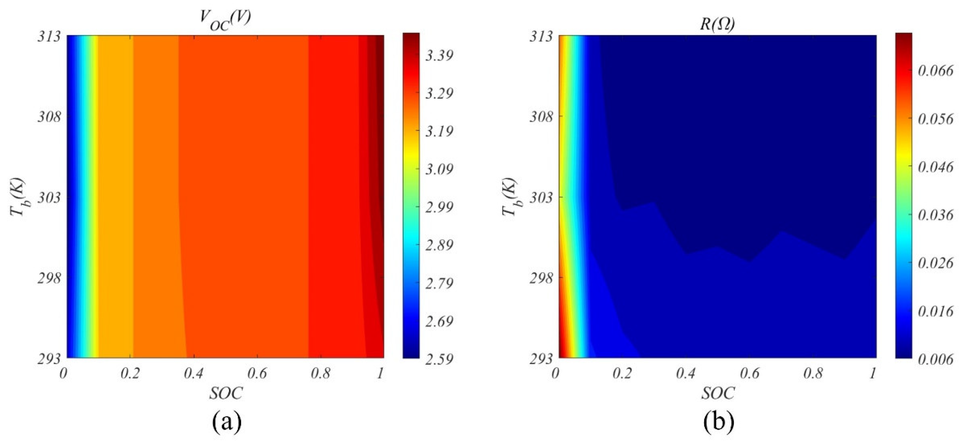
In this study, $V_{OC}$ and $R$ in Equation (24) are calibrated using a contour map based on the battery discharge experiments, as shown in Figure 2.

2.2.2. Pump Model

The pump operation process is simulated using a contour map that includes the input parameters of pump speed, volumetric flow rate, head, and overall efficiency, as shown in Figure 3.

The pump power consumption $P_{pump}$ during operation is calculated using Equation (26).

$$P_{pump}=\frac{\Delta p{q}_{in}}{{\eta }_{pump}}$$

(26)

where, $\Delta p$ represents the static pressure difference between the pump inlet and outlet;$q_{in}$ represents the pump volumetric flow rate; ${\eta }_{pump}$ represents the pump efficiency.

2.2.3. Battery Cooling Valve

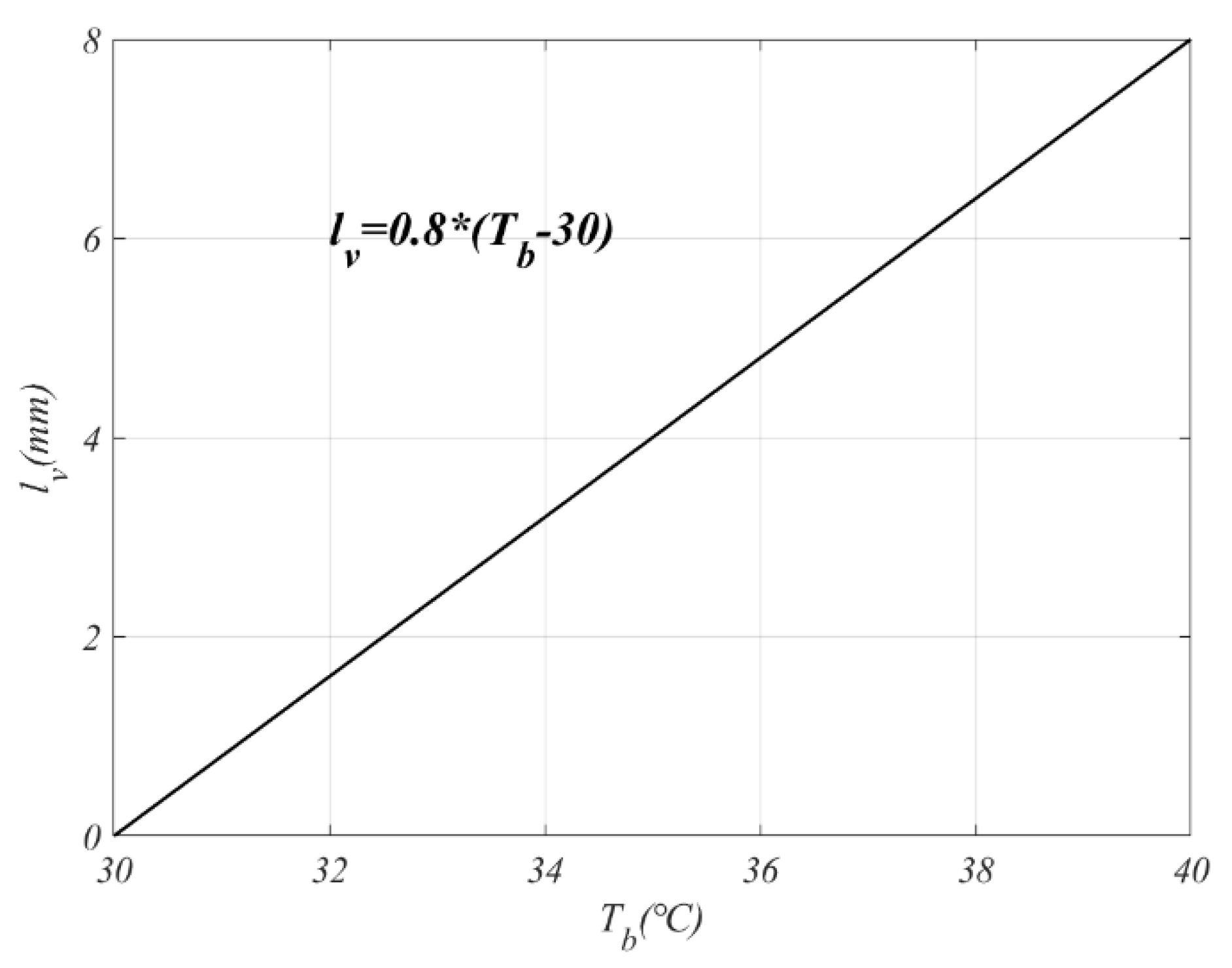
The battery cooling valve used in this study is a proportional valve with a diameter of 8 mm. When $T_b$ is below 30 $°\mathrm{C}$, the valve remains closed, and the chiller in the battery cooling circuit does not need to be coupled with the AC circuit. When $T_b$ exceeds 30 $°\mathrm{C}$, the valve gradually opens to couple the battery cooling circuit with the AC circuit for heat exchange. The relationship between $T_b$ and the battery cooling valve lift $l_v$ is shown in Figure 4.

2.3. Vehicle Dynamic Model

The vehicle dynamic model consists primarily of the electric motor, transmission, differential, and vehicle model, which are all built by the reference model and then combined in GT-Suite. Since the entire vehicle dynamic model is very complex and the research focus of this work is the EVTMS control, we do not describe the whole dynamic model in detail but give the motor model, which is important to calculate the required power provided by the battery. The required power $P_{req}$ of the electric motor is calculated using Equations (27)–(29):

$$T_{qb}=\frac{P_b}{\omega }$$

(27)

$$T_{qi}=T_{qb}+T_{qf}$$

(28)

$$P_{req}=\frac{T_{qi}\omega }{E\left(\omega ,T_{qb}\right)}$$

(29)

where, $P_b$ represents the braking or acceleration power demand; $T_{qb}$ represents the braking or acceleration torque; $T_{qf}$ represents the braking friction torque; $E\left(\omega ,T_{qb}\right)$ represents the electromechanical conversion efficiency.

Other vehicle model parameters used in this paper are shown in

Table 6. Vehicle model parameters.

Parameter	Value
$\mathrm{Curb} \mathrm{weight} (\mathrm{kg}$)	1929
$\mathrm{Full} \mathrm{load} \mathrm{mass} (\mathrm{kg}$)	2335
Wind drag coefficient	0.23
Rolling resistance coefficient	0.01
$\mathrm{Orthographic} \mathrm{area} ({\mathrm{m}}^2$)	3.4
Length · Width · Height $(\mathrm{mm}$)	4750 · 1921 · 1624
$\mathrm{Wheelbase} (\mathrm{mm}$)	2890
$\mathrm{Wheel} \mathrm{tread} (\mathrm{mm}$)	1636

.

The model proposed above is built and combined in GT-Suite, and the final EVTMS is shown in Figure 5.

2.4. Discrete Fluid Model

The fluid variables in the whole EVTMS are mainly solved by 1-dimensional Navier–Stokes equations, including mass, energy, enthalpy and momentum equations as Equations (30)–(33) below.

Mass equation:

$$\frac{dm}{dt}={\displaystyle \sum }_{boundaries}\dot{m}$$

(30)

Energy equation:

$$\frac{d\left(me\right)}{dt}=-p\frac{dV}{dt}+{\displaystyle \sum }_{boundaries}\left(\dot{m}H\right)-h{A}_s\left(T_{fluid}-T_{wall}\right)$$

(31)

Enthalpy equation:

$$\frac{d\left(\rho HV\right)}{dt}=V\frac{dp}{dt}+{\displaystyle \sum }_{boundaries}\left(\dot{m}H\right)-h{A}_s\left(T_{fluid}-T_{wall}\right)$$

(32)

Momentum equation:

$$\frac{d\dot{m}}{dt}=\frac{dpA+{{\displaystyle \sum }}_{boundaries}\left(\dot{m}u\right)-4C_f\frac{\rho u\left|u\right|}{2}\frac{dxA}{D}-K_{p}A\left(\frac{\rho u\left|u\right|}{2}\right)}{dx}$$

(33)

where, $\dot{m}$ is the mass flow rate at the boundary $\dot{m}=\rho Au$; $m$ is mass; $V$ is volume; $p$ is pressure; $\rho$ is density; $A$ is the cross section area; $A_s$ is the heat transfer surface area; $e$ is the total internal energy; $H$ is the enthalpy; $h$ is the heat transfer coefficient; $T_{fluid}$ is the temperature of fluid; $T_{wall}$ is the temperature of wall; $u$ is the velocity on the boundary layer; $C_f$ is the friction coefficient; $K_p$ is the pressure loss coefficient; $D$ is the equivalent diameter; $dx$ is the length of the mass unit in the direction of flow; $dp$ is the pressure difference on $dx$.

The governing equations in the EVTMS are mainly solved by the implicit discrete method based on the principle of virtual work, which is suitable for the pressure pulsation involved in the cooling system and the long-term fluid simulation conditions and has a faster calculation speed, so it will involve the calculation of large time steps. The simulation in this paper ignores the unnecessary pressure pulsation, and the flow calculation time step is solved by Equation (34):

$$\Delta t\propto \frac{V}{A_{e}c}$$

(34)

where, $V$ is the flow volume; $A_e$ is the flow area; $c$ is the velocity of sound.

2.5. Equilibrium Points

In this work, the selected ambient temperature in summer is 40 $°\mathrm{C}$, so the initial temperature of all components in the EVTMS is 40 $°\mathrm{C}$. We also consider the external cabin solar flux input (as shown in Table 3), so when there is no control input and power load, the cabin temperature will slowly rise, which is much closer to the real case.

3. Control Model

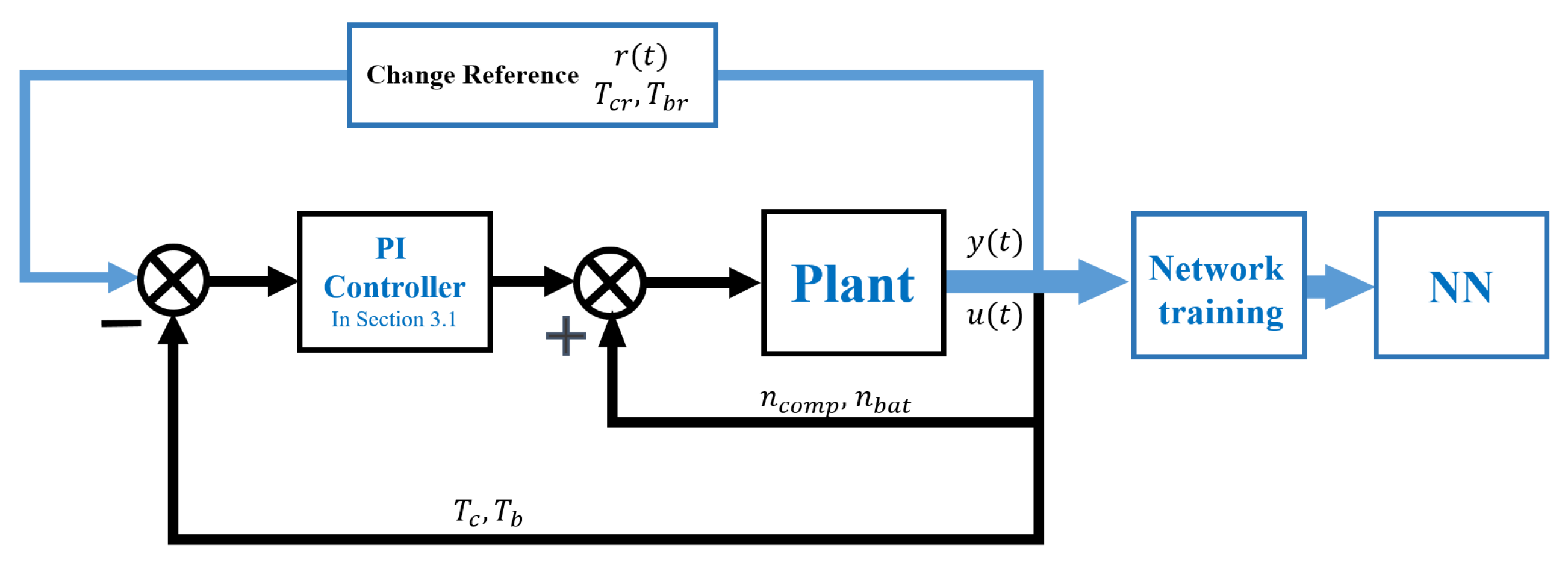
The input–output diagram of the control system is shown in Figure 6. Considering the economic and safety factors, the reference battery temperature $T_{br}$ is set to 35 $°\mathrm{C}$ and the reference cabin temperature $T_{cr}$ is set to the $T_{comfort}$ in Equation (19). The manipulated variables are the pump speed $n_{bat}$ and the compressor speed $n_{comp}$. The main input variables include battery pack temperature $T_b$, cabin temperature $T_c$, vehicle speed $v$, evaporator inlet and outlet temperatures $T_{ein}, T_{eout}$, chiller inlet and outlet temperatures $T_{chin}, T_{chout}$, and battery cooling valve lift $l_v$. The range of the manipulated variables is set as follows:

$$0\le n_{bat}\le 2000; 0\le n_{comp}\le 6000$$

$$-500\le \Delta n_{bat}\le 500; -1000\le \Delta n_{comp}\le 1000$$

3.1. PI Controller

The advantage of proportional (P) controller is timely and rapid, but it will produce residual errors, while the integral (I) controller can eliminate residual errors, but it is not timely. Therefore, this study adds I controller on the basis of P controller to form an incremental parallel PI controller, as shown in Figure 7. However, it should be noted that in this work, two similar PI controllers are used separately, where the first is used for controlling the battery temperature, and the second is used for controlling cabin comfort. The controlled values are the increment of $n_{bat}$ and $n_{comp}$ and the control inputs are the deviations of $T_b$ and $T_c$ from the reference value $T_{br}$, $T_{cr}$, respectively. The control principle is Equations (35)–(37), where $K_p, K_i$ are proportional coefficient and integral coefficient.

$$e\left(t\right)=r\left(t\right)-y\left(t\right)$$

(35)

$$\Delta u\left(t\right)=K_p\left(e\left(t\right)-e\left(t-1\right)\right)+K_{i}e\left(t\right)$$

(36)

$$u\left(t\right)=u\left(t-1\right)+\Delta u\left(t\right)$$

(37)

3.2. Model Predictive Control (MPC)

Model Predictive Control (MPC) has strong robustness and can effectively address issues such as uncertainty and nonlinearity. The control logic diagram is illustrated in Figure 8. MPC consists of three main elements: Prediction Model, Rolling Optimization, and Feedback Control.

• Prediction Model: Based on the current information of the system and future control inputs, the prediction model forecasts the system’s future output;
• Rolling Optimization: This refers to the continuous forward movement in a finite time horizon, where the optimization problem is repeatedly solved;
• Feedback Correction: At each step of rolling optimization, the current system output is compared with the predicted output within the prediction horizon. The error is calculated, and the feedback difference is used for correction.

For each control time step $k$, MPC aims to determine $m$ control increments $\Delta u$, so that the predicted value of the controlled object in the future $p$ steps under its action is as close as possible to the reference value $r$, and meanwhile $\Delta u$ is not too drastic. The objective function is as Equation (38).

$$\min J\left(k\right)={\displaystyle \sum }_{i=1}^p\Vert r\left(k+i|k\right)-\tilde{y}{\left(k+i|k\right)\Vert }_{q_i}^2+{\displaystyle \sum }_{j=1}^m\Vert \Delta u{\left(k+j|k\right)\Vert }_{q_j}^2$$

(38)

where: $k$ represents the current time step; $k+i$ represents the future $i$ step; $q_i$ represents the weight matrix of the tracking error and $q_i=100·I$ in this paper ($I$ represents the identity matrix); $q_j$ represents the weight matrix of the control variable and $q_j=0.06·I$ in this paper; $p$ represents the prediction time horizon; $m$ represents the control time horizon; $r$ represents the reference value; $\Delta u$ represents the change in the manipulated variable.

3.2.1. System Identification Simulation

Black-box model is adopted for system identification for the EVTMS built in Section 2. Compared with grey-box model, black-box model is able to build the state-space function through test data without using much more complex equations of each component, so, in order to obtain useful data for system identification, it is necessary to calibrate the EVTMS through test cycle, as presented in

Table 7. Calibration test.

Time (s)	Speed (km/h) *	${\mathit{n}}_{\mathit{b}\mathit{a}\mathit{t}}$ (RPM)	${\mathit{n}}_{\mathit{c}\mathit{o}\mathit{m}\mathit{p}}$ (RPM)
0–300	0	0	0
300–400		400	1000
400–500		800	2000
500–600		1200	3000
600–700		1600	4000
700–800		2000	5000
800–2600	3 * WLTC	0	0
2600–3320		400	1000
3320–4040		800	2000
4040–4760		1200	3000
4760–5480		1600	4000
5480–6200		2000	5000

* Notice: The vehicle speed is 0 between 0 and 800 s and goes through 3 WLTCs between 800 and 6200 s.

.

The calibration test condition is divided into four stages: 0–300 s, 300–800 s, 800–2600 s and 2600–6200 s, which are mainly used to get the EVTMS performance under different power load and control input. Throughout the calibration test, the pump and compressor speed increased uniformly from the lower limit to the upper limit. Meanwhile, we also give sufficient duration time when the control input changes to allow the system to have sufficient response time. The entire test condition included three WLTC cycles to ensure sufficient external power load. Therefore, these four calibration stages basically include all the operating conditions of the actual EVTMS, which can better reflect the overall characteristics of the system, so as to improve the accuracy of the black-box model. The simulation results are then used to identify the state-space model of the EVTMS.

3.2.2. State-Space Model

The state-space model adopted in this paper is as follows:

$$\left\{\begin{array}{c}x\left(k+1\right)=Ax\left(k\right)+B_{u}u\left(k\right)+B_{d}v\left(k\right)\\ y\left(k\right)=Cx\left(k\right)\end{array}\right.$$

where, $x\left(k\right)$ represents the state variables; $u\left(k\right)$ represents the input variables; $v\left(k\right)$ represents the measurable disturbances; $y\left(k\right)$ represents the output variables; $A$ represents the state matrix; $B_u$ represents the input matrix; $B_d$ represents the measurable disturbance matrix; $C$ represents the output matrix, and the discrete time step is 1 s. It should be noted that the time delay of the EVTMS does not appear in the state-space function as it is difficult to accurately calculate or build the mathematic model of the time delay because of the inherently complex process of the heat transfer, and this issue can be somewhat solved by a method introduced in Section 3.3 below.

In the system identification process, we can freely choose the order of the system state variable $x\left(k\right)$ to achieve more accurate identification performance. Therefore, $x\left(k\right)$ has no practical significance. For the battery cooling circuit, the input variable is $n_{bat}$, the output variable is $T_b$, and the measurable disturbances are $T_{chin}, T_{chout},v,$ $l_v$. For the cabin AC circuit, the input variable is $n_{comp}$, the output variable is $T_c$, and the measurable disturbances are $T_{ein}$, $T_{eout}$, $v$. The simulation result of Section 3.2.1 is used to identify 4-order state-space models using the N4SID method, shown as follows:

Battery cooling circuit:

$$\left(\begin{array}{c}{x}_1\left(k+1\right)\\ x_2\left(k+1\right)\\ x_3\left(k+1\right)\\ x_4\left(k+1\right)\end{array}\right)=A_1\left(\begin{array}{c}{x}_1\left(k\right)\\ x_2\left(k\right)\\ x_3\left(k\right)\\ x_4\left(k\right)\end{array}\right)+B_{u1}{n}_{bat}\left(k\right)+B_{d1}\left(\begin{array}{c}{T}_{chin}\left(k\right)\\ T_{chout}\left(k\right)\\ v\left(k\right)\\ l_v\left(k\right)\end{array}\right)$$

$$T_b\left(k\right)=C_1\left(\begin{array}{c}{x}_1\left(k\right)\\ x_2\left(k\right)\\ x_3\left(k\right)\\ x_4\left(k\right)\end{array}\right)$$

$$A_1=\left[\begin{array}{c}\begin{array}{cc}0.999& -5.67e-4\end{array} \begin{array}{cc}-8.31e-4& 9.55e-4\end{array}\\ \begin{array}{cc}8.54e-3& 0.930\end{array} \begin{array}{cc}-0.0783& 0.0882\end{array}\\ \begin{array}{cc}0.0276& 0.340\end{array} \begin{array}{cc}-0.0356& -0.648\end{array}\\ \begin{array}{cc}0.0214& 0.0563\end{array} \begin{array}{cc}0.919& -0.250\end{array}\end{array}\right]$$

$$B_{u1}=\left[\begin{array}{c}4.72e-8\\ 1.18e-6\\ 7.91e-5\\ -9.63e-7\end{array}\right] B_{d1}=\left[\begin{array}{c}\begin{array}{cc}4.08e-4& -5.80e-5\end{array} \begin{array}{cc}-9.18e-6& -0.0168\end{array}\\ \begin{array}{cc}0.0312& -1.12e-3\end{array} \begin{array}{cc}-4.34e-4& -1.04\end{array}\\ \begin{array}{cc}0.346& -0.0383\end{array} \begin{array}{cc}5.79e-3& 14.9\end{array}\\ \begin{array}{cc}-0.371& 0.0200\end{array} \begin{array}{cc}5.84e-3& 14.6\end{array}\end{array}\right]$$

$$C_1=\left[\begin{array}{cc}-49.1& 0.129\end{array}\begin{array}{cc}8.49e-3& -9.04e-3\end{array}\right]$$

AC circuit:

$$\left(\begin{array}{c}{x}_1\left(k+1\right)\\ x_2\left(k+1\right)\\ x_3\left(k+1\right)\\ x_4\left(k+1\right)\end{array}\right)=A_2\left(\begin{array}{c}{x}_1\left(k\right)\\ x_2\left(k\right)\\ x_3\left(k\right)\\ x_4\left(k\right)\end{array}\right)+B_{u1}{n}_{\mathit{comp}}\left(k\right)+B_{d2}\left(\begin{array}{c}{T}_{\mathit{ein}}\left(k\right)\\ T_{\mathit{eout}}\left(k\right)\\ v\left(k\right)\end{array}\right)$$

$$T_c\left(k\right)=C_2\left(\begin{array}{c}{x}_1\left(k\right)\\ x_2\left(k\right)\\ x_3\left(k\right)\\ x_4\left(k\right)\end{array}\right)$$

$$A_2=\left[\begin{array}{c}\begin{array}{cc}0.996& -7.44e-3\end{array} \begin{array}{cc}-2.78e-4& -4.56e-4\end{array}\\ \begin{array}{cc}-4.00e-3& 0.976\end{array} \begin{array}{cc}-0.0955& 0.0113\end{array}\\ \begin{array}{cc}0.0139& 0.0947\end{array} \begin{array}{cc}0.286& -0.816\end{array}\\ \begin{array}{cc}-0.0141& 0.0474\end{array} \begin{array}{cc}0.857& 0.161\end{array}\end{array}\right]$$

$$B_{u2}=\left[\begin{array}{c}-3.47\mathrm{e}-8\\ 1.85\mathrm{e}-6\\ -4.00e-5\\ -6.29e-5\end{array}\right]{ B}_{d2}=\left[\begin{array}{ccc}1.36\mathrm{e}-5& 6.14\mathrm{e}-6& -8.84\mathrm{e}-7\\ -1.50\mathrm{e}-3& -6.16\mathrm{e}-4& 3.60\mathrm{e}-5\\ -3.70\mathrm{e}-3& -1.81\mathrm{e}-3& -2.21\mathrm{e}-4\\ 0.0195& 8.68\mathrm{e}-3& -7.06\mathrm{e}-4\end{array}\right]$$

$$C_2=\left[\begin{array}{cc}322& -1.15\end{array}\begin{array}{cc}0.145& -0.0852\end{array}\right]$$

3.3. NN-Fuzzy PI Controller

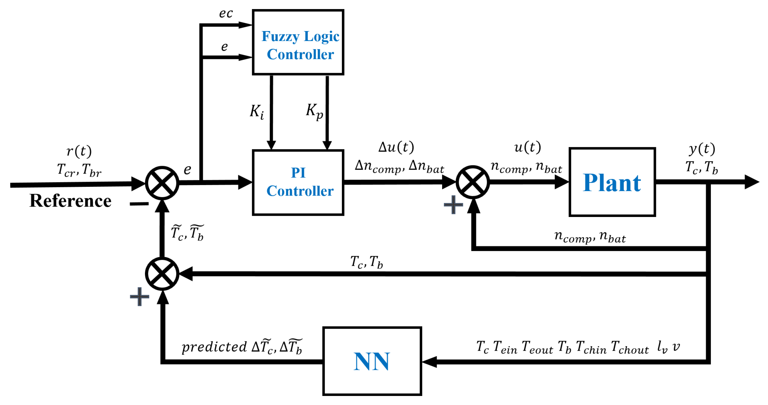
The optimization of the PI controller built in Section 3.1 is performed by incorporating a BP neural network to predict the system variable change at time $k+x$, where $x$ is the prediction time point. The prediction is then used as a feedforward correction in the control loop to mitigate the issues arising from the nonlinearity of the EVTMS and time delay caused by heat transfer. Additionally, a fuzzy controller is also introduced to determine the required $K_p$, $K_i$ values for the PI controller under different output errors. Therefore, the proposed neural network fuzzy PI (NN-Fuzzy PI) controller is illustrated in Figure 9.

3.3.1. BP Neural Network Model

A three-layer BP neural network is employed in this study, as shown in Figure 10. It should be noted that two different BP neural networks with the same structure are used for battery temperature prediction and cabin temperature prediction, respectively. For the battery cooling circuit, $n_{bat}, T_{chin}, T_{chout},v, l_v$ at time $k$ are input layer variables, and the battery temperature change $\widetilde{\Delta T_b}$ at time $k+x$ is output layer variable. For the AC circuit, $n_{comp}, T_{ein},T_{eout}, v$ at time $k$ are input layer variables, while the cabin temperature change $\widetilde{\Delta T_c}$ at time $k+x$ is output layer variable. Neural networks of both battery cooling circuit and AC circuit have 10 neurons in the hidden layer, and the prediction time point is set to $x=10 \mathrm{s}$. The number of hidden layer neurons is the ideal value obtained through trial and error, which can prevent the neural network from underfitting or overfitting.

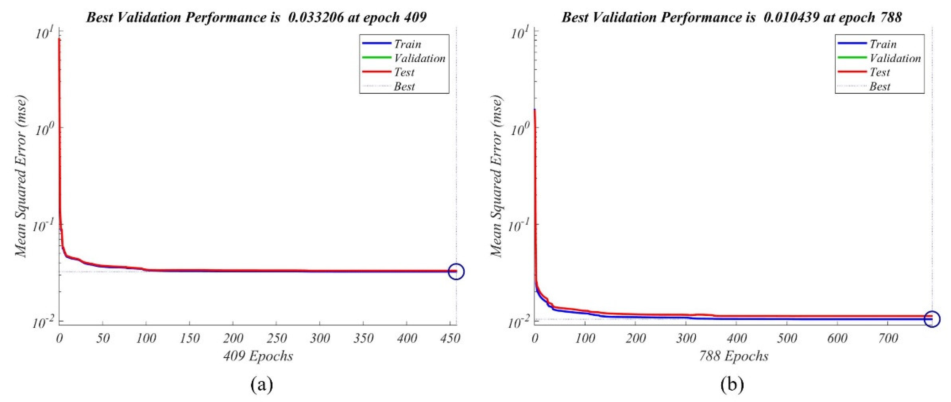
This study performs multiple simulations of the PI controller established in Section 3.1, and the simulation results are used as training samples for neural networks. The training diagram is shown in Figure 11. The training is conducted using the Bayesian regularization method, where the total number of samples is 39,380, with the training set, validation set, and testing set comprising 70%, 15%, and 15%, respectively. The training results are shown in Figure 12, Figure 13 and Figure 14.

3.3.2. Fuzzy PI Controller

Fuzzy control is suitable for solving nonlinear, strong coupling, time-varying and hysteresis problems because it does not need the exact mathematical model and has strong robustness and high tolerance. Thus, it is widely used in industrial applications, such as liquid level, dryer speed and energy storage control [43,44,45].

This study adopts a fuzzy controller combined with the PI controller to form a Fuzzy PI controller, aiming to reduce system oscillations when the deviations are small and ensure sufficient system adjustments when the deviations are large. The input variables of the Fuzzy PI controller are the temperature deviation $e$ between the reference temperature $T_{ref}$ and the actual temperature $T$ and its change rate $ec$. $e$ and $ec$ are defined as Equations (39) and (40):

$$e=T_{ref}-T$$

(39)

$$ec=\frac{de}{dt}$$

(40)

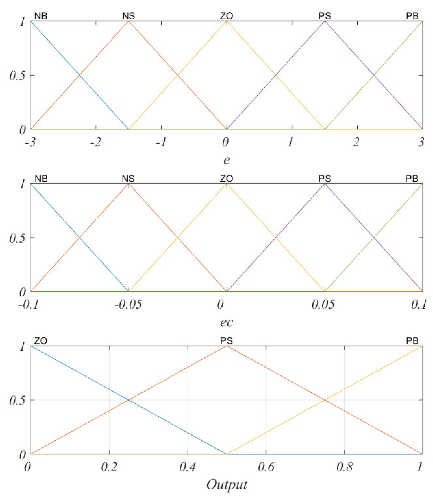
The membership functions of $e$ and $ec$ are set up according to references [46,47]. The symmetrical triangular membership functions shown in Figure 15 are applied to the input and output variables to increase the calculation efficiency.

In the figures, the basic domain and fuzzy domain for $e$ are both set as [−3, 3]. The basic domain and fuzzy domain for $ec$ are both set as [−0.1, 0.1]. Beyond this range, it is treated as a boundary value. Five fuzzy subsets are defined for $e$ and $ec$, with linguistic variables being (NB, NS, ZO, PS, PB). For the output, the basic domain and fuzzy domain for $K_p$ are set as [0, 3000] and [0, 1], respectively. The basic domain and fuzzy domain for $K_i$ are set as [0, 0.01] and [0, 1]. Three fuzzy subsets are defined for the $K_p$, $K_i$, with linguistic variables being (NB, NS, ZO).

This paper adopts the same fuzzy control rules for both $K_p$ and $K_i$, as shown in

Table 8. Control rules of $K_p$, $K_i$.

e ec	NB	NS	ZO	PS	PB
NB	PB	PB	PB	PB	PS
NS	PB	PS	PS	PS	ZO
ZO	PS	ZO	ZO	ZO	PS
PS	ZO	PS	PS	PS	PB
PB	PS	PB	PB	PB	PB

. In the control process, the controller queries the control rules according to $e$ and $ec$. After removing fuzziness, the fuzzy logic system sends the $K_p$, $K_i$ values to the PI controller. This realizes self-adaptation of the PI parameters.

3.4. Controller Parameters

The controller parameters ($K_p, K_i$, control domain $m$, prediction domain $p$, weight coefficient, fuzzy control rules, neural network structure, prediction point, etc.) in Section 3.1, Section 3.2 and Section 3.3 are determined by trial and error. It is relatively simple and does not take much time, which is commonly used in the industry. We first obtain a series of simulation groups by changing controller parameters through the control variable method, and then, compare the simulation results of each control parameter, and finally, summarize the results of the most representative parameters in Section 4.

4. Result and Analysis

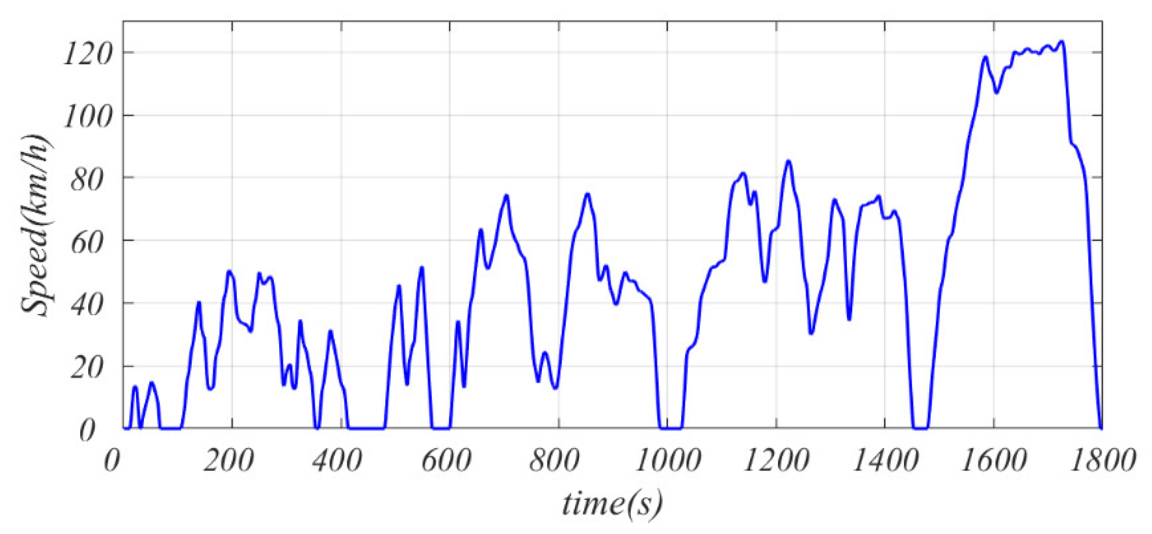
The EVTMS built in Section 2, combined with the controllers built in Section 3, including PI, MPC, and NN-Fuzzy PI controllers, is simulated through a WLTC condition (as shown in Figure 16). Controller parameters are varied to observe their performance. The temperature root-mean-square error (RMSE) ($S$) and its change magnitude ($\Delta S$) are calculated using Equations (41) and (42).

$$S=\frac{1}{N}\sqrt{{\displaystyle \sum }_{i=1}^N{\left(T_i-T_{ref}\right)}^2}$$

(41)

$$\Delta S=S-S_{NN-FuzzyPI}$$

(42)

where, $N$ represents the target calculation time; $T_i$ represents the temperature at time $i$; $T_{ref}$ represents the reference temperature; $S_{NN-FuzzyPI}$ represents the $S$ value of NN-Fuzzy PI controller.

4.1. Battery Pack Temperature Control Effect

Figure 17 shows the control effect of different $K_p$ values on the battery pack temperature $T_b$ and the corresponding pump speed $n_{bat}$ under PI controller. When $K_p$ is relatively small (i.e., the blue line in Figure 17a), the system response is slower, and temperature fluctuations are more pronounced. On the other hand, when $K_p$ is too large, although the fluctuations of $T_b$ decrease, the corresponding $n_{bat}$ increases (i.e., the green line in Figure 17b). Excessive $n_{bat}$ changes may lead to a shortened lifespan of the pump. Therefore, an ideal control scenario for PI controller lies around a $K_p$ value of −300.

Figure 18 shows the control effect of different control and prediction horizons on $T_b$ and the corresponding $n_{bat}$ under MPC. Higher control and prediction horizons can result in better $T_b$ performance at the cost of more pronounced $n_{bat}$ variations (i.e., the green line in Figure 18). The ideal control and prediction horizons are $m=10 \mathrm{s}$ and $p=20 \mathrm{s}$ among the three cases. For lower control and prediction horizons, the $T_b$ performance is poorer because the state-space model cannot accurately predict the future temperature variations of this complex nonlinear system.

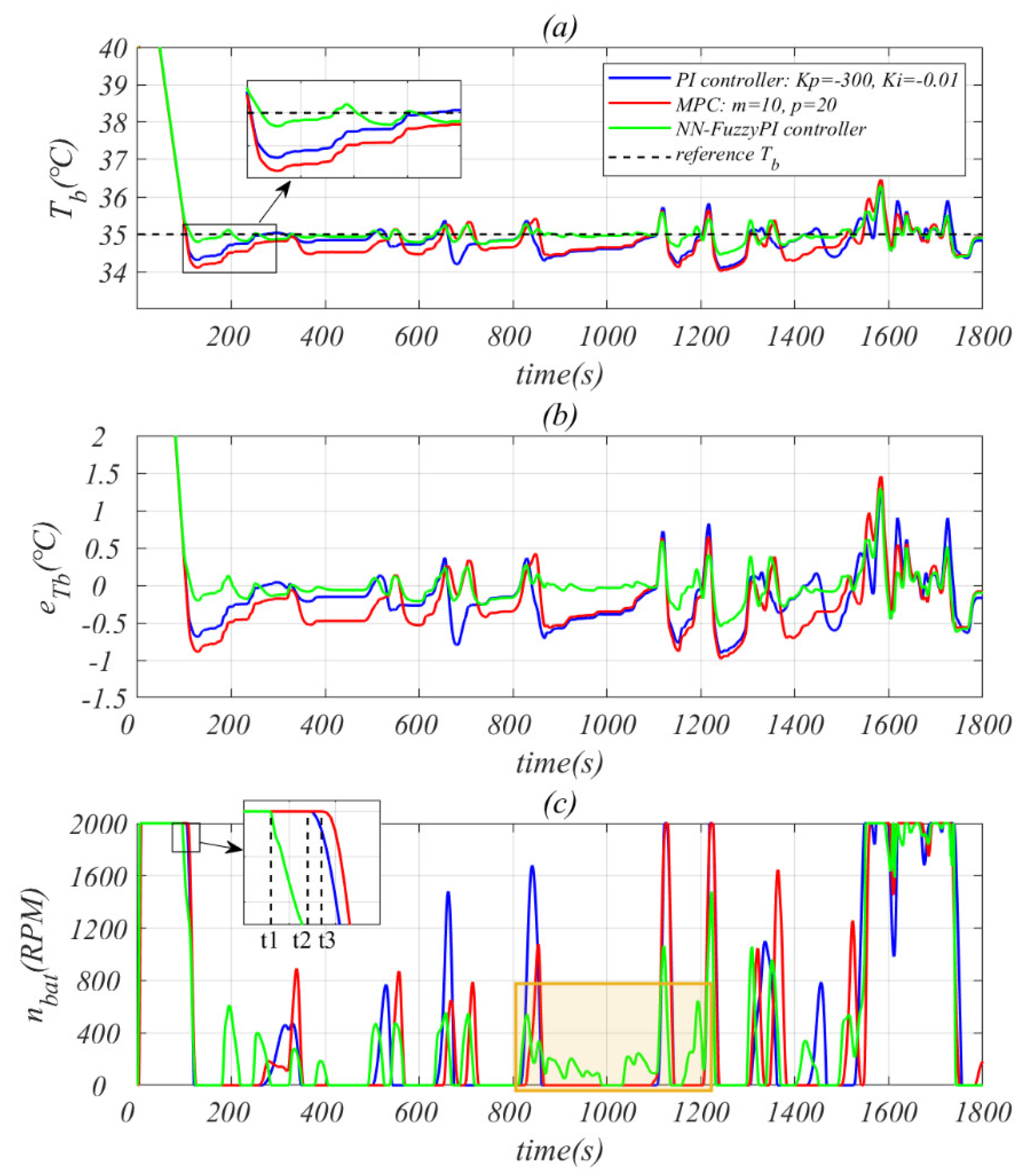
Figure 19 shows the control effect on $T_b$, $e_{Tb}$, and corresponding $n_{bat}$ under PI controller, MPC, and NN-Fuzzy PI controller. Compared to PI controller, MPC does not exhibit obvious advantages in terms of $T_b$ performance, such as the blue and red lines in the black zoomed-in box area near 100–400 s in Figure 19a.

Although both PI controller and MPC can maintain the $e_{Tb}$ within the range of [−1, 1], they have limitations in effectively reducing temperature fluctuations after reaching the target value due to the inherent limitations of the PI and MPC models in describing complex nonlinear systems and the time delay caused by heat transfer. However, by introducing the neural network prediction as feedforward to compensate for the future $T_b$ changes, the $T_b$ fluctuations under NN-Fuzzy PI controller are significantly reduced (i.e., the green line in Figure 19a,b), along with a decrease in the variation amplitude of $n_{bat}$. The NN-Fuzzy PI controller also enables temperature adjustments by preemptively activating or deactivating the pump in response to overshoot caused by the time delay caused by heat transfer in the battery cooling circuit. For example, in Figure 19c,$n_{bat}$ is reduced before $t$ reaching 90 s to prevent excessive battery cooling (i.e., t1 < t2 < t3 in the black zoomed-in box area near 80–120 s), and $n_{bat}$ is relatively lower and more steady in the interval of 800–1200 s instead of a sudden increase (i.e., the yellow box area), resulting in smaller overshoot in the control of $T_b$ after reaching the reference temperature.

Meanwhile, it should be noted that MPC, in principle, should have the best performance with its capability of optimization. However, it is based on the prerequisite of grey-box model instead of the black-box model adopted in this work. So, even though we can freely choose the dimensions of the state-space functions, there are still errors between the established black-box model in MPC and the real one, while the NN-Fuzzy PI controller is directly based on the output of the plant, which is the main reason why MPC does not perform as well as NN-Fuzzy PI controller in this work.

Table 9. RMSE between $T_b$ and $T_{br}$ and the pump energy consumption $W_{pump}$.

Controller	${\mathit{S}}_{\mathit{T}\mathit{b}}$	$\mathbf{\Delta }{\mathit{S}}_{\mathit{T}\mathit{b}}$	$\mathbf{\Delta }$ (%)	${\mathit{W}}_{\mathit{p}\mathit{u}\mathit{m}\mathit{p}}\left(\mathbf{KJ}\right)$	$\mathbf{\Delta }{\mathit{W}}_{\mathit{p}\mathit{u}\mathit{m}\mathit{p}}\left(\mathbf{KJ}\right)$	$\mathbf{\Delta }$ (%)
PI Controller ($K_p=-150, K_i=-0.01)$	0.5845	0.3589	159.1	1.225	0.182	17.45
PI Controller ($K_p=-300, K_i=-0.01)$	0.3873	0.1617	71.68	1.238	0.195	18.70
PI Controller ($K_p=-600, K_i=-0.01)$	0.4264	0.2008	89.01	1.274	0.231	22.15
MPC $\left(m=5, p=10\right)$	0.6158	0.3902	173.0	1.237	0.194	18.60
MPC $\left(m=10, p=20\right)$	0.4571	0.2315	102.6	1.181	0.138	13.23
MPC $\left(m=20, p=40\right)$	0.4647	0.2391	106.0	1.233	0.190	18.22
NN-Fuzzy PI Controller	0.2256	0	0	1.043	0	0

shows the $S_{Tb}$ values between $T_b$ and $T_{br}$ after 100 s as well as the pump energy consumptions $W_{pump}$ under different controllers. It is obvious that the NN-Fuzzy PI controller reaches the lowest $S_{Tb}$ and $W_{pump}$ among all cases. Compared to PI controller, the NN-Fuzzy PI controller reduces $S_{Tb}$ by 70% to 150% and $W_{pump}$ by 17% to 22%; compared to MPC, it reduces $S_{Tb}$ by 106% to 173% and $W_{pump}$ by 13% to 18%.

4.2. PMV Control Effect

Figure 20 shows the control effect of different $K_p$ values on $PMV$ and the corresponding compressor speed $n_{comp}$ under PI controller. In comparison to its control on $T_b$ (i.e., Figure 17a), the PI controller cannot achieve an ideal performance on $PMV$, which is mainly because the cabin model has the external solar flux inputs (the solar flux value in Table 3). And PI controllers cannot accurately capture the influence of unmeasurable external inputs, resulting in $PMV$ only being confined to the range of [−1, 1]. As $K_p$ increases, the system becomes more sensitive to $PMV$ fluctuations, leading to faster attainment of local peaks in $PMV$ and $n_{comp}$ troughs. For example, the peak arrival times follow the order $\mathrm{t}1<\mathrm{t}2<\mathrm{t}3$ in the black zoomed-in box area near 700–800 s in Figure 20b. Meanwhile, a higher $K_p$ value will also cause larger $PMV$ fluctuations according to Figure 21a. An ideal control scenario for PI control lies around a $K_p$ value of −150.

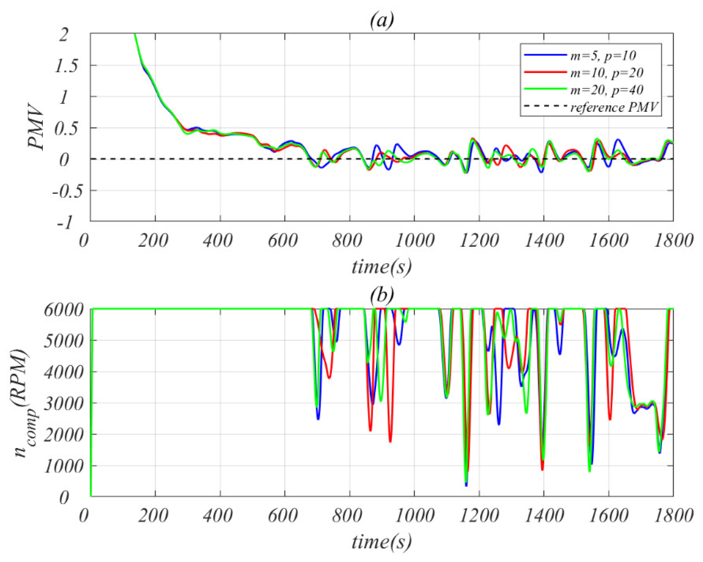
Figure 21 shows the control effect of different control horizons and prediction horizons on $PMV$ and the corresponding $n_{comp}$ under MPC. MPC can confine $PMV$ within the range of [−0.25, 0.25], providing a comfortable experience for the driver, and meanwhile adjust $n_{comp}$ reasonably based on the current $PMV$ value. However, due to unmeasurable disturbances such as the solar flux, MPC still struggles to effectively reduce the fluctuations after reaching the reference $PMV$. Although increasing the prediction horizon can slightly reduce the fluctuations, it also leads to significant and frequent changes in $n_{comp}$ (i.e., the green line in Figure 21). Therefore, the ideal control and prediction horizons are $m=10 \mathrm{s}$ and $p=20 \mathrm{s}$ among the three cases, taking both $PMV$ fluctuation reduction and avoiding excessive and frequent changes in $n_{comp}$ into consideration.

Figure 22 shows the control effect on $PMV$, $e_{PMV}$, and corresponding $n_{comp}$ under PI controller, MPC, and NN-Fuzzy PI controller. It is obvious that MPC can reduce $PMV$ fluctuations compared to PI controller (i.e., the blue and red lines in Figure 22a,b). However, due to their limitations in describing complex nonlinear systems, MPC and PI controllers can only limit $e_{PMV}$ to the range [−0.3, 0.3]. On the other hand, by incorporating a predictive feedforward of $T_c$, the NN-Fuzzy PI controller can significantly reduce the $e_{PMV}$ to a range of [−0.1, 0.1] (i.e., the green line in Figure 22a,b), where the driver can hardly perceive any temperature changes.

Furthermore, by comparing the changes in $n_{comp}$, it can be seen that the NN-Fuzzy PI controller effectively anticipates the time delay caused by heat transfer and reduces the overshoot by lowering $n_{comp}$ before reaching the reference $PMV$. For instance, in the interval of 1600–1800 s (i.e., the yellow box area in Figure 22c), $n_{comp}$ of the PI controller exhibits only one low peak (i.e., the blue line in Figure 22c), while MPC maintains $n_{comp}$ around 3000 RPM (i.e., the red line in Figure 22c), and the NN-Fuzzy PI controller varies $n_{comp}$ between 2000 and 5000 RPM to compensate for the fluctuations in $PMV$ (i.e., the green line in Figure 22c).

Table 10. RMSE between $PMV$ and $PM{V}_r$ and the compressor energy consumption $W_{comp}$.

Controller	${\mathit{S}}_{\mathit{P}\mathit{M}\mathit{V}}$	$\mathbf{\Delta }{\mathit{S}}_{\mathit{P}\mathit{M}\mathit{V}}$	$\mathbf{\Delta }$ (%)	${\mathit{W}}_{\mathit{c}\mathit{o}\mathit{m}\mathit{p}}\left(\mathbf{KJ}\right)$	$\mathbf{\Delta }{\mathit{W}}_{\mathit{c}\mathit{o}\mathit{m}\mathit{p}}\left(\mathbf{KJ}\right)$	$\mathbf{\Delta }$ (%)
PI Controller ($K_p=-75, K_i=-0.01)$	0.2135	0.1287	151.8	3251.9	81.8	2.580
PI Controller ($K_p=-150, K_i=-0.01)$	0.1760	0.0912	107.6	3269.5	99.4	3.136
PI Controller ($K_p=-300, K_i=-0.01)$	0.2239	0.1391	164.0	3270.2	100.1	3.158
MPC $\left(m=5, p=10\right)$	0.1343	0.0495	58.4	3245.3	75.2	2.372
MPC $\left(m=10, p=20\right)$	0.1200	0.0352	41.5	3232.9	62.8	1.981
MPC $\left(m=20, p=40\right)$	0.1221	0.0373	43.9	3253.9	83.8	2.643
NN-Fuzzy PI Controller	0.0848	0	0	3170.1	0	0

presents the values of $S_{PMV}$ after 600 s as well as the compressor energy consumptions $W_{comp}$ under different controllers. MPC outperforms PI controller in terms of $S_{PMV}$ and $W_{comp}$ and NN-Fuzzy PI controller exhibits the lowest $S_{PMV}$ and $W_{comp}$ among all the cases. Compared to the PI controller, the NN-Fuzzy PI controller reduces $S_{PMV}$ by 107% to 164% and $W_{pump}$ by 2.58% to 3.16%; compared to MPC, it reduces $S_{PMV}$ by 43% to 58% and $W_{pump}$ by 1.98% to 2.68%.

4.3. Performance of Neural Network Feedforward

The effectiveness of neural network feedforward (NN feedforward) in the Fuzzy PI controller has been proved in Section 4.1 and Section 4.2. To further explore its performance in different controllers, we add it to the MPC controller to form neural network-MPC (NN-MPC), as shown in Figure 23, where the NNs are the same as the NNs used in the NN-Fuzzy PI controller.

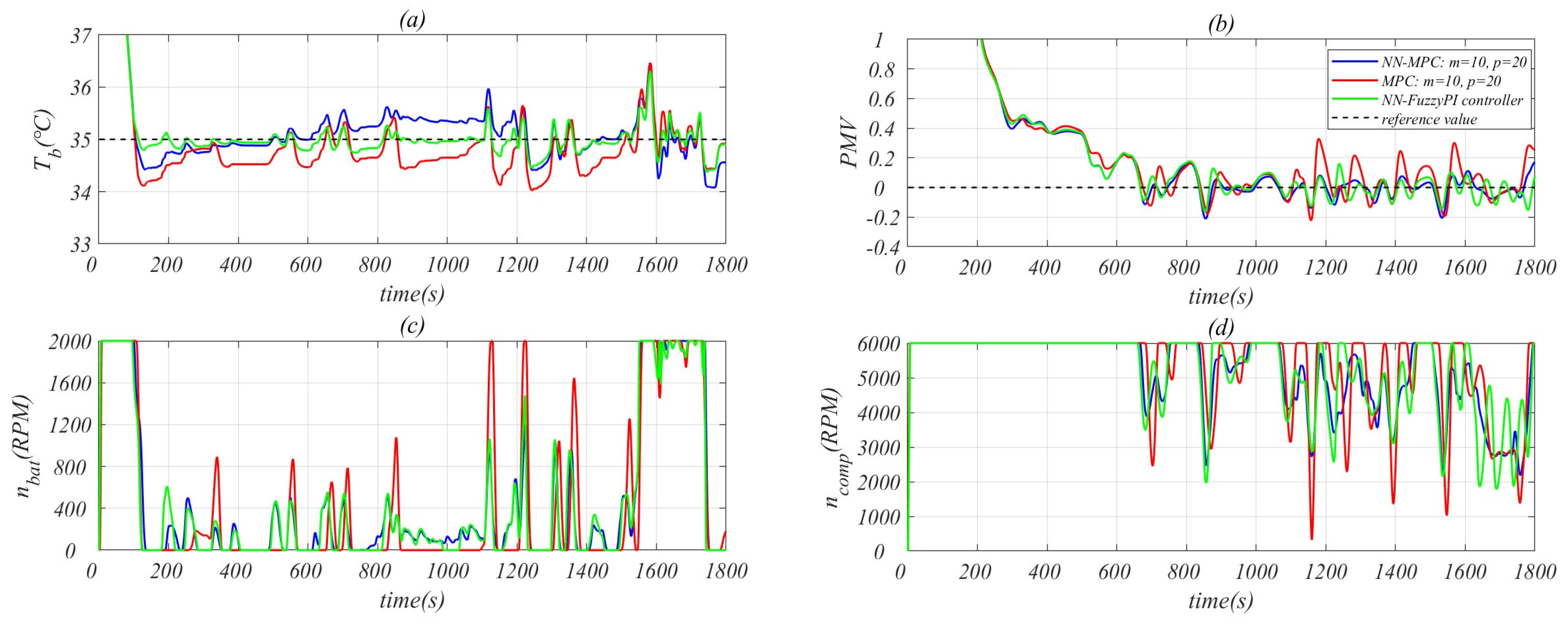
Figure 24 shows the control effect of $T_b$ and $PMV$ as well as corresponding pump and compressor speed under the NN-MPC, MPC and NN-Fuzzy PI controller. It is obvious that compared with MPC (i.e., the red line in Figure 24), after adding the NN prediction as feedforward, $T_b$ and $PMV$ fluctuations are significantly reduced (i.e., the blue line in Figure 24). Although there is a gap of $T_b$ with the reference value in the range of 700–1000 s, the overall performance and the pump speed curve are much closer to those of the NN-Fuzzy PI controller. Meanwhile, $PMV$ fluctuations of NN-MPC are even lower than the NN-Fuzzy PI controller, which proves the effectiveness of neural network feedforward in MPC.

Table 11. RMSE between $T_b$ and $T_{br}$ and the pump energy consumption $W_{pump}$.

Controller	${\mathit{S}}_{\mathit{T}\mathit{b}}$	$\mathbf{\Delta }{\mathit{S}}_{\mathit{T}\mathit{b}}$	$\mathbf{\Delta }$ (%)	${\mathit{W}}_{\mathit{p}\mathit{u}\mathit{m}\mathit{p}}\left(\mathbf{KJ}\right)$	$\mathbf{\Delta }{\mathit{W}}_{\mathit{p}\mathit{u}\mathit{m}\mathit{p}}\left(\mathbf{KJ}\right)$	$\mathbf{\Delta }$ (%)
MPC $\left(m=10, p=20\right)$	0.4571	0.2315	102.6	1.181	0.138	13.23
NN-MPC $\left(m=10, p=20\right)$	0.3651	0.1395	61.8	1.085	0.042	4.03
NN-Fuzzy PI Controller	0.2256	0	0	1.043	0	0

presents the $S_{Tb}$ values after 100 s and pump energy consumption $W_{pump}$ under MPC, NN-MPC and NN-Fuzzy PI controller. Compared with MPC, $S_{Tb}$ and $W_{pump}$ of NN-MPC are significantly reduced by 40.8% and 9.2%, respectively, but they are still higher than those of NN-Fuzzy PI controller.

Table 12. RMSE between $PMV$ and $PM{V}_r$ and the compressor energy consumption $W_{pump}$.

Controller	${\mathit{S}}_{\mathit{P}\mathit{M}\mathit{V}}$	$\mathbf{\Delta }{\mathit{S}}_{\mathit{P}\mathit{M}\mathit{V}}$	$\mathbf{\Delta }$ (%)	${\mathit{W}}_{\mathit{c}\mathit{o}\mathit{m}\mathit{p}}\left(\mathbf{KJ}\right)$	$\mathbf{\Delta }{\mathit{W}}_{\mathit{c}\mathit{o}\mathit{m}\mathit{p}}\left(\mathbf{KJ}\right)$	$\mathbf{\Delta }$ (%)
MPC $\left(m=10, p=20\right)$	0.1200	0.0352	41.5	3232.9	62.8	1.981
NN-MPC $\left(m=10, p=20\right)$	0.0819	−0.0029	−3.4	3166.7	−3.4	−0.107
NN-Fuzzy PI Controller	0.0848	0	0	3170.1	0	0

presents the $S_{PMV}$ values after 600 s and compressor energy consumption $W_{comp}$. NN-MPC can achieve the same or even better control performance of $PMV$ than NN-Fuzzy PI controller. Compared with MPC, $S_{PMV}$ and $W_{comp}$ can even be reduced by 44.9% and 2.1%, respectively, by NN-MPC.

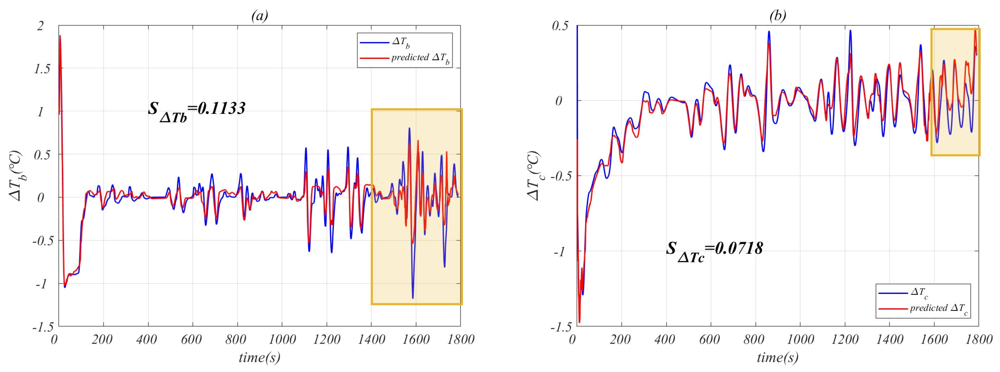
Meanwhile, the neural networks’ predicted temperature deviations $\widetilde{\Delta T_b}$ and $\widetilde{\Delta T_c}$ compared to the actual simulation output $\Delta T_b$ and $\Delta T_c$ are shown in Figure 25. It can be seen that the neural networks can accurately capture the temperature trends. Although there are some areas with larger prediction errors (i.e., the yellow box areas in Figure 25), indicating the effect of neural networks is limited within this range (i.e., the ultra-high-speed segment in WLTC), $S_{\Delta Tb}$ and $S_{\Delta Tc}$ are 0.1133 $°\mathrm{C}$ and 0.0718 $°\mathrm{C}$, respectively, which are small enough to provide effective feedforward compensation for the control of $T_b$ and $T_c$.

According to the above analysis, the effectiveness of neural network feedforward in MPC is verified. Therefore, the neural network feedforward plays a crucial role in improving the performance of different controllers and reducing energy consumption.

5. Conclusions

This study presents a one-dimensional EVTMS simulation model under summer conditions, considering both the battery pack temperature and the cabin comfort, and eventually, the performance of different controllers on this model is compared. The following conclusions are drawn:

Compared to MPC, PI controller shows weaker performance in controlling the AC circuit because of the unmeasurable external disturbances;

1.

Under WLTC condition, the NN-Fuzzy PI controller can accurately predict the nonlinear and time delay characteristics of the EVTMS and provide advanced feedforward to the system, resulting in better control performance and lower energy consumption compared to PI controller and MPC;

2.

The $T_b$ fluctuations under NN-Fuzzy PI controller are within the range of [−0.5, 0.5], while the $PMV$ fluctuations are within the range of [−0.1, 0.1];

3.

Compared to PI controller, the NN-Fuzzy PI controller reduces $S_{Tb}$ by 70% to 150% and $W_{pump}$ by 17% to 22%; compared to MPC, it reduces $S_{Tb}$ by 106% to 173% and $W_{pump}$ by 13% to 18%;

4.

Compared to PI controller, the NN-Fuzzy PI model reduces $S_{PMV}$ by 107% to 164% and $W_{comp}$ by 2.58% to 3.16%; compared to MPC, it reduces $S_{PMV}$ by 43% to 58% and $W_{comp}$ by 1.98% to 2.68%;

5.

When NN feedforward is added to MPC, $S_{Tb}$, $S_{PMV}$ and the energy consumption are also significantly reduced, which indicates the effectiveness of NN feedforward in different controllers.

Furthermore, due to the adaptive capabilities of neural networks, the dynamic prediction performance can become more accurate with increased training data. However, this study also has limitations and optimization space:

• Factors that may affect the EVTMS performance, such as the battery arrangement and consistency, are not considered, which can be further studied by CFD simulation to establish a more accurate battery model;
• Some algorithms, such as nonlinear model predictive control (NMPC), genetic algorithms (Gas) and particle swarm optimization (PSO), can be used to control all variables inside EVTMS instead of only pump and compressor speed;
• Parameters and hyperparameters in the controllers can be further optimized;
• The robustness and performance of controllers under heating conditions in the winter can be further tested.

Future research can be carried out according to the above aspects. It is hoped that the conclusions of this study can assist TMS engineers in choosing better control strategies and building advanced EVTMS.

References

1. Lu, L.; Han, X.; Li, J.; Hua, J.; Ouyang, M. A review on the key issues for lithium-ion battery management in electric vehicles. J. Power Sources 2013, 226, 272–288. [Google Scholar] [CrossRef]
2. Hosen, M.S.; Youssef, R.; Kalogiannis, T.; Van Mierlo, J.; Berecibar, M. Battery cycle life study through relaxation and forecasting the lifetime via machine learning. J. Energy Storage 2021, 40, 102726. [Google Scholar] [CrossRef]
3. Sun, P.; Bisschop, R.; Niu, H.; Huang, X. A Review of Battery Fires in Electric Vehicles. Fire Technol. 2020, 56, 1411. [Google Scholar] [CrossRef]
4. Yang, T.; Yang, N.; Zhang, X.; Li, G. Investigation of the thermal performance of axial-flow air cooling for the lithium-ion battery pack. Int. J. Therm. Sci. 2016, 108, 132–144. [Google Scholar] [CrossRef]
5. Bandhauer, T.M.; Garimella, S.; Fuller, T.F. A Critical Review of Thermal Issues in Lithium-Ion Batteries. J. Electrochem. Soc. 2011, 158, R1–R25. [Google Scholar] [CrossRef]
6. Liu, H.; Wei, Z.; He, W.; Zhao, J. Thermal issues about Li-ion batteries and recent progress in battery thermal management systems: A review. Energy Convers. Manag. 2017, 150, 304–330. [Google Scholar] [CrossRef]
7. Wang, Q.; Jiang, B.; Li, B.; Yan, Y. A critical review of thermal management models and solutions of lithium-ion batteries for the development of pure electric vehicles. Renew. Sustain. Energy Rev. 2016, 64, 106–128. [Google Scholar] [CrossRef]
8. Yokoyama, A.; Osaka, T.; Imanishi, Y.; Sekiya, S. Thermal Management System for Electric Vehicles. SAE Int. J. Mater. Manuf 2011, 4, 1277–1285. [Google Scholar] [CrossRef]
9. Kiss, T.; Chaney, L.; Meyer, J. A New Automotive Air Conditioning System Simulation Tool Developed in MATLAB/Simulink. SAE Int. J. Passeng. Cars-Mech. Syst. 2013, 6, 826–840. [Google Scholar] [CrossRef]
10. Kiss, T.; Lustbader, J. Comparison of the Accuracy and Speed of Transient Mobile A/C System Simulation Models. SAE Int. J. Passeng. Cars-Mech. Syst. 2014, 7, 739–754. [Google Scholar] [CrossRef]
11. Kiss, T.; Lustbader, J.; Leighton, D. Modeling of an Electric Vehicle Thermal Management System in MATLAB/Simulink. In Proceedings of the SAE 2015 World Congress & Exhibition, Detroit, MI, USA, 21–23 April 2015. [Google Scholar]
12. Lee, S.; Chung, Y.; Kim, S.; Jeong, Y.; Kim, M.S. Investigation on the performance enhancement of electric vehicle thermal management system utilizing floating loop with finite heat exchanger size. Energy Convers. Manag. 2022, 255, 115265. [Google Scholar] [CrossRef]
13. Yang, Q.; Zeng, T.; Zhang, C.; Zhou, W.; Xu, L.; Zhou, J.; Jiang, P.; Jiang, S. Modeling and simulation of vehicle integrated thermal management system for a fuel cell hybrid vehicle. Energy Convers. Manag. 2023, 278, 116745. [Google Scholar] [CrossRef]
14. Shah, S.; Vijay, D.; Lehocky, M. Thermal Management of Electrified Vehicle by Means of System Simulation. In Proceedings of the Thermal Management Systems Conference 2020, Berlin, Germany, 21–22 January 2020. [Google Scholar]
15. Dong, Y.Q.; Wu, H.; Zhou, J.; Ding, Y.; Wang, X.; Xu, S. Designing and Evaluating the Integrated Thermal Management System of a Plug-in Parallel Hybrid Electric Vehicle. In Proceedings of the SAE 2020 Vehicle Electrification and Autonomous Vehicle Technology Forum, Shanghai, China, 3–4 December 2020. [Google Scholar]
16. Deng, L.; Li, S.; Tang, X.; Yang, K.; Lin, X. Battery thermal- and cabin comfort-aware collaborative energy management for plug-in fuel cell electric vehicles based on the soft actor-critic algorithm. Energy Convers. Manag. 2023, 283, 116889. [Google Scholar] [CrossRef]
17. Asef, A.; Chitsaz, I.; Madan, N. Modeling and total cost optimization of battery thermal management system in a hybrid electric vehicle. J. Energy Storage 2022, 52 Pt A, 104844. [Google Scholar] [CrossRef]
18. Wang, Z.R.; Huang, L.P.; He, F. Design and analysis of electric vehicle thermal management system based on refrigerant-direct cooling and heating batteries. J. Energy Storage 2022, 51, 104318. [Google Scholar] [CrossRef]
19. Cen, J.; Jiang, F. Li-ion power battery temperature control by a battery thermal management and vehicle cabin air conditioning integrated system. Energy Sustain. Dev. 2020, 57, 141–148. [Google Scholar] [CrossRef]
20. Yasaman, M.; Ahmad, M.; Nasser, L.A. Battery Thermal Management of Electric Vehicles: An Optimal Control Approach. In Proceedings of the ASME 2015 Dynamic Systems and Control Conference, Columbus, OH, USA, 28–30 October 2015. [Google Scholar]
21. Chong, Z.; Fei, L.; Hua, Z.; Jing, S.; Chris, M.C. A Real-Time Battery Thermal Management Strategy for Connected and Automated Hybrid Electric Vehicles (CAHEVs) Based on Iterative Dynamic Programming. IEEE Trans. Veh. Technol. 2018, 67, 8077–8084. [Google Scholar]
22. Min, H.; Zhang, Z.; Sun, W.; Min, Z.; Yu, Y.; Wang, B. A thermal management system control strategy for electric vehicles under low-temperature driving conditions considering battery lifetime. Appl. Therm. Eng. 2020, 181, 115944. [Google Scholar] [CrossRef]
23. Shen, W.; Wang, N. Simulation and Control of Battery Thermal Management System for Electric Vehicle. In Proceedings of the Vehicle Electrification and Powertrain Diversification Technology Forum, Beijing, China, 23–24 August 2022. [Google Scholar]
24. Şefkat, G.; Özel, M.A. Experimental and numerical study of energy and thermal management system for a hydrogen fuel cell-battery hybrid electric vehicle. Energy 2022, 238, 121794. [Google Scholar] [CrossRef]
25. Wang, H.; He, F.; Ma, L. Experimental and modeling study of controller-based thermal management of battery modules under dynamic loads. Int. J. Heat Mass Transf. 2016, 103, 154–164. [Google Scholar] [CrossRef]
26. Bauer, S.; Suchaneck, A.; León, F.P. Thermal and energy battery management optimization in electric vehicles using Pontryagin’s maximum principle. J. Power Sources 2014, 246, 808–818. [Google Scholar] [CrossRef]
27. Zhang, Z.; Min, H.; Yu, Y.; Cao, Q.; Li, M.; Yan, K. An optimal thermal management system heating control strategy for electric vehicles under low-temperature fast charging conditions. Appl. Therm. Eng. 2022, 207, 118123. [Google Scholar] [CrossRef]
28. Xie, Y.; Liu, Z.; Liu, J.; Li, K.; Zhang, Y.; Wu, C.; Wang, P.; Wang, X. A Self-learning intelligent passenger vehicle comfort cooling system control strategy. Appl. Therm. Eng. 2020, 166, 114646. [Google Scholar] [CrossRef]
29. Yasaman, M.; Nasser, L.A. MPC-based battery thermal management controller for Plug-in hybrid electric vehicles. In Proceedings of the IEEE 2017 American Control Conference (ACC), Seattle, WA, USA, 24–26 May 2017. [Google Scholar]
30. Vermillion, C.; Jing Sun Butts, K. Predictive Control Allocation for a Thermal Management System Based on an Inner Loop Reference Model—Design, Analysis, and Experimental Results. IEEE 2011, 19, 772–781. [Google Scholar] [CrossRef]
31. Tao, X.W.; Wagner, J. Cooling Air Temperature and Mass Flow Rate Control for Hybrid Electric Vehicle Battery Thermal Management. In Proceedings of the ASME 2014 Dynamic Systems and Control Conference, San Antonio, TX, USA, 22–24 October 2014. [Google Scholar]
32. Tao, X.; Zhou, K.; Ivanco, A.; Wagner, J.R.; Hofmann, H.; Filipi, Z. A Hybrid Electric Vehicle Thermal Management System—Nonlinear Controller Design. In Proceedings of the SAE 2015 World Congress & Exhibition, Detroit, MI, USA, 21–23 April 2015. [Google Scholar]
33. Lopez-Sanz, J.; Ocampo-Martinez, C.; Alvarez-Florez, J.; Moreno-Eguilaz, M.; Ruiz-Mansilla, R.; Kalmus, J.; Graeber, M.; Lux, G. Nonlinear Model Predictive Control for Thermal Management in Plug-in Hybrid Electric Vehicles. IEEE Trans. Veh. Technol. 2015, 66, 3632–3644. [Google Scholar] [CrossRef]
34. Lopez-Sanz, J.; Ocampo-Martinez, C.; Alvarez-Florez, J.; Moreno-Eguilaz, M.; Ruiz-Mansilla, R.; Kalmus, J.; Graeber, M.; Lux, G. Thermal Management in Plug-In Hybrid Electric Vehicles: A Real-Time Nonlinear Model Predictive Control Implementation. IEEE Trans. Veh. Technol. 2016, 66, 7751–7760. [Google Scholar] [CrossRef]
35. Ma, Y.; Ding, H.; Mou, H.; Gao, J. Battery thermal management strategy for electric vehicles based on nonlinear model predictive control. Measurement 2021, 186, 110115. [Google Scholar] [CrossRef]
36. Liu, Y.; Zhang, J. Self-adapting J-type air-based battery thermal management system via model predictive control. Appl. Energy 2020, 263, 114640. [Google Scholar] [CrossRef]
37. García-Morales, J.; Cervantes-Bobadilla, M.; Hernández-Pérez, J.A.; Saavedra-Benítez, Y.I.; Adam-Medina, M.; Guerrero-Ramírez, G.V. Inverse artificial neural network control design for a double tube heat exchanger. Case Stud. Therm. Eng. 2022, 34, 102075. [Google Scholar] [CrossRef]
38. Fanger, P.O. Thermal Comfort; Danish Technical Press: Copenhagen, Denmark, 1970. [Google Scholar]
39. Farzaneh, Y.; Tootoonchi, A.A. Controlling automobile thermal comfort using optimized fuzzy controller. Appl. Therm. Eng. 2008, 28, 1906–1917. [Google Scholar] [CrossRef]
40. Jang, M.S.; Koh, C.D.; Moon, I.S. Review of thermal comfort design based on PMV/PPD in cabins of Korean maritime patrol vessels. Build. Environ. 2007, 42, 55–61. [Google Scholar] [CrossRef]
41. Toftum, J.; Jorgensen, A.S.; Fanger, P.O. Upper limits for indoor air humidity to avoid uncomfortably humid skin. Energy Build. 1998, 28, 1–13. [Google Scholar] [CrossRef]
42. Atmaca, I.; Yigit, A. Predicting the effect of relative humidity on skin temperature and skin wittedness. J. Therm. Biol. 2006, 31, 442–452. [Google Scholar] [CrossRef]
43. Euzébio, T.A.M.; Ramirez, M.A.P.; Reinecke, S.F.; Hampel, U. Energy Price as an Input to Fuzzy Wastewater Level Control in Pump Storage Operation. IEEE Access 2023, 11, 93701–93712. [Google Scholar] [CrossRef]
44. Júnior, M.P.; da Silva, M.T.; Guimarães, F.G.; Euzébio, T.A.M. Energy savings in a rotary dryer due to a fuzzy multivariable control application. Dry. Technol. 2022, 40, 1196–1209. [Google Scholar] [CrossRef]
45. Gopi, B.; Ramesh, G.; Logeshwaran, J. The Fuzzy Logical Controller Based Energy Storage and Conservation Model to Achieve Maximum Energy Efficiency In Modern 5G Communication. ICTACT J. Commun. Technol. 2022, 13, 2774–2779. [Google Scholar]
46. Mann, G.K.I.; Hu, B.-G.; Gosine, R.G. Analysis of direct action fuzzy PID controller structures. IEEE Trans. Syst. Man Cybern. Part B 1999, 29, 371–388. [Google Scholar] [CrossRef]
47. Wang, Y.; Jin, Q.; Zhang, R. Improved fuzzy PID controller design using predictive functional control structure. ISA Trans. 2017, 71 Pt 2, 354–363. [Google Scholar] [CrossRef]
Figure 1. Battery cooling circuit and cabin AC circuit.
Energies 17 00009 g001
Figure 2. Contours of S O C , T b and battery parameters (a) open voltage; (b) internal resistance.
Energies 17 00009 g002
Figure 3. Contours of head, volumetric flow rate and pump parameters (a) speed; (b) efficiency.
Energies 17 00009 g003
Figure 4. T b vs. l v .
Energies 17 00009 g004
Figure 5. Electric vehicle thermal management system.
Energies 17 00009 g005
Figure 6. Input and output of the control system.
Energies 17 00009 g006
Figure 7. PI controller structure.
Energies 17 00009 g007
Figure 8. MPC structure.
Energies 17 00009 g008
Figure 9. NN-Fuzzy PI controller structure.
Energies 17 00009 g009
Figure 10. BP neural network structure.
Energies 17 00009 g010
Figure 11. Neural network training diagram.
Energies 17 00009 g011
Figure 12. Error histogram (a) Δ T b ; (b) Δ T c .
Energies 17 00009 g012
Figure 13. NN results for the complete dataset (a) Δ T b ; (b) Δ T c .
Energies 17 00009 g013
Figure 14. Epoch graphic (a) Δ T b ; (b) Δ T c .
Energies 17 00009 g014
Figure 15. Membership functions of e, ec and output.
Energies 17 00009 g015
Figure 16. WLTC condition.
Energies 17 00009 g016
Figure 17. PI controller results (a) T b ; (b) n b t .
Energies 17 00009 g017
Figure 18. MPC results (a) T b ; (b) n b a t .
Energies 17 00009 g018
Figure 19. Results of PI controller, MPC, NN-Fuzzy PI controller (a) T b ; (b) e T b ; (c) n b a t .
Energies 17 00009 g019
Figure 20. PI controller results (a) P M V ; (b) n c o m p .
Energies 17 00009 g020
Figure 21. MPC results (a) P M V ; (b) n c o m p .
Energies 17 00009 g021
Figure 22. Results of PI controller, MPC, NN-Fuzzy PI controller (a) P M V ; (b) e P M V ; (c) n c o m p .
Energies 17 00009 g022
Figure 23. NN-MPC structure.
Energies 17 00009 g023
Figure 24. Results of NN-MPC, MPC, NN-Fuzzy PI controller (a) T b ; (b) P M V ; (c) n b a t ; (d) n c o m p .
Energies 17 00009 g024
Figure 25. Neural network output and actual simulation output (a) Δ T b ; (b) Δ T c .
Energies 17 00009 g025