1. Introduction
The advanced metering infrastructure in electrical systems (AMI) allows for the collection of consumption data from users and circuits at multiple levels of electrical distribution networks, with a resolution that can reach hours or minutes, in contrast to classic meters, which are limited to daily or monthly data. The data in an AMI network is generated by smart meters located in consumption areas and connected to an IT infrastructure that stores the data and enables real-time modifications to the distribution of energy through the power grid. In this way, the inclusion of AMI within an electrical distribution grid allows for a more precise and optimized management of distribution, giving rise to what is known as a “smart grid”. In addition to leveraging the real-time management and operation of the grid, the continuous monitoring of users’ energy consumption enables the development of a range of data-driven applications. These applications include demand characterization (which allows for a much more detailed identification of how energy is consumed by users), analysis of the variables that have an impact on energy consumption (such as location, climate, elevation, and whether the user is a resident or a business), and the development of demand flexibility scenarios or the introduction of new sources or consumers. These new functionalities require support by constant analysis of the data flow between the servers that manage the data and the devices in the field.
This paper is intended as a continuation of the work completed in recent years by some of its authors. The previous work [
1] presents two main results. The first is a database with processed records from power consumption measurements in Colombia between 2017 and 2021. Each sample in the dataset contains the energy consumption levels of a specific user in a specific moment, as well as information regarding the type of user and geographical location. Each user is registered among three possible classes: residential, commercial, or industrial. To this database, a segmentation model using the k-means clustering method was applied in order to identify the load profiles for different types of users. This set of load profiles (of which almost 40 were obtained) is the second main result of the previous work.
In this paper, this previous work is expanded by taking into account a new series of databases that contain data from electrical substations. The data, collected by three network operators, can be used as the basis for different analyses of energy consumption registered at a higher level of the electrical distribution grid. The broader scope of the substations allows us to focus on the consumption of a small area (a neighborhood, a small town, or a countryside area), rather than on individual users. The substations data is processed, and each substation is then compared to the clusters of users to locate the load profiles that have more affinity with each substation; thus, the clusters can be used as a mean to understand the behavior of the users linked to the substation. Although the grid operators routinely know which users are linked to a particular substation, depending of their geographic location, load profiles can be seen as a more accurate characterization of the users, allowing for a more in-depth analysis of their behavior.
The structure of this document is as follows:
Section 2 gives a brief overview of related work regarding smart grids and the most common applications in the field, including several case studies.
Section 3 provides a detailed view of the features of the substations data and its processing and presents the details of the proposed methodology, including the previous work on segmentation and our new contributions, i.e., the identification of the user load profiles more related to each substation and the characterization of the user profiles connected to each substation. The results of this process for data from three different grid operators are presented in
Section 4, and the conclusions of our work are presented in
Section 5.
2. Background and Related Work
New paradigms such as the smart grid (SG) have become popular research topics in response to the growing demand for electrical energy and the increasing awareness of environmental concerns associated with the use of renewable energies. Smart grids (SG) have proven their ability to meet the requirements of the electrical system by integrating unconventional energy generation methods alongside traditional fossil fuel sources. In order to ensure the optimal performance of these networks, real-time information from smart meters (SM) is essential. Smart meters enable the measurement of electrical energy consumption, current levels, voltage, and power factors, providing valuable insights into the flow of energy to and from the network [
2].
The adoption of this type of metering technology has witnessed significant global growth, driven by policies such as Resolution 40,072 of 2018 by the Colombian Ministry of Mines and Energy. This resolution establishes the objectives and legal framework for the implementation of an advanced measurement infrastructure (AMI) in this country. Its goal is to connect 95% of urban users and 50% of populated and rural areas by 2030. In contrast, smart meters account for a significant proportion of the total meters installed in developed countries. For instance, in Europe, it was estimated that by 2020, 72% of installed meters would be smart meters. Similarly, in the United States, the percentage of smart electric meters installed in 2021 reached 72% of the total [
3,
4].
Given that smart meters are capable of collecting data at minute intervals, the volume of information generated is substantial. As a result, the utilization of research and data analysis tools becomes crucial for the effective planning and implementation of electrical networks. Consequently, numerous authors have focused on extracting meaningful insights from the raw data obtained from smart meters or advanced metering infrastructure (AMI). These research endeavors can be categorized into the following groups:
2.1. Load Forecasting
Load forecasting is a pivotal concern in electrical power systems, ensuring the uninterrupted and properly regulated supply of energy in terms of current and voltage. Notably, the evolving demand and power generation landscape in recent years has given rise to distinct consumption patterns among end users [
5]. Factors such as the integration of electric vehicle charging infrastructure and the widespread adoption of distributed generation technologies like solar panels and windmills have contributed to these changes. Moreover, the shift towards remote work due to the COVID-19 pandemic has also impacted energy consumption patterns [
6,
7].
The prediction of electrical energy consumption can be categorized into four distinct time frames: very short-term load forecasting (VSTLF), short-term load forecasting (STLF), medium-term load forecasting (MTLF), and long-term load forecasting (LTLF). VSTLF focuses on predicting consumption within seconds and minutes. Common methods employed in VSTLF include moving average models, neural networks, and genetic algorithms, among others [
5]. As demonstrated by Ref. [
8], they proposed a short-term demand prediction model for the industrial sector utilizing long short-term memory networks (LSTM). The approach involves exploratory data analysis and preprocessing stages before feeding the data into three groups of LSTM networks. Each of these networks undergoes pruning using the proposed BRSB technique (bagging, random subspace, and boosting), enabling the combination of their respective results to effectively generate load forecasts.
Short-term load forecasting (STLF) plays a crucial role in predicting demand within a timeframe ranging from a few minutes to a few hours. It provides essential information for the day-to-day operations of the system, enabling effective load management. To achieve a better understanding of load behavior in this time interval, researchers incorporate various external variables such as weather conditions, seasonality, and day type [
5]. An example of such research is the work presented by Ref. [
9], in which the employ the Prophet algorithm, developed by Facebook, is employed to identify load parameters and forecast demand for subsequent hours up until the following day.
Medium-term load forecasting (MTLF) is typically employed to predict load patterns spanning from a few days to several months. In a study by Ref. [
10], an innovative approach utilizing an auto-hiding neural network (AENN) was implemented to forecast monthly energy consumption. This process involves compressing the hourly consumption dataset and subsequently feeding it into the AENN, which assigns weights to each prediction made. By aggregating these forecasts, a comprehensive and accurate estimate of future energy consumption is obtained.
Long-term load forecasting (LTLF) is employed to predict load patterns spanning from weeks to years. In addition to historical load variables, external factors, such as weather conditions, the number of clients, and the socioeconomic status of the users, are commonly considered. For instance, in a study by Ref. [
11], a neural network model was used to estimate the total energy consumption in Malaysia. The model utilized input data including the estimated population, the number of users, demand peaks, and per capita consumption. By incorporating these variables, the neural network model provided accurate forecasts of long-term energy demand in the country.
2.2. Load Profile Identification
The rise in household appliances and electronic devices utilized for everyday tasks has led to a notable surge in residential energy consumption, contributing significantly to the overall global demand for electricity. Notably, households account for 36% of the energy demand in the United States and 25% in Europe [
12]. Consequently, extensive research has been conducted to mitigate residential energy consumption, including initiatives such as load monitoring, which are aimed at promoting energy efficiency and conservation in residential settings.
Load monitoring (LM) aims to measure the electrical energy consumption and usage patterns of household appliances. In the literature, LM can be classified into three categories: intrusive load monitoring (ILM), non-intrusive load monitoring (NILM), and other methods. ILM implementation can be costly, as it requires installing individual meters for each appliance in the home. Additionally, it may pose challenges in terms of connectivity due to the large number of devices involved. To address these issues, the NILM methodology, which estimates the individual consumption of electrical appliances by employing disaggregation algorithms on the aggregate consumption data, has been investigated. NILM can further be categorized into three types: machine learning (ML), pattern matching (PM), and single-channel source separation (SS) methods [
12]. For instance, in Ref. [
13], a non-intrusive load monitoring (NILM) method, incorporating appliance usage patterns (AUP), is proposed to enhance the performance of active load identification and forecasting. In the initial stage, the AUPs for a specific residence are learned using a standard NILM algorithm based on spectral decomposition. Subsequently, the obtained AUPs are utilized to bias the a priori probabilities of the devices through a fuzzy system. The method was tested on two standard databases containing real household measurements from the U.S. and Germany, where an improvement in the estimation of the active load was observed.
2.3. Indicator Prediction
Indicators play a crucial role in evaluating the performance, quality, and efficiency of an electrical system. They serve as a basis for making informed decisions, often referred to as data-driven decisions. These indicators can range from the status of individual system nodes or components to the saturation or overload levels of transformers. For instance, in the study conducted by Ref. [
14], a data-driven indicators model is employed to manage an electrical network at the University of Campinas, Brazil. The model utilizes an autoencoder LSTM (long short-term memory) neural network to predict voltage and current imbalances in the system nodes, as well as the level of transformer overload, thus providing valuable indicators for effective operation.
2.4. Demand Response
Currently, the rapid growth in energy demand has sparked increasing interest in alternative sources. Smart grids (SG) can help integrate unconventional energy sources. Furthermore, the incorporation of new technologies like advanced metering infrastructure (AMI) in SG allows for communication between consumers and producers, which can help reduce energy costs. In the context of SG, demand response (DR) is used to mitigate peaks in electricity consumption, also known as the power peak-to-average ratio (PAR), based on real-time pricing (RTP) [
15]. DR integrates price incentive programs to change the consumption patterns of end-users, achieving the stability and balance of energy resources while providing economic efficiency to network stakeholders. The general idea is to raise energy prices during peak demand periods to incentivize users to shift their consumption to off-peak hours or times of low demand. However, user response can create new peaks by increasing demand during off-peak hours. This problem can result from traditional methods of peak demand reduction. Therefore, alternative methods have been proposed, such as real-time pricing (RTP), time-of-use pricing (ToU), and critical peak pricing (CPP), with RTP and ToU being the most widely used. RTP is a policy in which energy prices vary over short time periods, typically hours, taking into account the current cost of energy production. On the other hand, ToU pricing reflects a tariff structure, in which energy prices vary in intervals ranging from hours to days or weeks. The latter is preferred by both network operators and consumers [
16].
2.5. Loss Detection
Energy losses can be classified into two categories: technical losses and non-technical losses. Among the non-technical losses, the primary concern is energy theft. This illicit activity typically involves bypassing the energy meter, manipulating meter readings, or hacking into the meter [
17]. Energy theft poses a significant problem that impacts the profitability of energy companies worldwide. Annually, these companies experience over USD 96 billion in lost profits due to non-technical losses, with theft being the major contributing factor. To provide some perspective, sub-Saharan Africa alone accounts for a staggering 50% of stolen energy, according to the World Bank. Moreover, in 2015, Indian companies suffered losses of USD 16.2 billion, Brazilian companies lost USD 10.5 billion, and Russian companies experienced USD 5.1 billion in losses [
18].
Apart from causing revenue losses, electricity theft has direct and negative consequences on the stability and reliability of electricity grids. It leads to overloads on distribution networks, increases the risk of electric shocks, and raises the probability of network failures. Furthermore, it can impact the price of energy as network operators increase their rates to compensate for the losses, thereby affecting all regular customers as well [
18].
As a result, research has been conducted to develop methods for detecting this type of illicit behavior. In a study by Zhou et al. [
19], they demonstrate how early warnings of anomalous behaviors, potentially indicating energy theft, can be generated using logistic regression analysis. The proposed method consists of three stages: data preprocessing, data augmentation, and data classification. In the data preprocessing step, interpolation and data cleaning techniques are applied to fill in missing values and remove erroneous ones. The data augmentation step utilizes the kernel density estimator (KDE) and the Monte Carlo method to generate new data. Finally, in the data classification step, the datasets are fed into a convolutional neural network (CNN) model to identify instances of electricity theft.
2.6. Fault Detection
In recent years, there has been a significant increase in the deployment of smart meters in electricity networks. However, the utilization of the information provided by these meters for fault detection purposes remains low. Surprisingly, despite 81% of public service companies in the United States having implemented smart meters, only 16% of fault alerts are derived from these devices. Conversely, 26% of the alerts originate from SCADA systems, while 58% are generated through user calls. These statistics underscore the underutilization of smart meters and highlight the untapped potential for further development in this area [
20].
In their study, Mortensen et al. [
20] propose a fault localization method for power distribution systems that utilizes multivariate process monitoring based on principal component analysis (PCA). This method combines fault detection and fault diagnosis techniques and relies solely on aggregated smart meter data, typically collected for billing purposes. To enhance these attributes, the authors employ feature engineering. The output of the method is a prioritized list of component tags indicating the components most likely affected by an outage. The effectiveness of the method is demonstrated using real data from a Danish power distribution system, accurately identifying affected medium voltage transformers and low voltage radials, as well as providing reliable indications of impacted electrical boxes. Integration with a geographic information system (GIS) enables the provision of coordinates for the affected components. Notably, the authors emphasize the method’s ability to avoid false positives.
2.7. Voltage Control
Traditionally, voltage stability has been maintained by regulating the impedance of the power system at the transmission level. However, voltage instability can also be addressed at the end-user side by enabling them to provide controllable real and reactive power. This possibility has become more viable with the increasing adoption of distributed energy resources (DER) and controllable loads at the grid’s edge [
21]. An example of a DER is a photovoltaic system equipped with four-quadrant smart inverters, which can generate both real and reactive power while maintaining control. Additionally, controllable loads, such as heating, ventilation, and air conditioning (HVAC) systems, can adjust their consumption in response to demand response programs, thereby contributing to voltage control efforts.
The authors of Ref. [
21] investigate the feasibility and challenges of implementing voltage control at the grid’s edge. They focus on the voltage monitoring and control function for smart meters and analyze its impact on communication and energy distribution systems. In terms of voltage monitoring, the authors develop a simulation platform using GridLAB-D and ns-3 to assess the effects of incorporating voltage measurements into smart meter readings. They also evaluate strategies to mitigate timeout errors and packet drops at the communication layer. It is important to note that most existing systems were primarily designed for transmitting energy-related information, rather than for the monitoring and control of voltage levels.
Regarding voltage control, the authors of Ref. [
21] propose a voltage stability control scheme that utilizes the voltage stability margin as the control objective, deviating from the conventional voltage magnitude approach. The proposed scheme leverages the advanced metering infrastructure and distributed energy resources (DER) already in place, requiring minimal additional costs. The authors conclude that integrating the voltage monitoring and control function into smart meters has the potential to address voltage stability issues at the “last mile” of the grid, providing a promising solution.
2.8. Price Prediction
In recent decades, many countries have implemented electricity market deregulation, aiming to reduce energy prices through competition. This shift has created an electric power market in which producers and buyers engage in price negotiations, similar to those common with other commodities. As a result, understanding the demand and price of energy becomes crucial in the electricity market. Accurate price prediction empowers participants to better plan their offers regarding the daily energy markets, effectively managing risks and maximizing profits. Notably, even a 1% improvement in load forecast error can yield significant savings, potentially reaching up to USD 300,000 annually for a maximum load of 1 gigawatt (GW). When price forecasting is factored in, the estimated savings can double, reaching approximately USD 600,000 per year [
22].
Consequently, numerous studies have been conducted to predict energy prices, both in the short and long term. Many of these studies leverage big data tools and machine learning techniques to forecast the value of electrical energy. For instance, in Ref. [
23], a dual model is proposed for short-term price prediction. The model combines an LSTM network with a LightGBM model, demonstrating improved prediction performance compared to using either model alone. In Ref. [
24], an optimized neural network incorporating an evolutionary algorithm is applied. The weights and thresholds of the backpropagation neural network are optimized using a differential evolutionary algorithm. The resulting neural network is then employed to test the electricity market. The authors conclude that their proposed model exhibits high stability and accuracy regarding price prediction.
3. Proposed Methodology
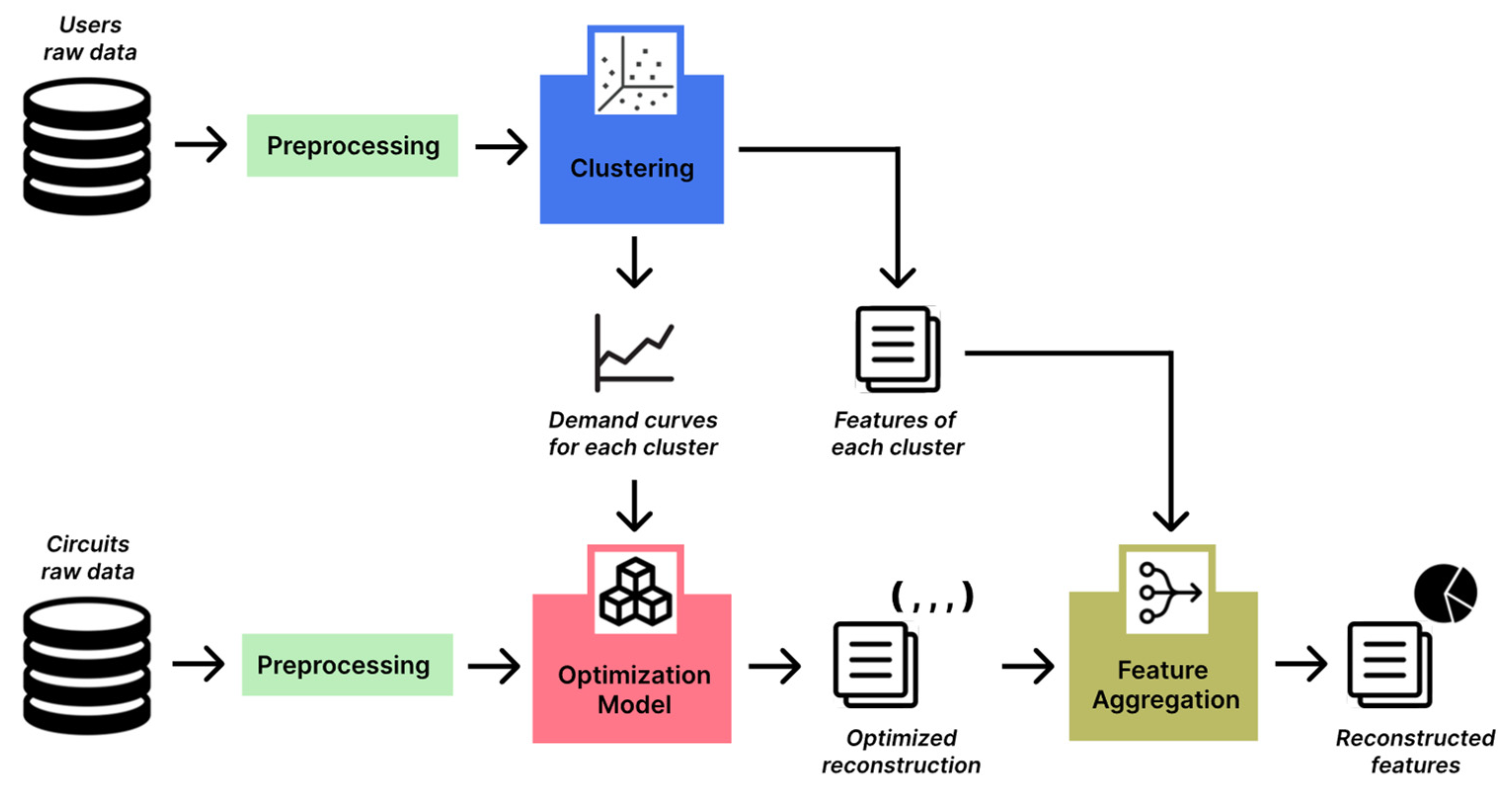
The main contribution of this paper is the design and implementation of a methodology that receives as input both data from electrical end users (consumers) and data from electrical substations, returning a characterization of substation consumption in terms of user load profiles. An overview of the architecture of our methodology can be seen in
Figure 1.
The methodology operates in two distinct pathways. The first of these paths operates on data from users: the data related to each user is pre-processed in order to find its load profile, a unique curve comprising the 24 h of the day showing the average daily consumption of the user over a year. The load profiles from all users are then passed to a clustering algorithm that splits them into distinct clusters of load profiles. Each of the clusters is represented by its prototypical curve (the mean of the profiles of all users in the clusters) and a series of features of the users that compose the cluster (in particular, how many of them are labeled as residential, commercial or industrial users). The details of this pipeline have been previously established and developed in Ref. [
1], including the data collection, filtering, and feature selection; the application of k-means as the selected clustering algorithm; and the obtention of the final results.
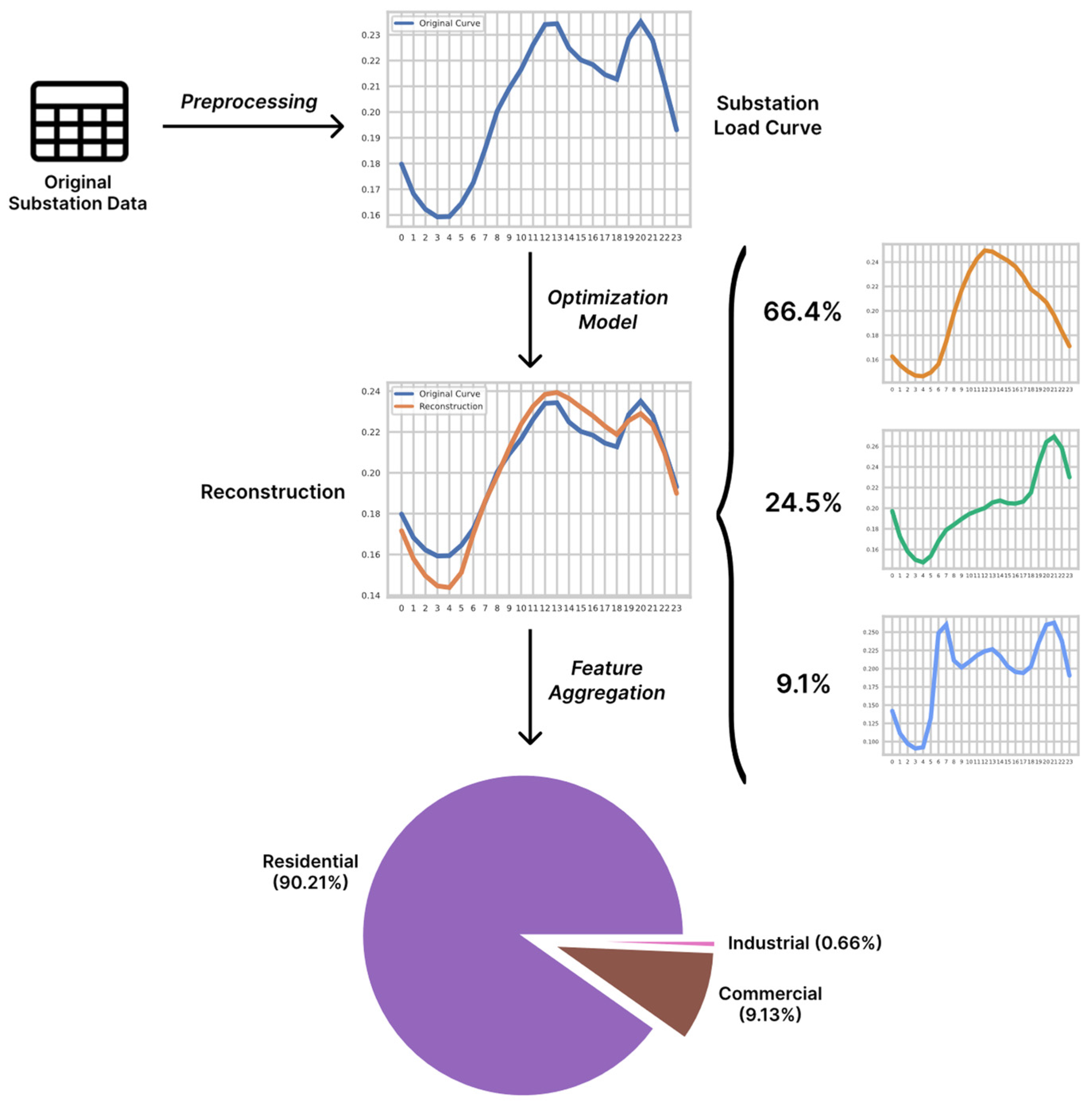
The second path concerning the data from substations is a novel contribution presented in this paper. The load profiles of the substations are built in a similar manner as performed previously, by averaging their daily consumptions over a year. Then, the load profile of each substation is introduced into an optimization model that uses the prototypical curves of the clusters to approximate the composition of the substation consumption in terms of the clusters, building a reconstruction of the original substation curve created from the weighted contributions of each cluster. In this way, the consumption at the substation can be modeled as the combination of multiple profiles of consumptions from the users that depend on it, and some of them will contribute more than others, depending on each case. This means that the output of the model is a set of weights that quantify the contribution of each user profile (or cluster) to the total consumption of the substation. Finally, using all these weights, the features of the clusters can be aggregated in order to understand the features of the users that make up the consumption of the substation. Since we know the specific characteristics of the users in each cluster, we can average them through their weights, giving more importance to the clusters with the largest contributions. An example of the application of this second pipeline to a specific substation can be seen in
Figure 2.
In summary, the methodology consists of three main stages.
The user data is processed to obtain an average consumption curve associated with each user. The curves of all users are transformed into datapoints on which a clustering algorithm (k-means) is applied to obtain a set of groups or clusters with distinct behaviors. Each cluster is then represented by the average curve of all the users that make it up, and also contains the proportions of the different types of users and their geographical distribution.
The substations are also represented by their average consumption curves. For each one, a model is applied that attempt to determine how much each cluster contributes to the substation by analyzing the similarity between curves through an optimization model. If the average curve of a cluster has a high similarity with that of the substation, it is assumed that this cluster has a higher contribution in this substation.
Once the contribution of the clusters has been quantified, the characteristics of the substation (specifically, its composition in terms of types of users) are approximated by considering the types of users in each cluster. The proportions of all types of users in the substation are obtained by taking the proportions of the clusters and averaging them, based on the contributions of the clusters.
Next, we delve into the stages that make up the second pipeline, indicating the steps needed to process the substation data, showing an exploratory analysis of the substations limited to years and months, presenting the method of determining a suitable approximation to the substations data, and providing the manner in which to combine this approximation with information from the clusters in order to determine the unknown properties of the substation in terms of the properties of the users.
3.1. Preprocessing of Substations Data
Data Collection. The collection of data was performed through a formal request to three grid operators in Colombia. The electrical substation databases were provided by the operators, in four different files. Each operator handled its own data formats, so a different treatment for each operator was required. The data was received in four CSV files, and the main features of these files are presented in
Table 1. Some of the files contained information on reactive and capacitive power measurements; for the purposes of the analyses performed there, only active power data were taken into account.
Data Cleaning. The first step in processing the data was to standardize all the database registers so that each register contained the information of a single hourly measurement at a single substation. Although these changes were performed slightly differently for any database file, all of them were given the following structure. Each register contains an identifier of the substation (a unique substation code assigned by each operator), the date of the measurement (day, month, year), the hour of the measurement (with values from zero to 23), and the measured value of active energy in kilowatts per hour (kWh).
After the reordering, many of these registers showed null energy values. To deal with these registers, the null values were replaced by the average of the non-zero readings for the same substation in the same hour, only in cases where the null registers were less than half of the total registers for the substation. If more than half of the registers for a substation had null values, the substation was discarded.
Curve Obtention. The behavior of each substation was modeled through a curve that shows the average daily behavior of consumption in the substation. Formally, a curve consists of a list of 24 values in which each value corresponds to measurements for each hour of the day. This list can be plotted with the hours on the
x-axis and the values on the
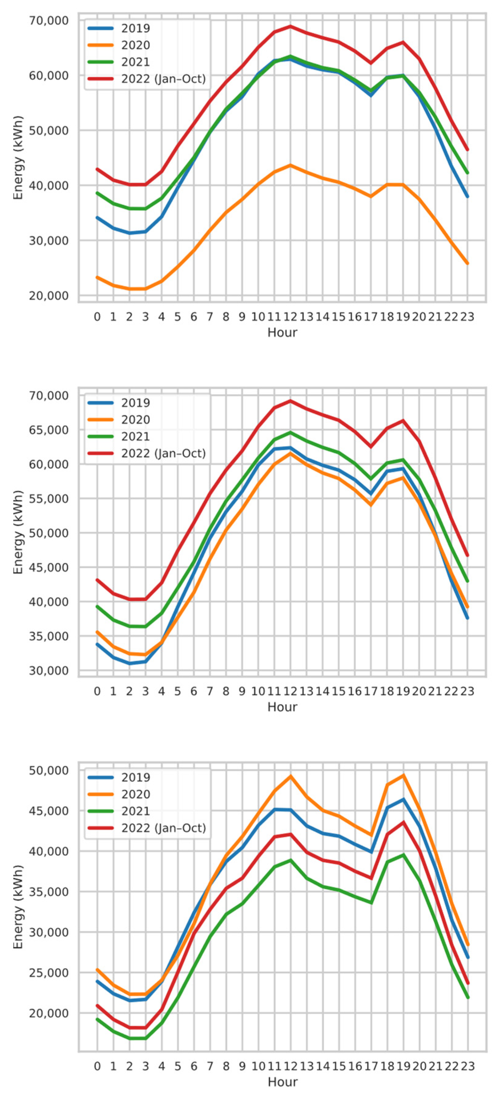
y-axis. The curve for each substation was built by taking all the registers of each hour and finding the average of the measurements. That is, the first value of the curve (hour zero) was found by averaging all registers of the substations taken in hour zero; the second value was found by averaging all the registers taken in hour one, and so on. It was decided to create one curve per year, i.e., each substation has several curves associated with it, in which each curve summarizes all the data for a particular year. Given the temporal scope of our data (see
Table 1), it is possible to observe the variations in electricity demand caused by the restrictions related to COVID-19 that were applied in Colombia in 2020. In some cases, the restrictions caused a significant decrease in consumption; in other cases, the decrease was smaller, or there was even an increase in consumption. However, the load profiles tend to maintain a very similar geometry over the years. Some examples of the changes between 2019 and 2022 are shown in
Figure 3.
All the substation curves used in the following sections of the paper correspond to 2021, since data from this year are available for all operators, and the consumption at that moment was less affected by the COVID-19 restrictions ordered in Colombia in 2020.
3.2. Reconstruction and Aggregation
Every curve (either for a cluster or a substation) can be seen as a list of 24 values that correspond to measurements in each hour of the day. Formally, a curve is equivalent to a vector in R
24, whose elements are the values of each measurement. Thus, the model has as inputs the vector of the substation curve, called S, and the vectors of the clusters, called C
1, C
2, …, C
N, where N is the number of clusters that the approximation takes into account. The model finds a reconstruction R defined as:
which approximates S. The w
i are the weights that quantify the importance of each cluster inside this reconstruction.
There are many mathematical tools that allow for determining the weights wi under certain assumptions. R can be seen as a linear combination of the vectors of the clusters, so the reconstruction can be solved as a system of linear equations, with the wi as unknowns. Also, if R and the Ci are considered as time-dependent variables, the reconstruction can be seen as a linear regression problem in which wi are the parameters to be estimated, such that the difference R and the original curve S are minimized. These two approaches have some drawbacks, mainly being that some weights less than zero may appear. Since it is not feasible to consider that a cluster can contribute negatively to the characteristics of a substation, the weights wi cannot be negative.
This constraint suggests that the reconstruction can be performed by minimizing the difference between R and S by stating a constrained optimization problem over the weights w
i, since these models are able to take into account the non-negative conditions. In order to avoid any influence caused by the magnitude of consumption, which can vary significantly between substations and thus, distort the results, each vector (of both substations and user clusters) was normalized. Thus, the optimization problem with which the model works is as follows:
The objective function in this constrained optimization problem must correspond to a distance metric in R
24. Although the usual distance in this vector space is the Euclidean distance, the model used two different metrics, the cosine distance and the Manhattan distance. The use of two different definitions of distance implied the application of the optimization model twice, once for each metric. The quantification of the quality of the two reconstructions was performed through an error function similar to the least squares method used in regression. This measure, given by the function
where s
i and r
i are the values within the vectors S and R, was calculated for the two models based on the two distances, and the one with the lowest error value was chosen as the definitive reconstruction. Thus, the result of this first stage of the methodology is the approximation vector with the lowest error, called R’, and its associated list of weights w
1, w
2, …, w
N.
Based on these weights, the approximate properties of the electrical consumption in the substation can be determined, incorporating the previously known characteristics of the clusters. The basic assumption in this stage of aggregation is that the characteristics of a particular cluster will be more relevant for the substation if the cluster possesses more weight in the approximation of its curve. One of the most relevant features considered in this final stage of the process is the calculation of the proportion of the different types of users (residential, commercial, and industrial) that make up the consumption of the substation.
In summary, the methodology presented in this section uses as inputs the vector that make up the substation curve under study and the vectors of the prototype curves of the user clusters, and its output is the characterization of the substation consumption in terms of the types of users. The contribution of each cluster within the substation is defined through a constrained optimization problem, whose solution indicates the estimated influence of the clusters on the substation consumption as weights between 0 and 1. Then, these values are used to gather the different features of the clusters, so that the higher the influence of a particular cluster on the substation consumption, the more relevant it is when characterizing the substation.
4. Results and Discussion
For each one of the considered substations (whose data came from the database files listed in
Table 1), the proposed methodology builds an approximation of the substation curve as a series of weights that measure the contribution of each cluster of users in the approximation, and the characterization of the substation users in terms of the calculated proportions of residential, commercial, and industrial users suggested by the approximation. In this section, the results of the methodology are presented, showing the processing of the data of each operator separately, since each one possesses a slightly different treatment that takes into account the geographical condition in which each operator works.
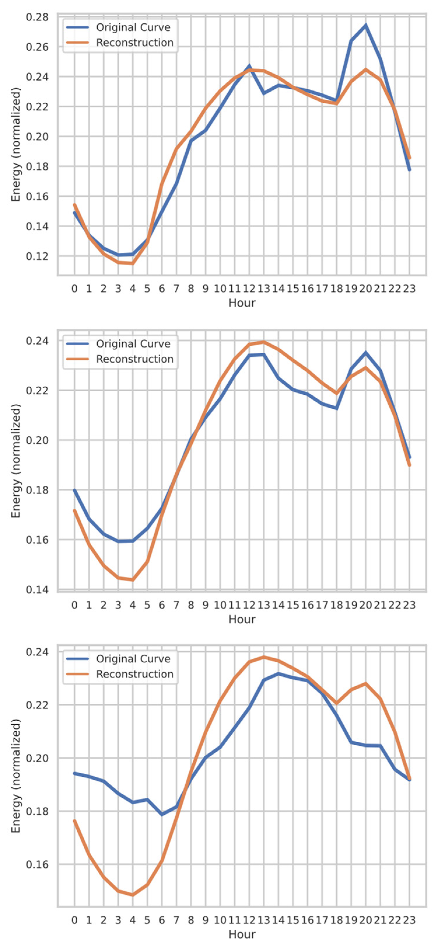
4.1. Operator A
This network operator delivered data from 16 substations, covering the period from 1 January 2020 to 30 June 2022. The substations are located in a temperate and mountainous area in central Colombia, and with this information, it was determined to work only with the eleven user clusters that exhibited an affinity with these geographical features. Most of these clusters show a relatively similar behavior, with low values between hours 0 and 5 for nearly all of them. The consumption peaks are more dispersed, with curves that rise in the afternoon or evening and others that are more stable throughout the day.
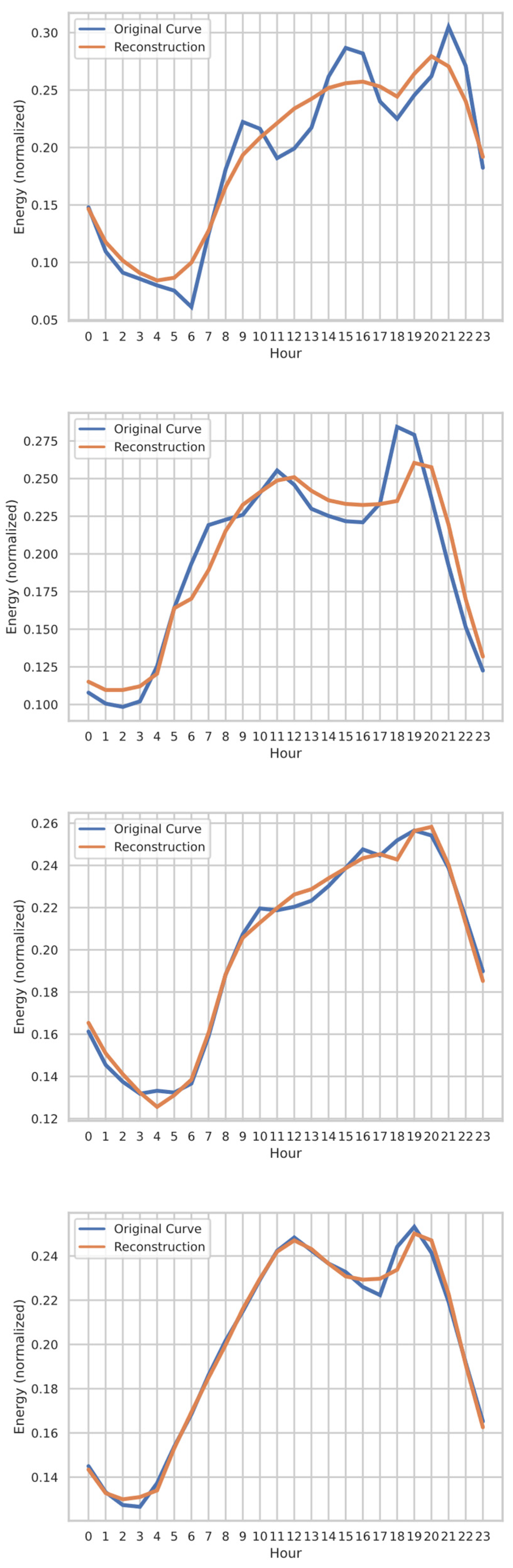
Figure 4 presents some examples of the curve approximations obtained using the model. The original curves of the substations are shown in blue, and the best reconstruction of each is shown in orange. The first two plots show significant dips in hours 0 to 5; the approximations are correct in both shape and magnitude, especially for the rise in the morning hours, although they are not quite correct regarding the minima and maxima. In the third plot, where the substation curve is flatter, the approximation is less accurate, failing noticeably in the early morning hours and slightly less in the evening hours.
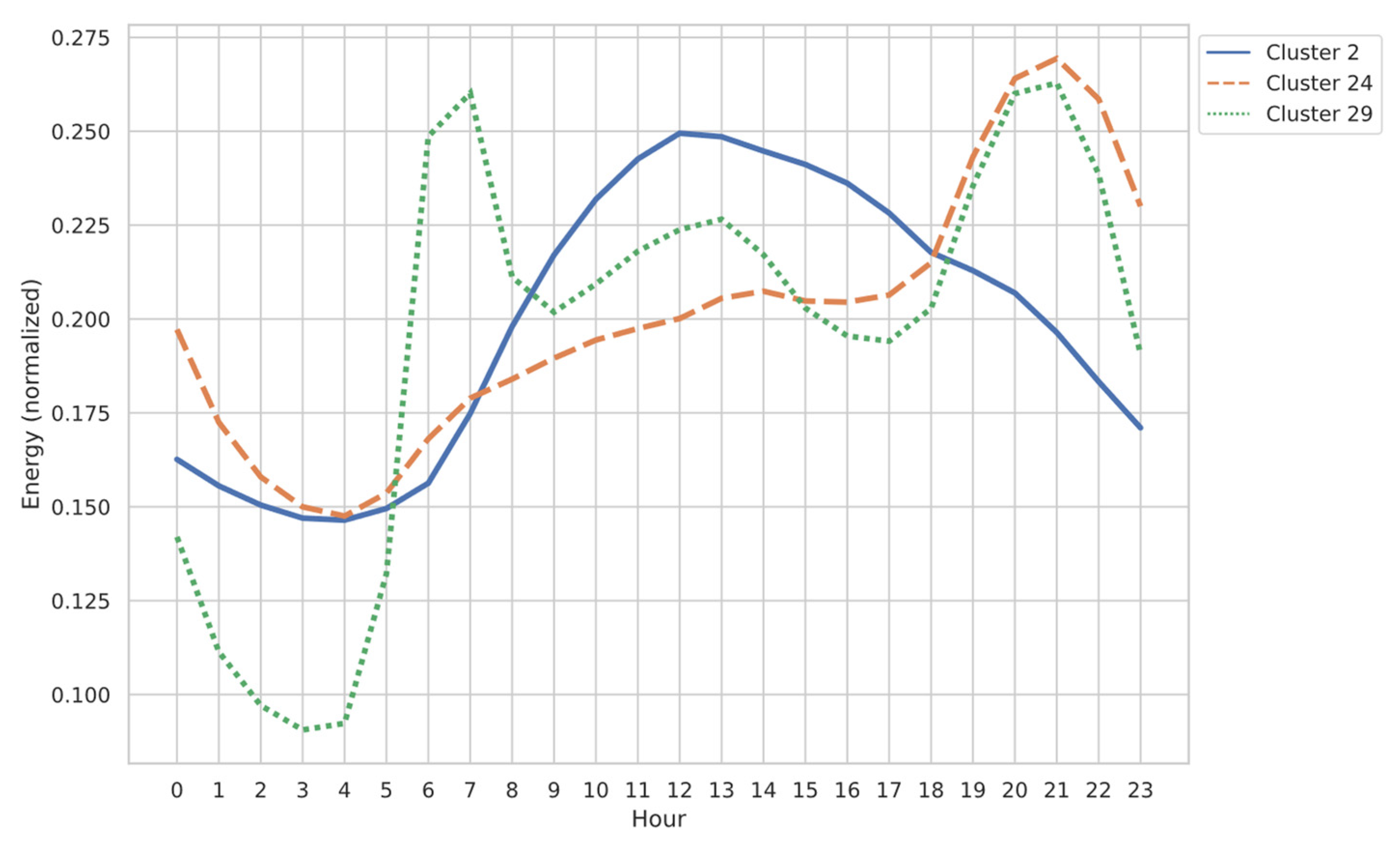
Regarding the weights of the clusters, the results show that in all cases, a significant portion of the weights have a value of zero, so the approximations can be described as the sum of only a few clusters, usually three or four. The most complex approximation depends on seven clusters. Also, some of the clusters tend to contribute to the reconstructions much more frequently than others, indicating that they could represent the vast majority of the behavior of the users in this geographic region. The three top clusters (whose weights are the largest in all the reconstructions of all the substations of this operator) are shown in
Figure 5, and they indicate that the most common load profiles for users show either valleys in the morning and peaks in the evening (orange and green curves, a residential behavior) or larger consumption in the afternoon than at night (blue curve, more commercial behavior).
In terms of the obtained characterizations, residential users are always given preeminence, and commercial and industrial users are in second and third place, respectively.
Table 2 presents a review of the most relevant statistics of the characterizations, where each column represents one of the user types. In no case does the model predict a proportion of industrial users greater than 1%, which is due to some bias in favor of residential users in the original clusters.
4.2. Operator B
This network operator delivered data from 19 substations covering the period from 1 January 2019 to 10 October 2022. The substations are located in a temperate region of Colombia. This unique restriction allowed for a larger number of clusters to be selected for the modeling. With a much larger number of clusters (27), there is a greater variety of geometries, and their curves exhibit peaks and valleys at multiple times of the day. However, most of the cluster curves show their lowest values between hours 2 and 7, and their highest values between hours 18 and 22.
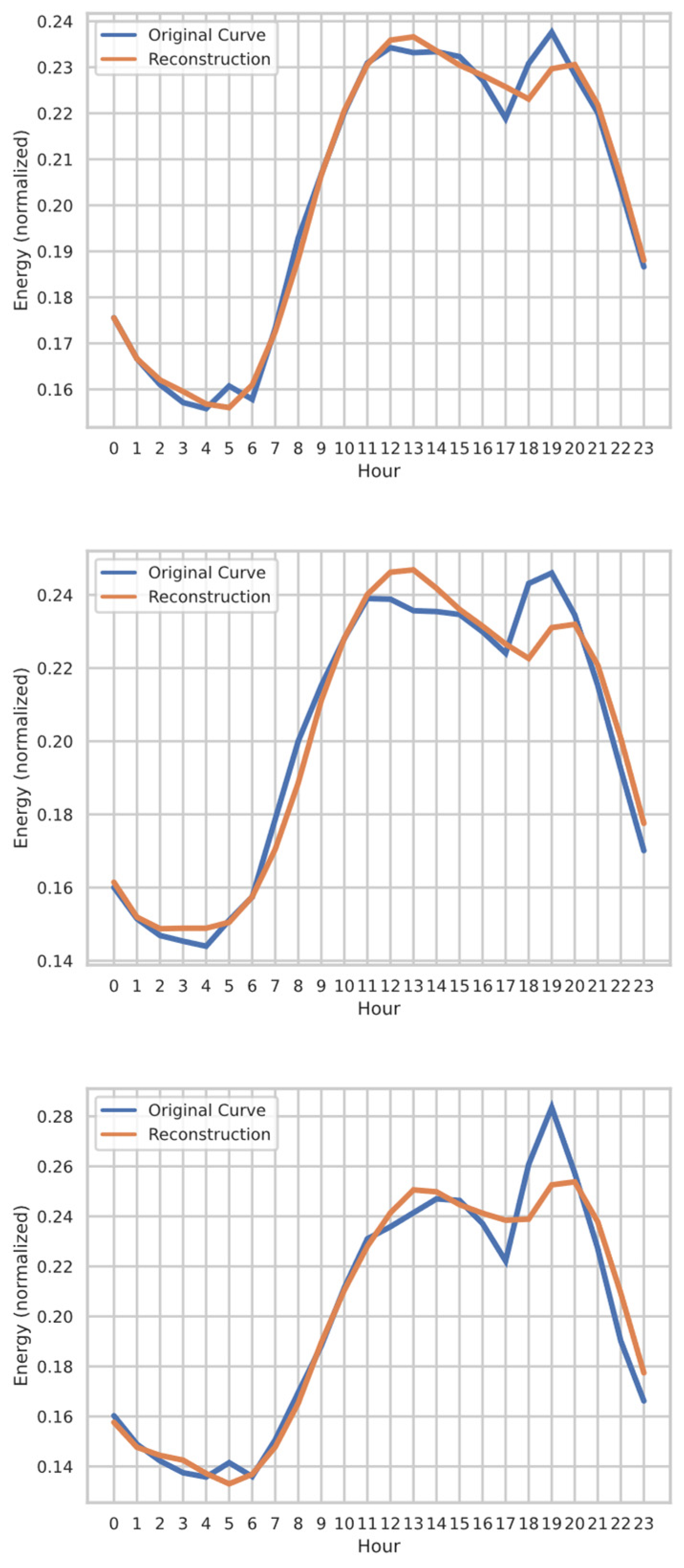
Figure 6 presents examples of the original curves and their reconstructions generated by the model. By having access to a greater variety of clusters, the approximations are much more accurate than those in the previous case. The model is able to capture, with remarkable accuracy, curves with different geometries (especially in the zones between hours 6 and 10 and at the end of the day), although again, there is a significant difference in the extreme zones (with the approximations being generally more moderate in their maximum and minimum points, with respect to the real curves). These discrepancies at the extremes are the most noticeable when these values correspond to steep, narrow valleys or peaks. In general, the model manages to capture the rise and fall moments correctly, making the geometries of the approximations quite accurate, except in the case of the most abrupt variations.
For this operator, the weights of the clusters are mainly concentrated in four areas. Six of the clusters always showed zero weights and therefore, were not part of any reconstruction. The clusters that concentrate the largest contributions in the reconstructions are shown in
Figure 7. According to these, the most common user profiles in the geographical region of Operator B include valleys in the mornings and peaks in the evenings (red curve, similar to the previous case, but with more variations throughout the day), or present the majority of the consumption in some specific range of hours and much less in others (noon and afternoon for the orange curve, afternoon and evening for the blue curve), or have a more consistent consumption throughout the day, with a slight increase in the early morning and a decrease in the evenings (as in the green curve). The red and green curves are more associated with residential users, and the blue and orange curves have more affinity with a commercial type of profile.
With regard to the characterizations, the dominance of residential users is a little less notorious than for the previous operator, varying between 89% and 96%, except in two particular cases, where it reached 83%; commercial and industrial users, always in second and third place, showed generally low proportions, but reached their highest values in the two aforementioned cases, reaching 14% and 3%, respectively. The complete statistics of the characterizations are presented in
Table 3, where it can be seen that commercial and industrial users obtain, on average, a slightly higher percentage than in the previous case. In addition, the dispersion of commercial and residential users remains similar in magnitude, and higher than that of industrial users.
4.3. Operator C—Database 1
This network operator delivered data from its substations covering the period from 1 July 2019 to 31 July 2022. The data were found in two different databases containing data from two different geographical areas, so a slightly different application of the model was performed for each. The smaller database (referred to here as Database 1) contained 14 substations located in warm areas of Western Colombia. Twenty clusters were selected for analysis using the data in Database 1, and their curves show multiple geometries: some curves exhibit peaks in the hours 0 to 4 and others in the hours 14 to 20; Some curves show low values all day, except for a few moments; and others are more stable throughout the day.
Figure 8 shows some examples of the obtained approximations. As in the previous sections, the model yields higher accuracy in the lower regions of the curves. Although in the higher regions, the curves may have a more noticeable separation, the model tries to mimic the geometry presented to it and manages to match the areas where the curve mainly rises or falls in the morning hours. In the afternoon hours, almost all the original substation curves exhibit high values between hours 10 and 22, which are separated by a somewhat abrupt drop at hour 17. Looking at the cluster plots, some of them show valleys around hour 18. Therefore, many of the reconstructed curves present a valley at hour 18, trying to approximate the dip in the original curves, but with a one-hour lag that results in differences between the originals and the reconstructions for hour 18 and later.
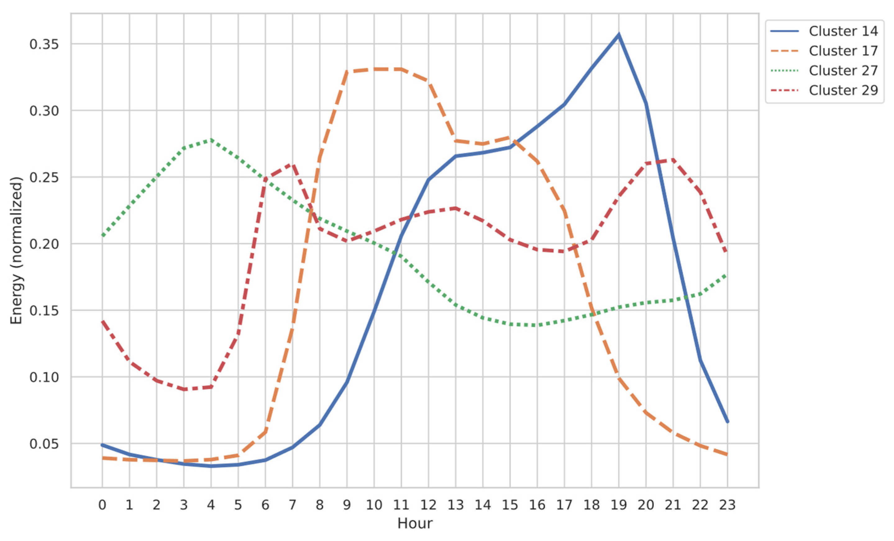
Regarding the weights of the clusters in the reconstructions, the model always assigned zero weights to half of the clusters, despite the variety of the geometries of the load curves. For the remaining ten clusters, the contributions are significantly concentrated in five of them, while the other five show lower weights and are not included in all of the reconstructions. The curves for the more important clusters are shown in
Figure 9, and they suggest that the behavior of the users in the areas around these substations often follows some patterns. They show a consumption that is much higher in the afternoon and evening, with decreases after midnight, either with a single peak around noon (green and orange curves) or with two distinct peaks (purple curve). Other behaviors include a consumption that increases steadily throughout the day and reaches its maximum in the late evening (red curve), or a consumption that decreases from the early morning until the evening (blue curve). Some of these clusters were also relevant in the previous sections, as two of them appear in the reconstructions for Operator A, and a third is mentioned for Operator B.
The characterizations were generally similar, with proportions of residential users ranging between 89% and 92%, and that of commercial users between 7% and 9%. There was a single record outside this trend, in which the proportion of commercial users rose to 14% of the total.
Table 4 shows the statistics of the characterizations, which present a much lower dispersion than did the previous statistics; in addition, the mean and median of the commercial and industrial users are much closer to the minimum, showing that the other characterizations are concentrated far from the anomalous case.
4.4. Operator C—Database 2
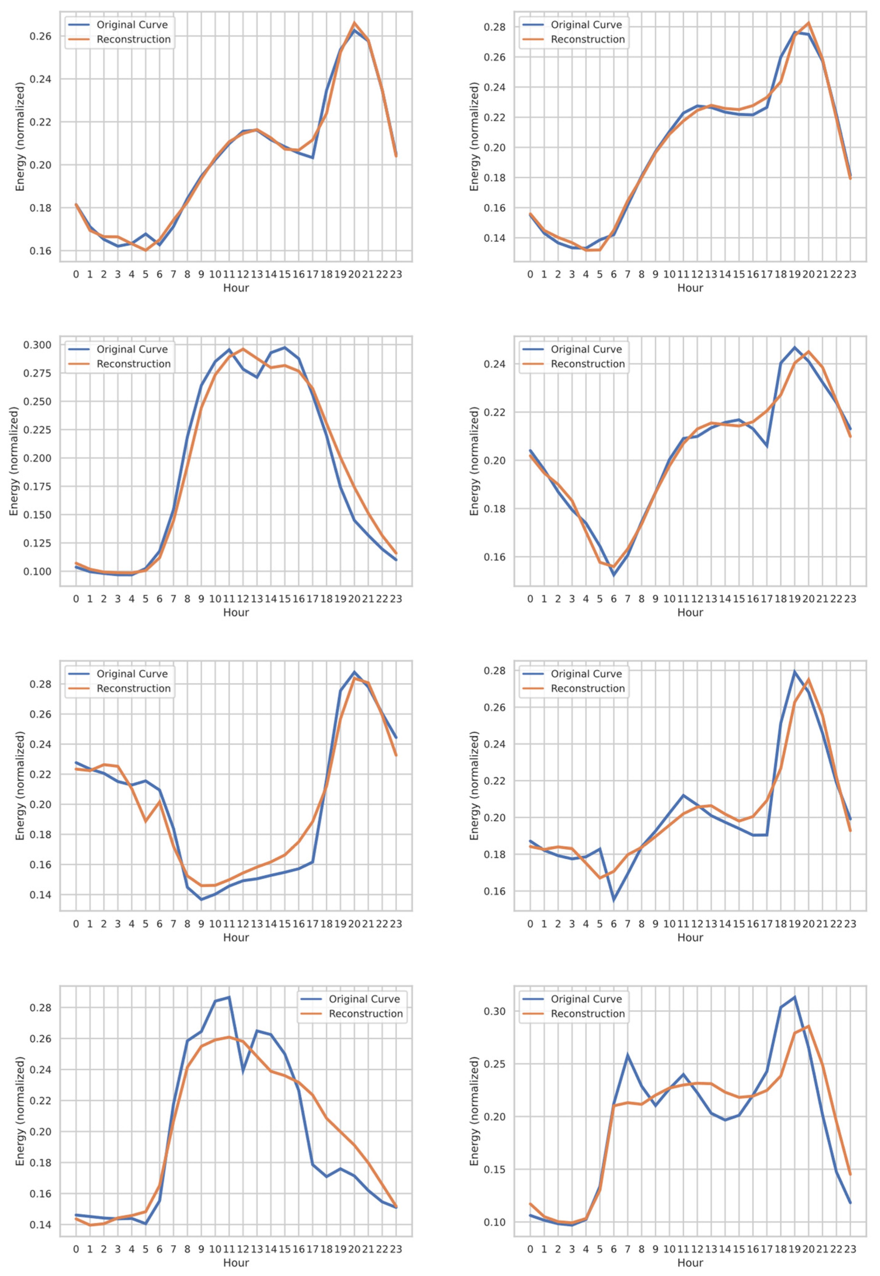
The second database of network operator C contains information from 345 different substations geographically distributed in Colombia, covering both warm and temperate environments, and both plains and mountainous areas. Since the geographical dispersion is greater in this case than in the previous examples, all the clusters could potentially be used; the twenty-five clusters with the most users were selected in order to include only the most representative ones. The curves associated with these clusters, similar to those in the previous case, show a remarkable variety of curve geometries, with curves showing peaks and valleys at different times. On average, most of the curves tend to have low values in the early morning (hours 1 to 5) and high values in the evening (hours 18 to 22), with a greater variety of behavior in the afternoon hours.
Similar to previous scenarios, the model approximates relatively smooth variations with high accuracy (especially the rise in consumption in the morning hours), but has difficulty with more pronounced variations, attempting to create curves where valleys and peaks are flatter. However, one strength of the model is that the curves it generates can exhibit various geometries, including the most common ones with low values in the early morning and high values in the evening, but also geometries with valleys in the afternoon or evening, or with high values in the afternoon falling off in the evening.
Figure 10 presents eight examples that represent the wide variety of substation geometries and how the model can approximate them with varying degrees of accuracy. The figure shows that the model yields its best approximations for smoothly varying curves, generally with early morning lows, afternoon plateaus, and evening peaks of varying magnitude. It can also handle distinct geometries, such as dips in the morning, a single peak in the afternoon, or a single peak in the evening. When more abrupt valleys or peaks appear, the model begins to show some differences, especially at the highest and lowest points, or in areas where the curve is more irregular. The most complex cases for the model are those with a succession of multiple peaks and valleys, as well as drastic rises and falls.
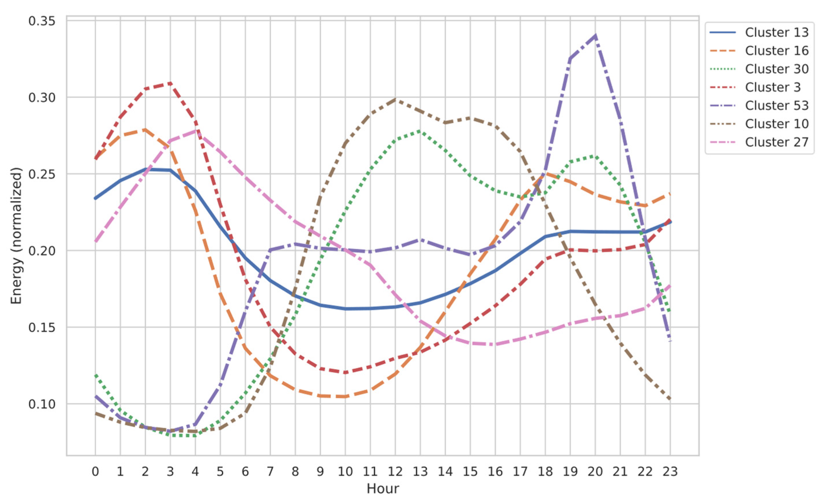
In contrast to all the previous cases, in which some of the clusters were completely discarded by the model by assigning null weights, all of them were used at least once, and none of them appear on all the reconstructions. However, some of the clusters appear much more frequently than others, and the curves of those that contribute in more than half of the reconstructions are presented in
Figure 11. The behaviors suggested by these clusters include some of the consumptions identified in the previous cases (such as the pink and brown curves), and the clusters can be easily distinguished in two groups, depending on how the curve behaves in the early morning. In the first group, we include the clusters with low consumption in the first hours of the day (green, brown, and purple curves), where consumption rises through the morning and decreases in late night, but whose peaks can appear at different hours of the day. The second group includes the clusters with higher values in the first hours of the day (blue, pink, orange, and red curves). The main difference between the curves of this group is the size of the variations, which can be noticeable (as in the red and orange curves) or small, resembling a flat line (blue curve).
In addition,
Table 5 presents the associated statistics of the characterizations obtained. With a much larger number of examples, the trend measurements show that most of the results point to high values for residential and low values for commercial and industrial users, although there is a non-negligible portion of substations that exhibit the opposite behavior, favoring the latter two types of users. The characterizations present a higher variation than in other cases (according to the dispersion values), thanks to the higher number of substations and their richer variety of curves.
5. Conclusions
This paper presents a methodology that encompasses the processing, analysis, and characterization of the substation data provided by three Colombian network operators, through the determination of appropriate features from each substation based on a series of load profiles built from groups of users. The core of such methodology is the formulation of the data reconstruction model, which uses a linear optimization model to approximate the substation curves from the curves of the clusters of users, and then uses the weights that define this approximation to determine the most common consumption behaviors of the users associated with the substation and also to estimate the proportions of three different types of users: residential, commercial, or industrial. The optimization model is also presented as a novelty with respect to processes currently implemented by the operators. In addition to the methodology, the results of its application on the data provided by the operators are shown. For each database, the preferred clusters for the reconstructions and some graphical examples of the application of the model are also presented.
The model is able to accurately approximate a wide variety of curves with different geometries and scales and obtained from areas, with different climates and geographical conditions. The best approximations are built using curves with relatively smooth changes and at magnitude values neither too high nor too low. In curves with many consecutive variations or with very deep peaks or valleys, the model fails to capture these, opting for a geometry that rises or falls, but in a softer form. This limitation may be due to the nature of the cluster curves, which were built as an average of hundreds or thousands of user curves. This masks the strongest variations that users would have had, and therefore, their geometries are smoother, making the reconstructions smooth as well.
For each operator and database, the clusters that appear in the majority of the reconstructions (and that contribute, to higher degree, to the approximations of the substations) are identified. The curves of these clusters can be seen as representations of the most common consumption patterns shown by users in each case. Although each case presents a different set of frequent clusters, some of them appear for multiple operators, allowing a broader identification of the consumption patterns of Colombian users. The load profiles include curves with various geometries that can grow or decline throughout the day, but that tend to yield their maximum values in the afternoon and evening. The identification of frequent load profiles can serve as a valuable tool in the middle-term planning of the electrical grid, since a better understanding of the electrical demand over a specific geographic region (such as average consumption, demand peaks, and other demand response-related issues) can help to determine the amount of electrical equipment required in each case. Therefore, this model could boost the success of future expansions of the grid in the areas of influence of the network operators, and it could also be applied in new areas where more network development is needed.
The characterizations in terms of user types always give preeminence to residential users, and commercial and industrial users are in second and third place, respectively, making up a relatively small portion of the users. The bias in favor of residential users can also be traced back to the construction of the clusters, in which this type of user accounted for a large majority of the data. Although the identification of users associated with the substation is a common practice by operators, it can be misleading because users exhibit many different behaviors, in addition to their labeled categories. These results, and the scheme that generates them, do allow for the individual analysis of user behavior in order to determine whether their categorization (residential, commercial, or industrial) agrees with the real consumption patterns, or whether it should be changed. This revision based on categories could be used to better understand general consumption patterns and to establish more fair tariff schemes in line with real consumption.
Although the results obtained are generally accurate, we have identified some limitations of our methodology when performing analysis on the consumption data. One of the most important requirements of our method is that the data must be taken on an hourly basis, but many AMI meters in the country are only set to take daily readings. Also, the data quality must be ensured beforehand, since the method either rejects null measurements or acts under the assumption that they can be replaced with average values. In the current state of Colombian AMI infrastructure, data quality is a major issue that can be affected by several external factors, thus impacting the validity of our results. Another relevant shortcoming of our proposed methodology is that it could not meet all the possible needs of the network operators in terms of data analysis, so a plausible line of research would be to couple the methodology with different methods of data mining and alternative analysis algorithms. These complements could potentially allow for the gathering of many other insights from the consumption data of both the users and substations.
A future line of work based on the results of this methodology may include the analysis of the variations in the curves under plausible scenarios of changes in electricity demand that could depend on specific types of users. These scenarios can include, among others, the massive installation of solar panels or other renewable energy sources or the charging of a large number of electric vehicles. Other lines of work may aim at selecting data mining techniques that can be coupled with the methodology in order to make it more robust, or to modify it to account the variations in consumption over the years. For example, the methodology could be modified to analyze in detail the influence that COVID-19 restrictions had on the electricity consumption patterns (and thus, the characterizations) of both the users and substations, since the data we used covered the period of the pandemic (as shown in
Figure 3). These results could then be extrapolated to future crisis scenarios that could occur in the country.
In summary, a demand characterization exercise based on AMI records is performed and used as a base to reconstruct the curves measured in the substations of the different network operators. This allows us to validate the existing relationships between user-level demand and aggregate demand in the nodes under study. Additionally, based on these results, it is possible to implement new ways of planning the distribution system and to verify how changes in the consumption by end users will affect the performance of the aggregate demand.


 ,
, 

