Abstract
The control systems for the variable-speed wind turbine based on the Doubly Fed Induction Generator (DFIG) pose some tuning challenges. The performance and stability of DFIG wind turbines during faults in power grids are directly related to their controller settings. This work investigates how incorporating protection via a braking-Chopper controller connected to the DC link (DC Chopper) and a reactive-current injection during the PI-tuning process affects the performance of DFIG wind turbines during electrical faults. For the tuning process, the Multi-Objective-Particle-Swarm-Optimization (MOPSO) algorithm was used. Thus, two different approaches adopting this methodology were investigated, considering sequential and simultaneous tuning. The results showed that sequential tuning presented a better performance in relation to the reactive-current injection and lower amplitude deviations of the electrical quantities during and after the fault. On the other hand, simultaneous tuning reached damping of the mechanical oscillations faster and presented better performance of the protection system.
1. Introduction
The variable-speed wind turbine based on the Doubly Fed Induction Generator (DFIG) is widely used today. The most common configuration consists of a horizontal-axis turbine, a turbine–generator mechanical coupling, a wound-rotor induction generator, and a back-to-back bidirectional power converter. The DFIG wind turbine is controlled by converters, and in most applications it uses Proportional–Integral (PI) controllers [1,2]. Topologies that use a braking Chopper in the Direct-Current-(DC) link also traditionally utilize a PI controller to regulate the DC voltage during faults in the electrical grid [3,4].
The control structures of these devices normally comprise current and active/reactive-power loops connected to the back-to-back converter as well as the DC-Chopper control [1,3]. Analyzing the operation of these control loops, it can be observed that the PI controllers of the back-to-back converter are active throughout all the operation scenarios (normal condition and fault events) of the DFIG wind turbine. On the other hand, the DC-Chopper controller only operates in the presence of electrical faults [5]. Thus, interactions between the control and protection may occur during faults, which depends on the intensity of the voltage sags. Therefore, it is imperative to consider these interactions in the tuning process.
The tuning of control system parameters plays a fundamental role in the performance and stability of the DFIG wind turbine. Due to the difficulties and complexity of tuning the DFIG wind turbine and the importance of the correct performance of control systems, several adjustment techniques have been proposed over the years, such as trial and error, linearization of the system (tuning through eigenvalues or using some specific algorithm) and classical techniques of control theory or optimization methods (ant-colony-optimization algorithm, genetic algorithm, etc.) [6,7,8,9]. Among the techniques tested over the years, one that has yielded good results is the Particle-Swarm-Optimization-(PSO) algorithm, which is recognized for being adaptable and capable of solving single- and multi-objective problems. In addition, this methodology enables optimization based on performance indicators (Objective Functions) extracted directly from dynamic simulations. This feature can quantify control behavior under electrical fault conditions and deal with all Objective Functions independently (multi-objective optimization) [2,6,10].
Hamid et al. [11] employed a novel Jaya-Particle-Swarm-Optimization-(JPSO) algorithm for the optimal tuning of wind-maximum-power-point tracking and DC-link-voltage PI-controller parameters. The results demonstrated a significant improvement in the steady-state and dynamic responses of DFIG controllers and a bidirectional energy-storage battery with DC–DC converter control connected to the DFIG’s DC link. Furthermore, the authors observed that by using the optimized PI controller gains tuning with JPSO: (i) the rotor speed converged more rapidly with precise reference tracking, leading to almost zero steady-state error, (ii) there was a reduction in the initial overshoot and a quick stabilization time during abrupt wind speed changes, (iii) the DC-link voltage exhibited a superior response with optimal tuning during load imbalances and abnormal grid voltage conditions. Jiang et al. [12] also used the PSO algorithm to solve the optimal reactive power demand of wind farms and to perform reactive-power allocation. Via simulations, they proved that DFIG operation without a unitary power factor can improve the system voltage quality and reduce grid loss, which is beneficial for a stable and efficient system operation.
Anilkumar et al. [13] applied the PSO algorithm, seeking to maximize the power exchange between the grid and the DFIG. It was observed that tuning with the PSO increased the overall energy savings in the system and minimized the use of capacitors. Kamel et al. [2] modeled a DFIG wind turbine with three PI controllers. Concerning tuning, they explored five optimization methods, aiming to improve the Low-Voltage-Ride-Through-(LVRT) performance. The study pointed out that the Hybrid Ant-Colony–Particle-Swarm Optimization was the technique that best adapted to the problem.
Regarding the system’s protection, Mosaad et al. [4] presented a new cost-effective technique to improve the performance of DFIG-based Wind Energy Conversion Systems (WECS) during wind gust and electrical faults, using high-temperature superconductors on the grids. They proved that the Fractional-Order-Proportional–Integral (FOPI) controller offers better results than a conventional PI controller. This is because it offers better control compared to the DC-Chopper duty cycle, improving the Fault-Ride-Through (FRT) capability during the events described. Pereira et al. [14] studied the influence between the crowbar protections on the rotor-side converter and the Chopper on the DC link. It was concluded that during a fault the DC Chopper allowed the DFIG to deliver reactive power, maintaining the voltage constant at the DC link and even preventing crowbar activation from minor faults. The DC Chopper also helped to meet the technical requirements of the Grid Code, mainly in terms of reactive-current injection. However, in the previously cited works, the interaction of the protection system and the DFIG’s operational system was not addressed.
Debre et al. [15] proposed a Chopper connected to the DC link, to control the imbalance in the stator and rotor currents and the fluctuation of the DC-link voltage during abnormal operating conditions. It was concluded that DFIG alone is unable to maintain the DC-link voltage during electrical faults, which can lead to equipment damage. On the other hand, the DC Chopper restricted the DC voltage rise, providing the necessary protection. Islam et al. [16] performed a transient analysis concerning the use of a DC Chopper to improve the Fault-Ride-Through (FRT) capability of the DFIG wind turbine. The authors also showed that the DC-Chopper resistor should be chosen carefully, especially because during an electrical fault a large value may affect the system’s performance. The work did not address the tuning process, nor the relationship between the electrical and mechanical quantities.
Thus, in order to understand the effects caused by DC-Chopper protection and reactive-current injection on the performance of a DFIG wind turbine during the tuning process of PI controllers, this work modeled parts of a DFIG wind turbine, its control system composed by PI controllers, the dynamics of the DC Chopper (which included a PI controller) and the reactive-current injection during electrical faults. For that purpose, two tuning methods using the Multi-Objective-PSO algorithm (MOPSO) were used, considering sequential and simultaneous tuning (referred to in this work as Method 1 and Method 2, respectively). It must be clarified that the MOPSO algorithm was responsible for determining the values of the gains of the PI controllers (with values between 0.0001 and 50), to achieve the tuning objectives.
Additionally, the DFIG wind turbine was tuned by the classical method called Symmetrical Optimum (SO) for comparative purposes.
This work adds contributions to the results presented in [6], especially concerning interactions with the protection system. This work builds upon the Ref. [6] study in the following aspects:
- It models the dynamics of the Grid-Side Converter (GSC). Ref. [6] did not model this part of the DFIG.
- It introduces protection and control systems during electrical faults (the DC Chopper). Ref. [6] did not consider any form of protection during faults.
- Due to more detailed modeling and the protection system, this work required tuning eight PI controllers, resulting in 16 gains to be defined. Ref. [6] tuned only five PI controllers.
- It considers reactive-power injection during faults. Ref. [6] did not consider reactive-power injection.
- Finally, this work aimed to understand the advantages and disadvantages of sequential and simultaneous tuning of the PI controllers with the MOPSO algorithm. Ref. [6] only investigated the possibility of tuning the DFIG with the MOPSO algorithm.
The main innovative aspects of this research are:
- Tuning the parameters of the DFIG’s PI controllers, using the multi-objective-PSO-(MOPSO) algorithm adapted to the wind turbine’s specific requirements;
- Considering the effects caused by the inclusion of protection and reactive-power injection during the tuning process of the wind-turbine control system;
- Formulating Objective Functions, to ensure that the DFIG complies with the Grid-Code requirements, which include supplying reactive power during an electrical fault.
2. Modeling DFIG Wind Turbines
This section presents the modeling of DFIG wind turbines, and therefore details the representation of a horizontal three-bladed turbine, a speed multiplier, an asynchronous generator, a back-to-back bidirectional power converter and the control and protection structure, including reactive-current injection during faults.
2.1. Wind-Turbine Modeling: Maximum-Power-Point Tracking
To model wind turbines, an algebraic approximation of the performance or power coefficient () model is used. The is a function of the pitch angle of the blades () and the specific rotation speed (), according to [1,6]:
where to are constants and depend on the construction characteristics of the turbine, R is the radius of the area swept by the blade, is the speed of rotation of the turbine and is the wind speed.
Thus, the mechanical power supplied by the turbine () has a fractional and non-linear relationship to the power contained in the wind flow (), and this fraction is given by the coefficient : . As explained in [17], when remains constant, the captured wind power varies if is modified. Thus, for greater energy efficiency, it is necessary to maintain the turbine operation at the point where is maximized. This strategy is known as Maximum-Power-Point Tracking (MPPT) and consists of maintaining with zero value and adjusting the angular turbine velocity () according to the wind-speed variation [17], which results in the power curve illustrated in Figure 1.
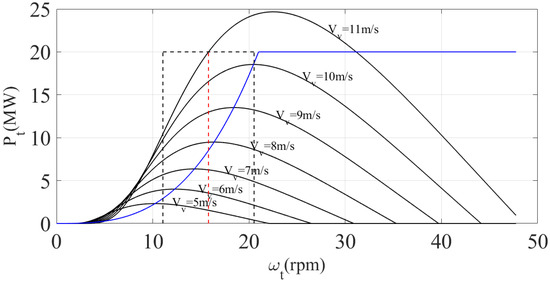
Figure 1.
Maximum-Power-Point-Tracking (MPPT) strategy. Black-dashed-line: range of speed variation of the turbine. Red dashed line: synchronous speed. Blue line: power (Maximum-Power-Point-Tracking strategy).
In Figure 1, the black-dashed-line rectangle indicates the range of speed variation of the turbine around the synchronous speed (the red dashed line). In this range, the turbine can operate with power, according to the blue line (the Maximum-Power-Point-Tracking strategy).
The mechanical coupling is represented by the two-mass model, whose equations can be found in [6]. The wound-rotor-induction-machine model is also taken from [6], which is given in coordinates in the synchronously rotating reference frame, with magnetic fluxes as state variables, and all variables and parameters are expressed in p.u.
2.2. Current and Power Control Loop
A back-to-back power converter is used to allow the power flow between the DFIG rotor and the grid. It consists of two inverters, one on the rotor side and the other on the grid side, which share a DC link. This work used the “Vector Control Oriented by Stator Voltage” method [1,6,18].
Figure 2a shows the rotor current and the active- and reactive-power control loops. The total active power is controlled by acting on the direct-axis component of the rotor current . For stator reactive power (), the control is performed by acting on the quadrature-axis component [19].
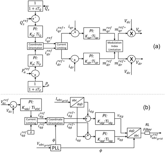
Figure 2.
Control systems for RSC, GSC and DC link. (a) RSC’s control systems. (b) DC link and GSC’s control systems.
In Figure 2a, the time constants and represent the dynamics of the filters for the active- and reactive-power measurements. The reference signal for the total active power generated by the DFIG wind turbine is given by the difference between the active power calculated by the MPPT strategy and the electrical losses of the DFIG’s stator and rotor. Figure 2a shows four PI controllers and, consequently, eight parameters to be tuned, because each PI has a proportional gain (K) and an integral time constant ().
The DC-link voltage () is controlled by a PI controller, and the control-loop structure is shown in Figure 2b. The PI controller receives the DC-voltage error signal and determines the signal and reference of the direct-axis-current control loop of the GSC, acting on the reference of the direct-axis current of the GSC () [1,20].
In the GSC control, the quadrature axis reference () is typically set to zero, to ensure the operation of the converter with a unit power factor [1]. Moreover, a current limiter is used, to prevent the excessive increase of .
The GSC-current control loops (see Figure 2b) receive the reference values and resulting from the DC-link control loop, the current limiting and the coordinates’ orientation according to the angle determined by the Phase-Locked Loop (PLL), and then compare them to and , respectively. Then, the error signals are processed by the PI regulators, which provide the voltages and [20].
The sinusoidal three-phase voltage at the GSC output is determined by transforming the voltage values from the reference to the , based on the angle determined by the PLL. The desired voltage () is sent to the Pulse-Width-Modulation-(PWM) converter, to be applied to the electrical grid [20]. Thus, Figure 2b shows three more PI controllers, therefore, six more parameters to be tuned.
The control structure considered in this work incorporates additional reactive-power control mechanisms addressing the requirements of current Grid Codes (GCs) on the DFIG wind turbine’s capacity to inject/absorb a reactive current during faults. Although the methods used here can be adapted to other GCs, this work refers specifically to the Brazilian case [21].
According to the Brazilian Grid Code (see Figure 3), a wind farm must be able to inject a reactive current during voltage dips in which the grid voltage drops below 0.85 p.u. and needs to be able to absorb a reactive current while the grid voltage is higher than 1.1 p.u.
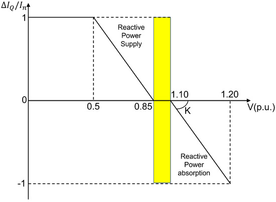
Figure 3.
Brazilian Grid Code with reactive-current requirements. Yellow area: reactive-current reference is zero [21].
Figure 3 shows a yellow area where the reactive-current reference is zero. When the voltage leaves the yellow area, having a value above 1.1 p.u. or less than 0.85 p.u., the DFIG wind turbine must absorb or supply, respectively, a reactive current to the grid.
The control strategy for reactive-current injection/absorption adopted in this work was derived from [22] and is based on modifying the reactive-power control reference during the fault and according to the grid voltage level (). Considering the requirements of the Grid Code as shown in Figure 3, the reactive-current () injection and absorption are as described below:
As the control structure requires a reactive-power reference, Equations (3) and (4) can be used to build up the reactive-power reference () according to the voltage level, in the form of
All control loops use conventional PI controllers, each one with the usual tuning parameters: a proportional gain (K) and an integral time (). Therefore, aiming at the stability and correct operation of the wind farm, the values of all parameters K and must be determined. In addition, when an electrical fault occurs, the DFIG protection system is triggered, which will be explained in the following subsection.
2.3. DC-Chopper Protection System for DFIG Wind Turbines
When an electrical fault occurs in the system and the voltage dip is not severe, the system can be controlled by converters. However, when the amplitude of the voltage dip is considerable, the currents and voltages of the converter cannot be limited by the control system alone. In order to deal with this, there are some protection schemes that prevent damage to the converter by overcurrents and overvoltages of the DC link [3]. The protection system is called Chopper and consists of a bank of resistors that acts by dissipating power during the fault, as part of the current is diverted to the resistors, producing an efficient reduction of the current or voltage levels [3].
The protection used in this work was a DC Chopper that consisted of a resistance controlled by transistors. The resistor could be connected or disconnected using a switch (transistor), as shown in Figure 4a. This strategy was used to limit the excessive voltage on the DC link, and it consisted of the most advanced solution today among those that do not rely on storage systems [5]. When adding a resistance controlled by a transistor to the DC link, there is no need to disconnect the converter during faults, as this device helps to prevent an excessive increase in the DC voltage. As a consequence, the wind turbine can be controlled during electrical faults [5].
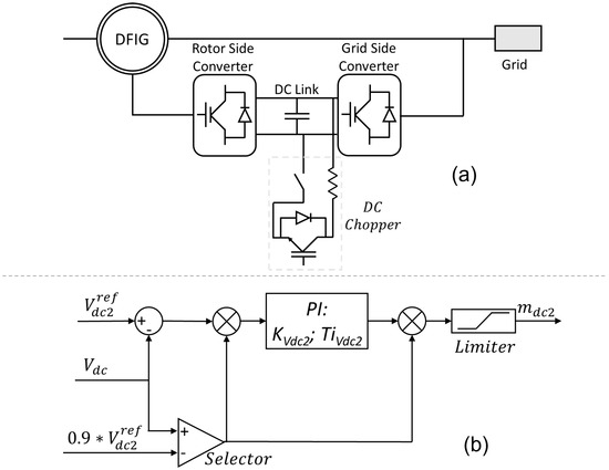
Figure 4.
DC Chopper connection and control schemes. (a) Resistor could be connected or disconnected using a switch (transistor). (b) DC Chopper control system.
Due to the Chopper operation type, a control is needed for its activation and disconnection. The control used in this work is shown in Figure 4b. In order to respect the overvoltage limits of the converter, the Chopper control uses a voltage reference greater than the nominal . The Chopper operates only when the DC bus voltage exceeds 90% of the reference voltage value, and in Figure 4b this action is shown, using the “Selector”, in which if is less than 90% of the output is zero and if is greater than 90% of the output is one. Finally, the output of the PI controller goes through a limiter, and is used to perform the PWM modulation of the Chopper switch [3,5].
Figure 2 and Figure 4 show a total of 16 PI gains to be tuned. However, the Chopper PI is only activated when severe faults occur. Before performing the tuning process, qualitative and quantitative criteria need to be established, to measure the performance of the wind farm, which will be explained in the following section.
3. Main Tuning Objectives Considering an Electrical Fault
Considering the growth of wind generation, the LVRT capability for wind turbines is a requirement of the GC in almost all countries that have this type of generation [2]. For the correct operation of the DFIG wind turbine, some internal operational requirements need to be met. For this reason, in this section, the performance and damping criteria for tuning the PI controllers of the DFIG wind turbine are established. These criteria are:
- Grid-Code Compliance—Voltage (V): the voltage should remain in the gray region, shown in Figure 5, during the fault and present a post-fault recovery without major peaks.
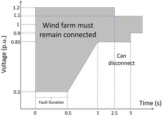 Figure 5. Brazilian Grid Code with voltage requirements [21].
 - Damping of mechanical oscillations: rotor and turbine speeds must converge to the same value and must show damped oscillations [6].
- DC-link voltage with low variation: To ensure safety during and after an electrical fault, = 1.2 p.u. is established as the maximum limit [3].
- Low-peak currents: to avoid overcurrents, the maximum permitted values are: bus current, 3.5 p.u.; converter current, 1.5 p.u.; rotor and stator current, 3.5 p.u. [1] (p. 96).
- Decrease in peaks and fluctuations in active power P: to facilitate recomposition after an electrical fault, maximum active power = 2 p.u. [6] is established.
To achieve these objectives, the MOPSO algorithm uses the following equations:
where = simulation time, = variation of the torsion angle that measures the difference between the turbine and the generator rotation speeds, i = bus current, Q = reactive power, = DC link voltage, = total active power and = reference value.
All Objective Functions were penalized by IAE (Integral Absolute Error), which was an natural choice for this research, as it was necessary to measure dynamic errors and to penalize them according to the magnitude of the deviation, giving equal weight to deviations that occurred at the beginning and at the end of the simulation [23,24].
4. Operating Conditions and Tuning Methods
The system used for testing the proposed tuning algorithms was a wind farm comprising 10 DFIG wind turbines connected to an infinite-bus system (see Figure 6. The infinite-bus voltage was 1.0 p.u. the short-circuit capacity seen from the connection point was = 4 p.u. and there was a transmission line with ratio X/R = 8. The parameters of the DFIG wind turbines are shown in Table 1, and two tuning methods using the Multi-Objective-PSO algorithm (MOPSO) were used, considering sequential (Method 1) and simultaneous (Method 2) tuning.
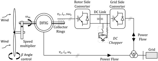
Figure 6.
DFIG wind turbines used for tests.

Table 1.
DFIG wind-turbine parameters used for tuning and testing.
In Method 1, the PI controllers were tuned sequentially, starting by the parameters of the PI controllers of the active and reactive power, the DC-link voltage and the rotor- and converter-current control loops. Then, the PI controller of the DC-Chopper control loop was tuned. For the first phase of Method 1, a low-intensity electrical fault was simulated, so as not to cause the protection to trip, which was a fault with a voltage dip up to 0.7 p.u. and a duration of 500 ms (the maximum allowed by [21]). Then, having already tuned the PI-controller parameters of the converter, a more severe fault was simulated (voltage dip up to 0.3 p.u. with a duration of 500 ms), which caused the trip of the DC-Chopper protection, making it possible to tune the PI-controller parameter of the DC-Chopper protection (see Figure 4b).
In Method 2, all the PI controllers were tuned together. To do this, the occurrence of a fault that would cause a voltage dip up to 0.3p.u. with a duration of 500 ms was simulated. This fault caused the trip of the DC-Chopper protection, making it possible to tune all the PI controllers in the DFIG wind-turbine control structure simultaneously.
In order to compare the performance of the DFIG wind turbine obtained with the PSO tuning, the DFIG wind-turbine controllers were also tuned with the Symmetrical-Optimum method, a procedure that only takes into account decoupled-transfer-function approximations of the control loops.
Using the previous parameters and the requirements established in Section 3, two methods were established to tune the PI parameters with the Multi-Objective-PSO algorithm.
5. Multi-Objective-Particle-Swarm-Optimization Algorithm Used for Tuning
Particle-Swarm Optimization (PSO) is a heuristic search technique with a population of solutions, where each individual of the population is a possible solution to the problem. Due to its simplicity and its ability to solve non-linear, continuous and multi-objective problems, it is ideal for optimizing DFIG wind-turbine control systems [2,6].
The MOPSO algorithm proposed in this work extends the one used in [6] in the following aspects: (i) in order to comply with the two tuning methods, MOPSO was applied sequentially and under different test conditions; (ii) the decision maker was adapted to each of the two faults required by the tuning process and the “solution region”, as each voltage dip had to be modified; (iii) due to the coupling of the DFIG wind turbine variables, it was possible to decrease the set of Objective Functions; thus, the bus current was the only current penalized in the Objective Functions; (iv) due to the inclusion of the reactive-current injection, the representation of the controls associated with the GSC and the DC-Chopper protection, there was an increase in the number of parameters to be tuned.
Therefore, this research presented eight PI controllers resulting in 16 variables to be tuned.
The step-by-step procedure of the MOPSO algorithm is shown in Algorithm 1. The “Initial phase” assigned a position between [] and a random velocity between [] to each particle (Step 1).
In Step 2, to meet the tuning requirements of Section 3, a set of six Objective Functions was established, Equations (9) to (14).
After calculating the Objective Functions (OFs) in Step 2, the best position was defined for each particle so far, the pbest (Step 3), copying the value of the dimensions of its corresponding individual. In Step 4, the Pareto Front was defined [6].
In the last step of the “Initial Phase”, the Decision Maker determined the “solution region” (Step 5), defining the maximum value that each Objective Function could reach. As explained in [6], for the setting of the “solution region” a value was established for each Objective Function, such that for a particle to be in the solution region all Objective Functions had to attain values less than or equal to the respective . As the “solution region” depended on the operating and testing conditions, two solution regions needed to be built: the first was valid for a voltage dip up to 0.7 p.u. and the second was valid in the case of a voltage dip up to 0.3 p.u.
The Decision Maker determined the following particles when updating the velocity vel (see Equation (15)). Thus, three situations could happen: (i) no particle reached the “solution region”, therefore, the lbest leaders were the particles that were in the Pareto Front; (ii) a particle reached the “solution region” and it was in the Pareto Front, therefore, all particles used it to update their velocity; (iii) two or more particles reached the “solution region” and the Pareto Front, establishing themselves as the leaders of the algorithm, and the other particles used them to update their velocity. In case (iii), the choice of which particle to follow was random and did not change unless some other particle reached the “solution region” and the Pareto front.
The second stage, MOPSO’s “search phase”, was where the iterative process took place. Thus, for each particle the Objective Functions were calculated (Step 6) and analyzed for the possible improvement of pbest, with two possible situations: (i) if all the Objective Functions attained values smaller than or equal to (none greater than) the respective values for pbest, then the pbest and the Pareto Front were updated (Step 7), and then it proceeded to the Decision Maker (Step 8); (ii) if pbest had not been improved, it passed directly through the Decision Maker (it went to Step 8 without going through Step 7). In Step 9, the velocity vel of the i particle was updated in the j dimension, and then the x positions were updated with the Equation (16):
where and are cognitive and social learning factors, respectively, and are randomly generated numbers with uniform distribution in the interval [], is the inertia factor and is the iteration number.
In Step 10, it was checked if any particle had crossed the search space and, if so, it was brought to the border and its velocity was reset. In the case that the termination criterion was not met—that is, the maximum number of iterations () was not reached—the iterative process continued, returning to Step 6. In the case that it was reached, it finally passed through the decision maker, to establish the gbest algorithm solution (Step 11). In this case, gbest was the particle found in the “solution region” and in the Pareto Front with the lowest cost of (the particle that damped the mechanical oscillations more quickly).
| Algorithm 1: Step-by-step procedure for the MOPSO algorithm. |
Initial phase: 1. For each dimension of each particle: random position between [ and ] and random velocity between [ and ]. 2. Calculate set of Objective Functions. 3. Define the best place for each pbest particle. 4. Define Pareto Front. 5. Decision maker: determine “solution region”. Search phase (iterative process): 6. Calculate set of Objective Functions. Is the new pbest better?? Yes → go to Step 7. No → go to Step 8. 7. Update pbest and Pareto Front. 8. Decision maker: determine particle to follow in the velocity update. 9. Update velocity and positions. 10. Check positions. Termination criterion? Yes → go to Step 11. No → go to Step 6. 11. Decision maker: determine gbest solution. |
6. Tuning Methods and Tuned Control Parameters
In the following subsections, different values of the PI parameters obtained with the MOPSO algorithm will be presented, as well as the classic Symmetrical-Optimum method used for comparison. For tuning with MOPSO, the following parameters were used for the algorithm: particle population, 100; search space, = 0.0001, = 50; limiting velocities, = −5, = 5; cognitive factor, = 2; social factor, = 2; inertia, w, which decreased linearly with the number of iterations, from 0.9 to 0.4; and , numbers generated randomly at each iteration and evenly distributed over the interval = 0 and = 1; maximum number of iterations = 100 (termination criterion) [6].
6.1. Method 1: MOPSO Applied to Tune the PI Controllers Sequentially
For Method 1, initially, it was necessary that the fault did not cause protection trips. Thus, using the MOPSO algorithm with a fault that led to a decrease in voltage up to 0.7 p.u. and with the shown in Table 2, the values of the PI parameters of the control structure of the DFIG wind turbine were obtained, except for the DC-Chopper-PI controller ( and ). Thus, in this first execution of the MOPSO algorithm, the values of the Objective Functions shown in Table 2 were reached.
Table 2.
Objective Function values (without unit) with voltage dip of 0.7 p.u. for Method 1.
In the second step of Method 1, only the tuning of the DC-Chopper-PI parameters was performed. To do this, the parameters of the already-tuned PI controllers were fixed and the second fault was applied, leading to a voltage dip of 0.3 p.u. and the tripping of the DC-Chopper protection. Then, the MOPSO algorithm optimized only the loop (see Figure 4), determining the values of and . The used and the values of the Objective Functions achieved in this second execution of the MOPSO algorithm are shown in Table 3.
Table 3.
Objective Function values (without unit) with voltage dip of 0.3 p.u. for Method 1.
Thus, for Method 1, the values of the PI-controller parameters summarized in Table 4 were obtained.
Table 4.
PI-controller parameters obtained with MOPSO, Method 1.
6.2. Method 2: MOPSO Applied to Tune All PI Controllers Simultaneously
For Method 2, the 16 parameters of the PI controllers were tuned simultaneously. For this purpose, a fault that dropped the voltage to 0.3 p.u. was simulated, a condition in which the DC-Chopper protection tripped, allowing and to be tuned together with the converter-controller parameters.
Thus, the Multi-Objective-PSO algorithm with the (shown in Table 5) was executed and the Objective Function values summarized in Table 5 were obtained.
Table 5.
Objective Function values (without unit) with voltage dip to 0.3 p.u. for Method 2.
Finally, the obtained tuned values of the PI parameters for Method 2 are presented in Table 6.
Table 6.
PI-controller parameters obtained with MOPSO, Method 2.
It should be noted that internal control loops and are analogous, similarly to loops and . However, the parameter values tuned with the MOPSO algorithm (for both Methods 1 and 2) for these loops were not the same.
6.3. Tuning with the Symmetrical-Optimum-(SO) Method
The SO is a classic method that tunes controllers from the knowledge of the control loops reduced to their linear and single variable representations [25].
In [6], the SO method was also used to tune the PI controllers of the DFIG wind turbine. However, in the current work, the GSC and DC-Chopper-protection control loops were added, having a more detailed modeling, making it necessary to take into account the relationship between the internal loop of the GSC and the DC link. References [6,25] present more details on the step-by-step application of this method.
The values of the PI parameters with the SO method are presented in Table 7. It should be noted that the tuning process with the SO method does not depend on the operation point, transient disturbance, non-linearities or couplings between the DFIG-wind-turbine control loops.
Table 7.
PI-controller parameters obtained with SO.
7. Performance of the DFIG Wind Turbine
This section presents the simulation results concerning the performance of the DFIG wind turbine with the parameter tuning of the PI controllers developed in Section 6. Two tuning methods with the Multi-Objective-PSO algorithm were proposed, and the MOPSO-1 (Table 4) and MOPSO-2 (Table 6) abbreviations were used here to refer to the PI controller parameters obtained by Methods 1 and 2, respectively. Simulations were performed for the system, considering electrical faults with two different levels of voltage drop. In order to detail the performance of the DFIG wind turbine, the results for the mechanical and electrical variables are presented with different timescales (30 s and 3 s), respectively.
The first test considered an electrical fault that did not trip the DC-Chopper protection. To do this, the same electrical fault used in the first step of Method 1 (see Section 6.1) was chosen, with a voltage dip of 0.7 p.u.
Figure 7 shows the behavior of the mechanical variables of the DFIG wind turbine for the first test. Comparing the behavior of the mechanical variables of the DFIG wind turbine for the different tunings, it was noticed that the tunings provided by the MOPSO algorithms were the only ones able to dampen the rotor and turbine speed oscillations.
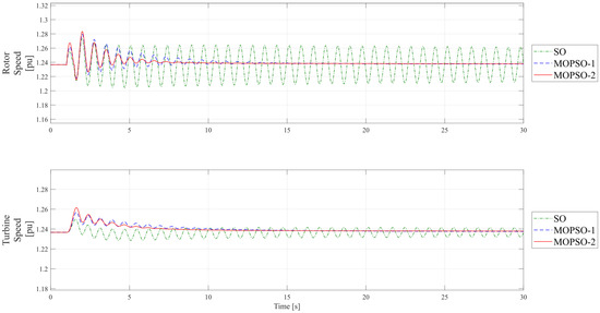
Figure 7.
Comparison of DFIG-wind-turbine performance with voltage dip of 0.7 p.u. mechanical variables.
This is one of the main advantages of the proposed Multi-Objective-PSO algorithm. Favoring the damping of the mechanical oscillations of the DFIG wind turbine under the tested conditions was a difficult control objective to be achieved. As a matter of fact, the tuning with the SO method was not able to achieve this goal (the rotor and turbine speeds did not converge to the same value after the fault period). Thus, the tunings with MOPSO were the only ones that met the damping requirement of Section 3. Moreover, the MOPSO-2 tuning was able to dampen the oscillations faster than the MOPSO-1 tuning, a behavior attributed to the simultaneous tuning of the PI controllers.
Figure 8 shows the behavior of the electrical variables of the DFIG wind turbine for the first test. As expected, the DC-Chopper protection did not trip during the first test (“Chopper Activation = 0 ”) and, therefore, there was no power dissipation by the protection (“Protection Power = 0”). The terminal voltage V, in all tunings, remained within the LVRT region determined by the Grid Code (GC: ) (see Figure 5). The voltage level during the fault was similar for both the MOPSO-1 and the MOPSO-2 tunings (slightly higher for the MOPSO-1 tuning), with damped oscillations and a post-fault recovery without large overvoltage peaks. Thus, the MOPSO-1 and MOPSO-2 tunings met the voltage requirement established in Section 3, improving the LVRT capability of the DFIG wind turbine.
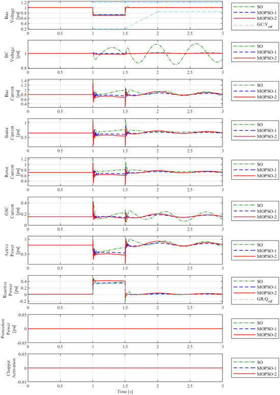
Figure 8.
Comparison of DFIG0-wind-turbine performance with voltage dip of 0.7 p.u. electrical variables.
Both the MOPSO-1 and the MOPSO-2 tunings resulted in small variations and damped oscillations of the DC-link voltage, ensuring the safety of the DC link during the fault (see Section 3). In addition, the MOPSO-2 tuning showed faster dampening of the oscillations than the MOPSO-1 tuning both during and after the fault.
Regarding the behavior of the currents with the MOPSO-1 and MOPSO-2 tunings, the peaks reached were below the maximum allowed ( p.u; p.u; p.u; p.u), preventing equipment problems and disconnection due to overcurrents. Comparatively, the MOPSO-2 tuning showed higher maxima and more damped oscillations than the MOPSO-1 tuning during the fault. On the other hand, MOPSO-1 showed higher peaks at the end of the fault. In the post-fault period, the currents presented more dampened oscillations with MOPSO-2 tuning, but with greater amplitude if compared to MOPSO-1.
The active power dropped during the fault, attaining the lowest level for the MOPSO-2 tuning, which, nonetheless, showed more dampened oscillations than MOPSO-1, both during and after the fault. In addition, the MOPSO-2 tuning had a lower minimum and a greater amplitude of oscillations after the fault. The highest peaks appeared when the fault was cleared, but without exceeding the pre-set limit ( = 2 p.u.; see Section 3) for both MOPSO tunings. However, the P maximum for the MOPSO-1 tuning was greater than the maximum for MOPSO-2.
One of the most significant differences between the tunings with MOPSO was the error regarding reactive-power injection. The MOPSO-1 tuning achieved better tracking of the Q reference (GC: , given by Equations (5) to (8)), with more dampened oscillations and smaller amplitude peaks than the MOPSO-2 tuning. Thus, the MOPSO-1 tuning helped the wind farm to comply with the Grid Code, and the DFIG wind turbine operating with the tuning obtained from the MOPSO helped support the voltage during faults, providing the reactive power requested by the GC. The MOPSO-2 tuning was less effective, as it delivered a higher Q value during the fault while showing a lower voltage level.
On the other hand, due to the unstable behavior, the DFIG-wind-turbine performance with the SO was not able to meet the requirements established in Section 3. This was because the tuning with the SO showed undamped behavior of the mechanical variables, a strong peak in the terminal voltage at the time the fault was cleared, strong fluctuations in the DC link voltage, high amplitude peaks in currents and deficient convergence of reactive-power Q to the reference value (especially after clearing the fault from the system). The DFIG wind turbine, operating with the tuning obtained from the SO method, was disconnected, due to instabilities.
The results of the first test showed the good performance of the DFIG-wind-turbine electrical and mechanical variables obtained with the MOPSO tuning algorithms. In general, with MOPSO-2 tuning, faster damping of mechanical and electrical oscillations was achieved, both before and after the fault. However, the MOPSO-1 tuning showed better tracking of the reactive-power injection reference, also resulting in smaller voltages and active power drops during the fault.
The second test considered a more severe electrical fault causing a terminal voltage dip of 0.3 p.u. This was the second tuning step in Method 1 and the tuning condition in Method 2 (see Section 6.1 and Section 6.2, respectively). In this case, the dynamic behaviors of the mechanical and electrical variables are shown in Figure 9 and Figure 10, respectively.
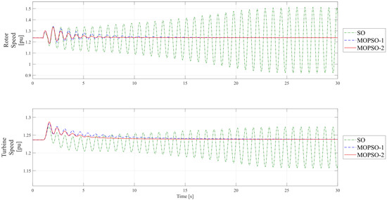
Figure 9.
Comparison of DFIG-wind-turbine performance to voltage dip of 0.3 p.u. (mechanical variables).
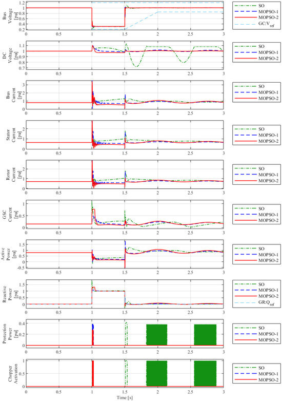
Figure 10.
Comparison of DFIG-wind-turbine performance with voltage dip of 0.3 p.u. electrical variables.
The major differences between the tunings with the MOPSO algorithms and the SO method were found in the mechanical part (see Figure 9). Again, only the tunings with the MOPSO algorithms were able to dampen the mechanical-variable oscillations and reach the convergence of both rotor and turbine speeds. Moreover, similar to the result of the first test, the MOPSO-2 tuning was slightly more efficient in damping the oscillations in the turbine and generator speeds. The faster damping of oscillations provided by the MOPSO-2 tuning can be observed in Figure 9, and a comparison of the values of Cost (which measured the damping of the mechanical oscillations) in Table 3 and Table 5 further supports this observation. For Method 1, Cost = 74.1136, while for Method 2, Cost = 39.8496.
Once more, tuning with the SO method did not meet the requirements established in Section 3.
The “Chopper Activation” variable (see Figure 10) shows the protection trip during and after the fault. With the MOPSO-1 and MOPSO-2 tuning, the DC Chopper was only triggered during the fault period and for a short period of time. Moreover, due to the simultaneous tuning of all the PI parameters, the MOPSO-2 tuning performed better, dissipating less power via the DC Chopper than MOPSO-1, showing peaks of 0.3950 p.u. and 0.2823 p.u. respectively (see “Protection Power” in Figure 10).
The Multi-Objective-PSO algorithms achieved stable behavior of the protection system. On the other hand, due to the instability of the tuning with the SO, the protection tripped during and after the fault.
Analyzing the bus voltage (see Figure 5), the performances with the MOPSO-1 and with the MOPSO-2 tunings did not present significant differences, showing damped oscillations and fast post-fault recovery. In addition, with the MOPSO-2 tuning, the lowest voltage peaks were obtained. Thus, the tuning achieved by MOPSO helped to comply with the GC, ensuring the damping of the mechanical oscillations while the bus voltage remained in the region determined by the GC reference: .
The DC voltage presented greater variations in comparison to the first test. However, the tuning performed with the MOPSO algorithms obtained damped oscillations and low peaks for the , ensuring the safe operation of the DC bus. Moreover, during the fault, the MOPSO-2 tuning stabilized with a lower DC voltage and showed more damped oscillations than the MOPSO-1 tuning. Additionally, after the fault was cleared, the MOPSO-2 tuning had a smaller peak and smaller amplitude oscillation than the MOPSO-1 tuning.
Figure 10 shows that the terminal (i), rotor () and stator () currents reached values close to, but not exceeding, the limits established in Section 3; thus, the DFIG wind turbine would not be disconnected by overcurrents. Moreover, the performance with the MOPSO-1 tuning showed higher peaks for the i, and currents, both at the beginning and at the end of the fault period.
However, the main difference in this regard was observed in the GSC current (), which for the MOPSO-2 tuning presented a peak of almost twice the amplitude observed for the MOPSO-1 tuning. This behavior is explained by the fact that the sequential tuning (Method 1) resulted in GSC current controllers with better tracking performance, whereby MOPSO-1 ensured closer to its reference value.
During the fault, the active power P presented similar behavior for MOPSO-1 and MOPSO-2. A peak was observed after the fault was cleared, which was higher in the case of the MOPSO-1 tuning. Moreover, there was active power consumption immediately after the fault clearance, and the tunings with the MOPSO algorithms were able to meet the requirement established in Section 3 ( less than 2 p.u.).
Regarding the reactive-current-injection performance, the tracking of the reactive-power reference given by the MOPSO-1 and MOPSO-2 (GC: ) tunings presented deviations just after the fault occurrence. Similarly, as in the first test, the MOPSO-1 tuning resulted in a lower reactive-power reference tracking error than the MOPSO-2 tuning. Recall that better tracking performance of the MOPSO-1 tuning was also observed in the dynamics of the GSC current controllers. Nevertheless, for both tunings with the Multi-Objective-PSO algorithms, it was possible to track the reference and assist the system in this period. The result showed the need to include the supply of reactive power during the tuning of the PI parameters. The importance of tuning so that the DFIG wind turbine meets the requirements requested in the GC should also be highlighted.
The tuning with the SO method did not meet the requirements presented in Section 3. It could not dampen the mechanical oscillations, and, therefore, it was not able to ensure system stability. The protection tripped after fault removal, and the supply of reactive current deviated from what is required in the GC. The DC voltage also showed undamped oscillations—that is, unstable behavior of the DC voltage, even with DC-Chopper protection. Furthermore, the converter current was very high.
8. DFIG Performance with Tuning Obtained under Different Operating Conditions
In order to demonstrate the validity of the tunings obtained under different conditions, this section presents the results achieved by varying the wind level (sub-synchronous speed) and also for a different operating condition in the absence of wind (wind profile).
The values of the gains for the PI controllers, used in this section, remain those from Table 4, Table 6 and Table 7.
8.1. Test for Sub-Synchronous Wind Speed
The difference with the tuning tests in this case was that the wind speed was varied during the machine’s operation, affecting the amount of active power delivered by the machine.
A wind speed was chosen such that the DFIG operated at a sub-synchronous speed with the electrical grid. The significance of this test was that it allowed the observation of the DFIG-wind-turbine behavior during a fault when the converter absorbed power from the grid through the rotor. An electrical fault was selected to trigger the protection system.
The results of the mechanical variables are presented in Figure 11, showing the rapid mitigation of oscillations achieved by the MOPSO-1 and MOPSO-2 tunings, where MOPSO-2 demonstrated even faster damping. Additionally, the SO tuning failed to dampen the oscillations and exhibited unstable behavior.
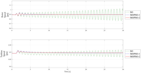
Figure 11.
Performance of the DFIG for voltage sag down to 0.3 p.u.: sub-synchronous speed; mechanical variables.
Figure 12 shows that the tunings managed to stay within the limits of the LVRT curve (see Figure 5). Similarly, the MOPSO-1 and MOPSO-2 tunings showed very similar peaks and damping, as well as appropriate post-fault recovery.
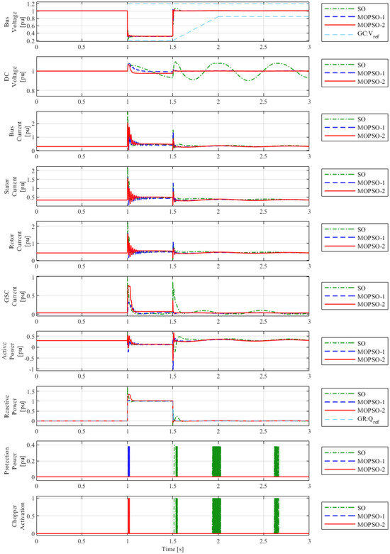
Figure 12.
Performance of the DFIG for voltage sag down to 0.3 p.u.: sub-synchronous speed; electrical variables.
Due to the operation of the DFIG at a lower wind speed (compared to the tuning tests), the peaks of the terminal, stator, rotor and converter currents were lower. Additionally, during the fault period, for a few moments, the DFIG consumed active power from the grid.
The MOPSO-1 and MOPSO-2 tunings achieved an acceptable tracking of the reactive-power reference during and after the fault period.
When the speed was sub-synchronous, due to the lower peak value of the DC-link voltage during the fault, the protection was not triggered by the MOPSO-2 tuning. Therefore, for this lower wind speed, only the MOPSO-1 tuning dissipated power through the protection. This reinforces the fact that with the joint tuning of the PI controllers of the converter and the DC Chopper, better performance of the protection system can be achieved.
Based on the results presented in this subsection, it is understood that the MOPSO-1 and MOPSO-2 tunings also met the performance and stability requirements when the rotor of the DFIG rotated at sub-synchronous speeds.
It was observed that the SO tuning failed to meet the performance and stability requirements.
8.2. Test for Wind Profile
For the last test, the DFIG wind turbine was subjected to a different operating condition. In this case, its performance was tested with the wind profile shown in Figure 13.
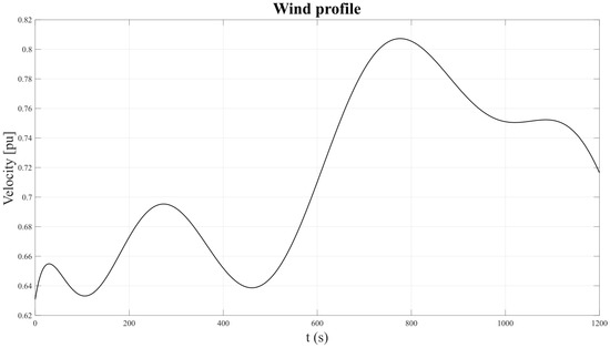
Figure 13.
Wind profile [26].
It can be observed that the profile exhibited various peaks and valleys, as well as maximum and minimum values that were widely spaced. Additionally, it presented a curve with high-amplitude variations, showing the DFIG behavior under a very different condition from the tuning scenario.
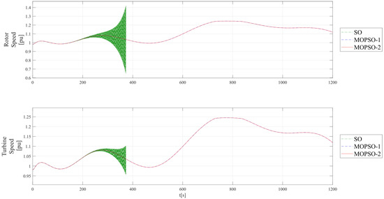
Figure 14.
Performance of the DFIG for wind profile: mechanical variables.
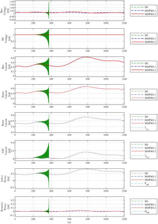
Figure 15.
Performance of the DFIG for wind profile: electrical variables.
The DFIG wind turbine achieved tracking of references and oscillation damping only with the tunings obtained from the MOPSO algorithm (MOPSO-1 and MOPSO-2).
Therefore, with the parameter values of the PI controllers from Table 4 and Table 6, respectively, good performance was achieved with damping of electrical and mechanical quantities.
On the other hand, the behavior of the wind farm with the SO tuning showed undamped oscillations after the second peak of the wind profile (after 200 s), and these oscillations continued to increase until the simulation was interrupted due to the unstable behavior of the DFIG.
It was clarified that, for the wind profile test, there is no need to monitor the protections, as the protection system only operates in the case of a fault.
Observing the results presented in this section, it is possible to understand that the tunings obtained with the MOPSO algorithm can also be used for conditions different from those of tuning.
9. Conclusions
This research sought to incorporate the dynamics of reactive-current injection and DC-Chopper protection during the tuning process of the DFIG-wind-turbine control system in fault conditions with the Multi-Objective-PSO algorithm.
Tunings obtained with the MOPSO algorithm, using sequential and simultaneous tuning strategies, showed better performance than the SO method, both in electrical quantity behavior and in the damping of the mechanical variables. The developed Multi-Objective-PSO algorithm could reach the pre-established requirements, and thus achieved good dynamic performance of the DFIG wind turbine during faults, even with reactive-current injection, as well as in the presence of DC-Chopper protection.
In addition, when the DFIG wind turbine was subjected to an electrical fault, the tuning conditions were very important for the performance and damping of the oscillations of their electrical and mechanical variables. Comparing the proposed tuning methods to the Multi-Objective-PSO, it was observed that sequential tuning (Method 1: MOPSO-1) showed a better performance in relation to the reactive-current injection and lower amplitude deviations of the electrical quantities during and after the fault period. On the other hand, simultaneous tuning of the PIs (Method 2: MOPSO-2) reached faster damping of the mechanical oscillations and better performance of the protection system.
These differences are attributed to the tuning process, because in the first step of Method 1, where the converter controllers were tuned, the fault was not very severe and, therefore, the algorithm prioritized, following the reactive power reference. However, in Method 2, the fault was more severe, the protection system was triggered and the oscillations were higher and, therefore, the algorithm prioritized better damping of the mechanical oscillations and the performance of the protection system.
In conclusion, the dynamics of the protection system and the reactive-current injection are very important and must be incorporated during the tuning process of the DFIG wind turbine.
Author Contributions
Conceptualization, methodology and validation, M.E.B.A., D.V.C., R.R. and R.M.M.; formal analysis, M.E.B.A., D.V.C., R.R. and R.M.M.; investigation, M.E.B.A., D.V.C., R.R., R.M.M. and P.T.d.G.; resources, D.V.C. and T.G.J.; data curation, M.E.B.A., D.V.C., R.R., R.M.M. and P.T.d.G.; writing—original draft preparation, M.E.B.A.; writing—review and editing, M.E.B.A., D.V.C., R.R., R.M.M. and P.T.d.G.; supervision, D.V.C. and T.G.J.; project administration, D.V.C. and T.G.J.; funding acquisition, D.V.C., R.R., R.M.M. and T.G.J. All authors have read and agreed to the published version of the manuscript.
Funding
The authors acknowledge the financial support of the São Carlos School of Engineering—University of São Paulo (USP), the Western Paraná State University (UNIOESTE), and especially to the Itaipu Technological Park Foundation (FPTI) for funding this publication.
Data Availability Statement
Data are contained within the article.
Acknowledgments
The authors wish to express their gratitude to the Itaipu Technological Park Foundation for providing the infrastructure used in this study.
Conflicts of Interest
The authors declare no conflict of interest.
Abbreviations
The following abbreviations are used in this manuscript:
| DC | Direct Current |
| DFIG | Doubly Fed Induction Generator |
| GSC | Grid-Side Converter |
| GC | Grid Code |
| IAE | Integral Absolute Error |
| K | proportional gain |
| LVRT | Low-Voltage Ride Through |
| MOPSO | Multi-Objective-Particle-Swarm Optimization |
| MPPT | Maximum-Power-Point Tracking |
| OF | Objective Functions |
| PI | Proportional–Integral |
| PLL | Phase-Locked Loop |
| PSO | Particle-Swarm Optimization |
| PWM | Pulse-Width Modulation |
| RSC | Rotor-Side Converter |
| SO | Symmetrical Optimum |
| Ti | Integral Time |
References
- Anaya-Lara, O.; Jenkins, N.; Ekanayake, J.; Cartwright, P.; Hughes, M. Wind Energy Generation: Modelling and Control; John Wiley and Sons, Ltd.: Hoboken, NJ, USA, 2009; Volume 1. [Google Scholar]
- Kamel, O.M.; Diab, A.A.Z.; Do, T.D.; Mossa, M.A. A Novel Hybrid Ant Colony-Particle Swarm Optimization Techniques Based Tuning STATCOM for Grid Code Compliance. IEEE Access 2020, 8, 41566–41587. [Google Scholar] [CrossRef]
- Mansouri, M.M.; Nayeripour, M.; Negnevitsky, M. Internal electrical protection of wind turbine with doubly fed induction generator. Renew. Sustain. Energy Rev. 2016, 55, 840–855. [Google Scholar] [CrossRef]
- Mosaad, M.I.; Abu-siada, A.; El-Naggar, M. Application of Superconductors to Improve the Performance of DFIG-Based WECS. IEEE Access 2019, 7, 103760–103769. [Google Scholar] [CrossRef]
- Haidar, A.M.A.; Member, S.; Muttaqi, K.M.; Member, S. A Coordinated Control Approach for DC link and Rotor Crowbars to Improve Fault Ride-Through of DFIG-Based Wind Turbine. IEEE Trans. Ind. Appl. 2017, 53, 4073–4086. [Google Scholar] [CrossRef]
- Aguilar, M.E.B.; Coury, D.V.; Reginatto, R.; Monaro, R.M. Multi-objective PSO applied to PI control of DFIG wind turbine under electrical fault conditions. Electr. Power Syst. Res. 2020, 180, 106081. [Google Scholar] [CrossRef]
- Alhato, M.M.; Bouallègue, S. Direct Power Control Optimization for Doubly Fed Induction Generator Based Wind Turbine Systems. Math. Comput. Appl. 2019, 24, 77. [Google Scholar] [CrossRef]
- Ahmed, G.E.; Mohmed, Y.S.; Kamel, O.M. Optimal STATCOM controller for enhancing wind farm power system performance under fault conditions. In Proceedings of the 18th International Middle-East Power Systems Conference, MEPCON 2016, Cairo, Egypt, 27–29 December 2016. [Google Scholar] [CrossRef]
- Abd, M.K.; Cheng, S.J.; Sun, H.S. A new MBF-PSO for improving performance of DFIG connected to grid under disturbance. In Proceedings of the 2016 IEEE PES Asia-Pacific Power and Energy Engineering Conference (APPEEC), Xi’an, China, 25–28 October 2016. [Google Scholar] [CrossRef]
- Elgammal, A.A.A. Optimal design of PID controller for Doubly-Fed induction generator-based wave energy conversion system using multi-objective particle swarm optimization. J. Technol. Innov. Renew. Energy 2014, 3, 21–30. [Google Scholar] [CrossRef]
- Hamid, B.; Hussain, I.; Iqbal, S.J.; Singh, B.; Das, S.; Kumar, N. Optimal MPPT and BES Control for Grid-Tied DFIG-Based Wind Energy Conversion System. IEEE Trans. Ind. Appl. 2022, 58, 7966–7977. [Google Scholar] [CrossRef]
- Jiang, F.; Zhang, C.; Li, T.; Xiao, H.; Cui, D. Reactive Power Optimization Strategy of Wind Farm based on Particle Swarm Optimization Algorithm. In Proceedings of the 2022 IEEE Transportation Electrification Conference and Expo, Asia-Pacific, ITEC Asia-Pacific 2022, Haining, China, 28–31 October 2022. [Google Scholar] [CrossRef]
- Anilkumar, R.; Devriese, G.; Srivastava, A.K. Voltage and Reactive Power Control to Maximize the Energy Savings in Power Distribution System with Wind Energy. IEEE Trans. Ind. Appl. 2018, 54, 656–664. [Google Scholar] [CrossRef]
- Pereira, R.M.M.; Pereira, A.J.C.; Ferreira, C.M.; Barbosa, F.P.M. Influence of Crowbar and Chopper Protection on DFIG during Low Voltage Ride Through. Energies 2018, 11, 885. [Google Scholar] [CrossRef]
- Debre, P.; Juneja, R.; Tutakane, D.; Ramteke, M. Overvoltage protection scheme for back to back converter of grid connected DFIG. In Proceedings of the IECON 2015—41st Annual Conference of the IEEE Industrial Electronics Society, Yokohama, Japan, 9–12 November 2015. [Google Scholar] [CrossRef]
- Islam, R.; Ajom, G.; Sheikh, M.R.I. Application of DC Chopper to Augment Fault Ride Through of DFIG Based Wind Turbine. In Proceedings of the 2nd International Conference on Electrical & Electronic Engineering (ICEEE), Rajshahi, Bangladesh, 27–29 December 2017. [Google Scholar] [CrossRef]
- Zamzoum, O.; El Mourabit, Y.; Derouich, A.; El Ghzizal, A. Study and implementation of the MPPT strategy applied to a variable speed wind system based on DFIG with PWM-vector control. In Proceedings of the 2016 International Conference on Electrical Sciences and Technologies in Maghreb, CISTEM 2016, Marrakech & Bengrir, Morocco, 26–28 October 2016. [Google Scholar] [CrossRef]
- Ackermann, T. Wind Power in Power Systems; John Wiley and Sons, Ltd.: Stockholm, Sweden, 2005; Volume 140. [Google Scholar]
- Prasanthi, E.; Shubhanga, K.N. Stability analysis of a grid connected DFIG based WECS with two-mass shaft modeling. In Proceedings of the 2016 IEEE Annual India Conference, INDICON 2016, Bangalore, India, 16–18 December 2016. [Google Scholar] [CrossRef]
- El-jalyly, A.; Derri, M.; Haidi, T.; Janyene, A. Modeling and Control of a DFIG for wind Turbine Conversion System using Back-to-back PWM Converters. In Proceedings of the 2019 7th International Renewable and Sustainable Energy Conference (IRSEC), Agadir, Morocco, 27–30 November 2019. [Google Scholar] [CrossRef]
- National Electrical System Operator (ONS). Submodule 3.6—Minimum Technical Requirements for Connection to Transmission Installations; Technical Report; ANNEL–ONS: Rio de Janeiro, Brazil, 2019. (In Portuguese) [Google Scholar]
- Asif, M.; Bux, R.; Memon, R.A. Improved RSC-GSC decoupled and LVRT Control Strategies of DFIG-Based Wind Turbine. In Proceedings of the 2018 International Conference on Electrical Engineering, ICEE, Lahore, Pakistan, 15–16 February 2018. [Google Scholar] [CrossRef]
- Ogata, K. Ingeniería de Control Moderna, 5th ed.; Pearson: Madrid, Spain, 2003. [Google Scholar] [CrossRef]
- Astrom, K.J.; Hägglund, T. PID Controllers: Theory, Design and Tuning, 2nd ed.; Instrument Society of America: Lung, Sweden, 1995. [Google Scholar]
- Queval, L.; Ohsaki, H. Back-to-back converter design and control for synchronous generator-based wind turbines. In Proceedings of the 2012 International Conference on Renewable Energy Research and Applications (ICRERA), Nagasaki, Japan, 11–14 November 2012. [Google Scholar] [CrossRef]
- Alcântara, Pedro Victor Rodrigues. Development of a DFIG Simulator Applied to Different Wind Profiles; Final Project of the Course; Federal University of Ceará (UFC): Fortaleza, Brazil, 2019. (In Portuguese) [Google Scholar]
Disclaimer/Publisher’s Note: The statements, opinions and data contained in all publications are solely those of the individual author(s) and contributor(s) and not of MDPI and/or the editor(s). MDPI and/or the editor(s) disclaim responsibility for any injury to people or property resulting from any ideas, methods, instructions or products referred to in the content. |
© 2023 by the authors. Licensee MDPI, Basel, Switzerland. This article is an open access article distributed under the terms and conditions of the Creative Commons Attribution (CC BY) license (https://creativecommons.org/licenses/by/4.0/).