Low-Carbon Optimal Scheduling of Integrated Energy System Considering Multiple Uncertainties and Electricity–Heat Integrated Demand Response

Abstract

To realize the low-carbon operation of integrated energy systems (IESs), this paper proposes a low-carbon optimal scheduling method. First of all, considering the integrated demand response of price-based electricity and heating, an economic scheduling model of the IES integrated demand response based on chance-constrained programming is proposed to minimize the integrated operating cost in an uncertain environment. Through the comprehensive demand response model, the impact of the demand response ratio on the operating economy of the IES is explored. Afterward, the carbon emission index is introduced, and gas turbines and energy storage devices are used as the actuators of multi-energy coupling to further explore the potential interactions between the coupling capacities of various heterogeneous energy sources and carbon emissions. Finally, the original uncertainty model is transformed into a mixed-integer linear-programming model and solved using sequence operation theory and the linearization method. The results show that the operating economy of the IES is improved by coordinating the uncertainty of the integrated demand response and renewable energy. In addition, the tradeoff between the working economy and reliability of the EIS can be balanced via the setting of an appropriate confidence level for the opportunity constraints.

1. Introduction

To fulfill the goal of Carbon Peak and Carbon Neutrality, traditional power systems are changing into integrated energy systems (IESs), with a large number of distributed energy sources (DERs) with uncertainties, such as wind power and photovoltaic (PV) power generation [1,2,3]. At the same time, many time-varying loads, like electric vehicles (EVs), also introduce uncertainties into the IES and bring new challenges to its optimal scheduling [4,5,6]. As a supply and marketing system, the IES can couple different energy structures, including electricity distribution systems, gas networks and heating systems. The establishment of an IES in an uncertain environment is crucial to the realization of China’s low-carbon commitment. Therefore, the optimal scheduling of the IES has attracted the broad interest of many researchers and has become a research hotspot [7,8,9].

Currently, many studies report on dealing with the multi-uncertainties of the IES. The problem is that some DERs, like wind and solar energy, are intermittent and have intrinsic uncertainty, which may threaten the safe operation of the network. To overcome this deficiency, an economic operation strategy for a hydrogen-centric IES, which considers the uncertainty of the PV output, is proposed in [10]. In [11], a segmentation method is proposed to model the power output and load demand of the DERs to ensure system safety. To further reveal the impact of the PV intermittence on the IES, a risk-aware energy-scheduling and stochastic optimization method has been proposed by Liu et al. [12]. In [13], a method combining machine learning and distributed robust optimization (DRO) is proposed, which can obtain stable decision solutions in terms of uncertainty assumptions. Actually, for IESs, the greatest challenge lies in balancing the uncertainties in both the source and load sides efficiently and economically. Therefore, optimal scheduling models or strategies optimized with robust methods are proposed [14,15,16]. To solve the problem of the insufficient operational flexibility of the IES, a robust stochastic optimization model of the IES with advanced adiabatic compressed-air energy storage is proposed in [17], and a data-driven stochastic collaborative optimization model for a power–gas IES was developed by Zheng et al. in [16]. In addition, to minimize the overall energy consumption cost, Zhao et al. [18] propose a stochastic scheduling expectation model, while Cui et al. [19] establish a multi-objective optimal scheduling model under multi-uncertainties.

With the development and expansion of the energy market, the comprehensive demand response and carbon trading have become hot topics. To achieve the low-carbon and economic operation of the IES and thereby improve the optimization management level, a multi-time-scale, low-carbon, optimal operation strategy considering the DRO of electricity, gas, heat and hydrogen and the stepped carbon emission charging mechanism are proposed in [20]. Moreover, an accurate model of typical controllable loads and an uncertainty model for the response of transferable and replaceable loads are also introduced in [21,22,23].

According to the temperature perception fuzziness of heat users and the thermal inertia of heating buildings, an adjustable heat load response model considering the uncertainty of the light intensity has been established, and an optimal scheduling strategy based on comprehensive DRO has been developed [24,25]. To cope with the uncertainty of the price and demand of electricity, a scenario-oriented method is used in [26]. Similarly, the demand response is also unneglectable for the schedulable microgrid, and model predictive control (MPC) is commonly used [27,28,29].

The abovementioned literature has designed and characterized the uncertainties of the IES model from different aspects. However, chance-constrained programming has not been used to model the uncertainty of IES scheduling. Chance-constrained programming has received extensive attention in solving the uncertainty in IES operations for its ability to deal with the uncertainty more appropriately, especially under probability constraints.

Although there has been a lot of research on the optimal scheduling of integrated energy systems, and the basic optimal scheduling problem has been solved, the following research gap in this field still exists: the uncertainties of the DERs and time-varying loads have a significant impact on the optimal scheduling strategy. To ensure the operational reliability of the integrated energy system, previous works have mainly considered the rotating reserve capacity as a deterministic constraint related to the minimum reserve required by the system. However, if all uncertainties, such as fluctuations in the DERs, power load and system faults, are considered, how to skillfully describe the uncertainty problem and further deal with the constraints is still challenging. In response to this challenge, this paper constructs a response scheduling model for the integrated electricity–heat demand of the IES based on chance-constrained planning in an uncertain environment. The main contributions are as follows:

• Combined with the IES under multi-uncertainties, the price-based comprehensive demand response model and the model of DERs with uncertainty are established. Furthermore, considering the economy and decarbonization of the system, an integrated demand response scheduling model based on chance-constrained programming in an uncertain environment is constructed;
• The sequence operation theory is used to transform the opportunity constraint into a deterministic constraint. Then, the original model is transformed into a mixed-integer linear-programming model via a linearization method, which has high effectiveness for solving the opportunity constraint;
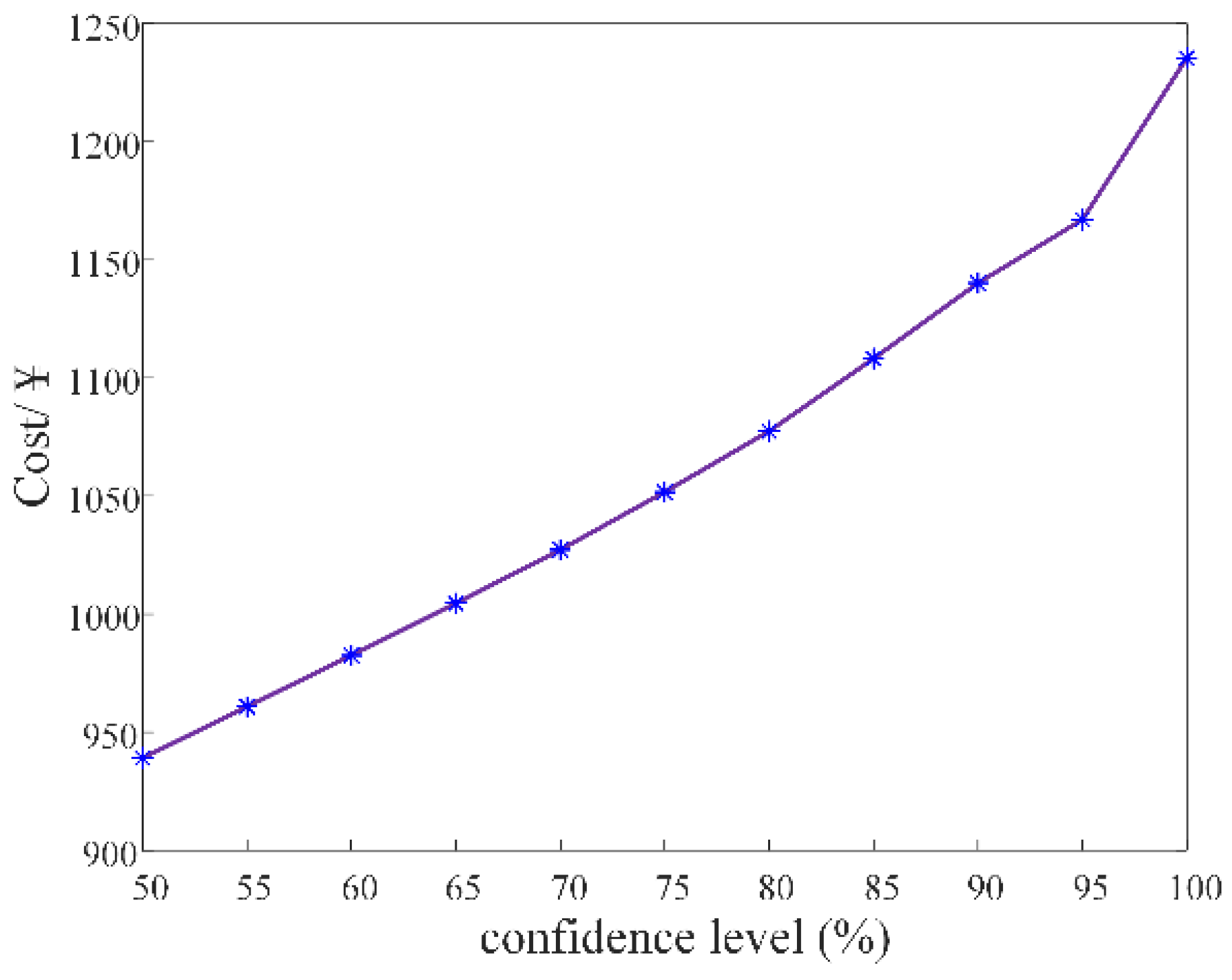
• The effectiveness of coordinating the integrated demand response and the uncertainty of the DERs in reducing carbon emissions and improving the economic efficiency of integrated energy systems is verified with simulation. By setting the right confidence level, a balance can be achieved between the operational economics and operational reliability of an IES.

The rest of this paper is organized as follows: Section 2 introduces the demand response and uncertainty modeling of the IES. Section 3 elaborates on the optimization scheduling model and solution of the IES. Section 4 verifies the effectiveness of the proposed scheme by comparing the results of different real-case scenarios. Finally, the conclusions are drawn in Section 5.

2. IES Model with Multi-Uncertainties

This section describes the system architecture of the proposed IES scheduling model and accurately models the mathematical models of each link in the IES.

2.1. Architecture of the IES

The system architecture of the electricity–heat IES considering multi-uncertainties in this paper is shown in Figure 1. The power sources in the IES mainly include uncertain sources, like wind turbines (WTs) and PV panels, a traditional thermal power (TP) plant, combined heat and power (CHP), a gas turbine (GT), a gas boiler (GB), a lithium bromide refrigerator (LBR), an EV-charging station (EVCS), electrical energy storage (EES), thermal energy storage (TES) and an air tank (AT). The loads are the electric load (EL) and heat load (HL), according to the energy properties. According to the actual situation of energy consumption, loads can be divided into residential loads, industrial loads and EVs.

Figure 1. System architecture of electricity–heat IES.

In Figure 1, the gas turbine and energy storage device are used as the connection carriers of different energy sources. The power grid and heat supply network are coupled to optimize and coordinate the production, transmission, distribution and consumption of various energy sources. The power load includes a constant load, interruptible load and time-shifting load, while the electric power is provided by the power grid, DERs, gas turbine and EES devices. The thermal load also includes a constant load and time-shifting load, while the thermal energy is provided by the power grid, DERs, bromine cooler and thermal energy storage devices. EVs are devices that can obtain electricity from power grids, DERs and gas turbines. Considering the randomness and intermittence of the DERs, to suppress their uncertainty, the IES improves the flexibility and reliability of the system by reserving a certain amount of the spinning-reserve capacity from the power grid, gas turbine and EES in advance, which helps the system obtain the maximum benefit.

2.2. Price-Based Demand Response

The demand response of the IES mainly includes the electricity price demand response and incentive demand response [30,31,32]. The price-based demand response focuses on resources that cannot be directly dispatched, mainly including the EV-charging and other electricity consumption behaviors of users. Adjusting the electricity price at the load peak and valley can help stabilize the system load. The demand response elasticity coefficient can be used to describe the user response to the electricity price, as in Equation (1):

$$\epsilon =\frac{\Delta P_{t,t+\Delta t}}{P_t}·\frac{q_t}{\Delta q_{t,t+\Delta t}}$$

(1)

where P_t and q_t are the electrical power and electricity price in the previous t period, respectively, and ΔP_t,t+Δt and Δq_t,t+Δt are the changes in the electrical power and electricity price after the demand response.

By analyzing the load curve, a reasonable time-of-use price can effectively reduce the difference between the load peak and valley. According to the load curve, the users’ loads will be divided into three periods: the load peak, normal period and load valley. The electricity prices of these periods are set for demand-side response analysis using Equations (2) and (3):

$$\left[\begin{array}{c}\Delta P_F\\ \Delta P_P\\ \Delta P_G\end{array}\right]=\left[\begin{array}{ccc}{\epsilon }_{\mathrm{F}\mathrm{F}}& {\epsilon }_{\mathrm{F}\mathrm{P}}& {\epsilon }_{\mathrm{F}\mathrm{G}}\\ {\epsilon }_{\mathrm{P}\mathrm{F}}& {\epsilon }_{\mathrm{PP}}& {\epsilon }_{PG}\\ {\epsilon }_{\mathrm{G}\mathrm{F}}& {\epsilon }_{\mathrm{GP}}& {\epsilon }_{\mathrm{G}\mathrm{G}}\end{array}\right]\left[\begin{array}{c}\Delta q_F\\ \Delta q_P\\ \Delta q_G\end{array}\right]$$

(2)

$$E=\left[\begin{array}{ccc}{\epsilon }_{\mathrm{F}\mathrm{F}}& {\epsilon }_{\mathrm{F}\mathrm{P}}& {\epsilon }_{\mathrm{F}\mathrm{G}}\\ {\epsilon }_{\mathrm{P}\mathrm{F}}& {\epsilon }_{\mathrm{PP}}& {\epsilon }_{PG}\\ {\epsilon }_{\mathrm{G}\mathrm{F}}& {\epsilon }_{\mathrm{GP}}& {\epsilon }_{\mathrm{G}\mathrm{G}}\end{array}\right]$$

(3)

where ΔP and Δq are the change matrix of the average demands of different periods and the electricity price, respectively; E is the demand elasticity matrix; ε_FF, ε_PP and ε_GG are the self-elastic coefficients; and ε_FG, ε_PG and ε_FP are the mutual-elasticity coefficients, respectively.

2.3. Demand Response Modeling of Electricity–Heat Loads

In the IES, the main loads include rigid loads and flexible loads [33,34]. The flexible loads can participate in the demand response to control the total load profile of the system, improve the energy consumption quality of the system and reduce the cost. The flexible loads can be divided into reducible loads and time-shifting loads, according to the regulation mode.

2.3.1. Interruptible Electrical Load

The interruptible electrical load has a quick response to the system’s demand. On the premise that users sign agreements with the power sector, it can promote the balance between the supply and demand of the system during peak power consumption hours, while considering the system’s reliability. The specific mathematical model for the interruptible electrical load can be expressed as Equation (4):

$$P_t^{\mathrm{IL}}=\left(1-\theta \right)P_{t,\max }^{\mathrm{IL}}, 0\le \theta \le 1$$

(4)

where $P_t^{\mathrm{TL}}$ and $P_{t,\max }^{\mathrm{TL}}$ are, respectively, the maximum value of the interruptible load power and its maximum value in period t, while θ represents the reduction ratio of the interruptible load in period t.

2.3.2. Time-Shifting Electrical and Thermal Loads

There are partial loads in IESs that have load transfer capabilities, and these loads can be divided into three categories. The first category is continuous-production and -operation enterprises, such as the chemical, metallurgy and steel industries, which can only adjust the production process, but the change in the process is very limited. The second category is high-energy-consuming enterprises, characterized by the fact that the electricity costs account for a large proportion of the enterprise operating costs and are extremely sensitive to energy prices. The third category is small- and medium-sized enterprises with relatively flexible production processes, which are characterized by the flexible arrangement of the production plans in low-electricity-price periods. In addition, the residential electricity consumption is smaller than the industrial and commercial energy consumption, but the electricity consumption of EVs, mobile phones and household appliances can be shifted to night to a certain extent. The specific mathematical model of transferable electric or thermal loads can be modeled as Equations (5) and (6):

$$\left\{\begin{array}{l}{P}_{t,\mathrm{EL},\min }^{\mathrm{TS}}\le P_{t,\mathrm{EL}}^{\mathrm{TS}}\le P_{t,\mathrm{EL},\max }^{\mathrm{TS}}\\ P_{t,\mathrm{HL},\min }^{\mathrm{TS}}\le P_{t,\mathrm{HL}}^{\mathrm{TS}}\le P_{t,\mathrm{HL},\max }^{\mathrm{TS}}\end{array}\right.$$

(5)

$$\left\{\begin{array}{l}{\displaystyle \sum _{t=1}^T{P}_{t,\mathrm{EL}}^{\mathrm{TS}}=0}\\ {\displaystyle \sum _{t=1}^T{P}_{t,\mathrm{HL}}^{\mathrm{TS}}=0}\end{array}\right.$$

(6)

where $P_{t,\mathrm{EL}}^{\mathrm{TS}}$ and $P_{t,\mathrm{HL}}^{\mathrm{TS}}$ are the transferable power of the electrical load and thermal load in period T, respectively; $P_{t,\mathrm{EL},\min }^{\mathrm{TS}}$ and $P_{t,\mathrm{EL},\max }^{\mathrm{TS}}$ are the minimum and maximum values of the transferable power of the electric load in period T; $P_{t,\mathrm{HL},\min }^{\mathrm{TS}}$ and $P_{t,\mathrm{HL},\max }^{\mathrm{TS}}$ are the minimum and maximum values of the transferable power of the heat load in period T.

From Equation (6), it is clear that the total transferable electric or thermal load in a dispatching period is 0, which means that the total loads transferred in and out of the system are equal.

2.4. Uncertainty Modeling of DERs

2.4.1. Probability Model of Wind Power Generation

According to statistics, the wind speed follows the Weibull distribution at a certain time. Therefore, the wind power output probability density function (PDF) can be derived from the wind speed PDF and the output power as Equation (7). The specific derivation process of the probability density function for the fan output is in the Appendix A.

$$f_1\left(P_{WT}\right)=\left\{\begin{array}{l}\left(kc{v}_{\mathrm{ci}}/a\times P^{*}\right){\left[\left(\left(1+c{P}_{\mathrm{WT}}/P^{*}\right)v_{\mathrm{ci}}\right)/a\right]}^{k-1}\\ \times \exp \left\{-{\left[\left(\left(1+c{P}_{\mathrm{WT}}/P^{*}\right)v_{\mathrm{ci}}\right)/a\right]}^k\right\}\\ ,P_{\mathrm{WT}}\in \left[0,P^{*}\right] \\ 0 ,\mathrm{otherwise} \end{array}\right.$$

(7)

where c = (v* − v_ci)/v_ci, and v is the actual wind speed; k is the shape coefficient (dimensionless), which describes the PDF shape of the wind speed; a is the scaling factor; v_ci is the cut-in wind speed; v_co is the cut-out wind speed; v* is the rated wind speed; P* is the rated output power of the wind generator; P_WT is the output of the wind power.

2.4.2. Probability Model of PV Power Generation

According to statistics, the solar illumination intensity meets the beta distribution, and the PDF of the PV output can be derived from the PDF of the solar illumination intensity and PV output power, as in Equation (8). The specific derivation process of the probability density function for the photovoltaic output is shown in the Appendix A.

$$f\left(P_{\mathrm{PV}}\right)=\frac{\Gamma \left(\alpha \right)+\left(\beta \right)}{\Gamma \left(\alpha \right)\Gamma \left(\beta \right)}{\left(\frac{P_{\mathrm{PV}}}{P_{\mathrm{PV},\max }}\right)}^{\alpha -1}{\left(1-\frac{P_{\mathrm{PV}}}{P_{\mathrm{PV},\max }}\right)}^{\beta -1}$$

(8)

where Γ is the gamma function; α and β are the shape factors of the beta distribution curve, respectively; P_PV and P_PV,max are the actual PV output and its maximum value, respectively.

2.5. Coupling Equipment Modeling

2.5.1. Model of the CHP Unit

The CHP unit is an energy supply system that integrates the power generation and heat supply. Typical CHP units mainly include gas turbines and bromine coolers. The mathematical model of a CHP unit is expressed as Equation (9) [35]:

$$\left\{\begin{array}{l}{Q}_t^{\mathrm{GT}}=P_t^{\mathrm{GT}}\left(1-{\mu }_{\mathrm{loss}}\right)\\ P_t^{\mathrm{LB}}=Q_t^{\mathrm{GT}}{\eta }_{\mathrm{LB}}^{\mathrm{rec}}{\lambda }_{\mathrm{LB}}\end{array}\right.$$

(9)

where $Q_t^{\mathrm{GT}}$ is the residual heat of the gas released from the gas turbine; $P_t^{\mathrm{GT}}$ is the output of the gas turbine; μ_loss is the heat dissipation loss coefficient of the gas turbine; $P_t^{\mathrm{LB}}$ is the thermal power of the bromine cooler; η_rec and λ_LB are the waste heat recovery efficiency and the thermal efficiency of the bromine cooler.

2.5.2. Electrical and Thermal Energy Storage Model

To reduce the influence of uncertain factors in the IES, it is necessary to introduce electric energy storage and thermal energy storage equipment. The operation modes of the energy storage devices are the same. Taking electric energy storage as an example, its mathematical model can be denoted as Equation (10):

$$\left\{\begin{array}{l}{D}_{t+1,\mathrm{ESS}}=D_{t,\mathrm{ESS}}+(P_{t,\mathrm{ESS}}^{\mathrm{CH}}{\eta }_{\mathrm{ESS}}^{\mathrm{CH}}-P_{t,\mathrm{ESS}}^{\mathrm{DC}}/{\eta }_{\mathrm{ESS}}^{\mathrm{DC}})\Delta t\\ {\displaystyle \sum _{t=1}^T(P_{t,\mathrm{ESS}}^{\mathrm{CH}}{\eta }_{\mathrm{ESS}}^{\mathrm{CH}}-P_{t,\mathrm{ESS}}^{\mathrm{DC}}/{\eta }_{\mathrm{ESS}}^{\mathrm{DC}})}\Delta t=0\end{array}\right.$$

(10)

where D_t,ESS and D_t+1,ESS are the energy of the electric energy storage device at time t and time t + 1, respectively; $D_{t,\mathrm{ESS}}^{\mathrm{CH}}$ and $D_{t,\mathrm{ESS}}^{\mathrm{DC}}$ are the charging and discharging powers of the electric energy storage; and ${\eta }_{\mathrm{ESS}}^{\mathrm{CH}}$ and ${\eta }_{\mathrm{ESS}}^{\mathrm{DC}}$ are the charging and discharging efficiencies of the electric energy storage, respectively.

3. IES Optimal Scheduling Model with Multi-Uncertainties

This section establishes an IES scheduling model that considers multiple uncertainties, mainly including the objective function, constraint conditions and model solving process.

3.1. Objective Function

The electricity–heat IES in this paper comprehensively considers the cost of the energy, the cost of the system backup, the cost of the energy storage operation and maintenance, the cost of the EV charging, the cost of the carbon trading and the cost of the gas turbine startup and shutdown. The cost function is shown in Equation (11):

$$\min C=\min \left(C_1+C_2+C_3+C_4+C_5+C_6\right)$$

(11)

(1)

Cost of energy

The energy cost of the IES mainly includes the cost of the purchasing power from the power utility for both the electric load and thermal load, which can be expressed as Equation (12):

$$C_1={\displaystyle \sum _{t=1}^T\left[s_{\mathrm{st}\_\mathrm{price},t}·\left(P_t^{\mathrm{GL}}+P_{t,\mathrm{EL}}^{\mathrm{TS}}+P_t^{\mathrm{HL}}-P_{t,\mathrm{HL}}^{\mathrm{TS}}+P_t^{\mathrm{IL}}\right)\right]}$$

(12)

where s_{st_price,t} is the price of the electricity at different times; $P_t^{\mathrm{GL}}$ and $P_t^{\mathrm{HL}}$ are the constant electrical load and thermal load, respectively; $P_{t,\mathrm{EL}}^{\mathrm{TS}}$ and $P_{t,\mathrm{HL}}^{\mathrm{TS}}$ stand for the time-shifting electrical load and thermal load, respectively; $P_t^{\mathrm{IL}}$ is the constant heat load in period t;

(2)

Cost of system backup

The system backup cost mainly considers the operation cost of the power grid, EES and rotating backup reserved by the gas turbine, which can be expressed as Equation (13):

$$C_2={\displaystyle \sum _{t=1}^T\left(\begin{array}{l}{s}_{\mathrm{re}\_\mathrm{price}}^{\mathrm{grid}}·R_t^{\mathrm{grid}}+s_{\mathrm{re}\_\mathrm{price}}^{\mathrm{ESS}}·R_t^{\mathrm{ESS}}\\ +s_{\mathrm{re}\_\mathrm{price}}^{\mathrm{GT}}·R_t^{\mathrm{GT}}\end{array}\right)}$$

(13)

where $s_{\mathrm{re}\_\mathrm{price}}^{\mathrm{grid}}$, $s_{\mathrm{re}\_\mathrm{price}}^{\mathrm{ESS}}$ and $s_{\mathrm{re}\_\mathrm{price}}^{\mathrm{GT}}$ are the unit power reserve prices of the power grid, EES and gas turbine, respectively; $R_t^{\mathrm{grid}}$, $R_t^{\mathrm{ESS}}$ and $R_t^{\mathrm{GT}}$ are the reserve capacities of the power grid, EES and gas turbine, respectively;

(3)

Energy storage operation and maintenance cost

The operation and maintenance cost of the EES is described as Equation (14):

$$C_3={\displaystyle \sum _{t=1}^T{s}_{\mathrm{dp}\_\mathrm{price}}^{\mathrm{ESS}}·P_t^{\mathrm{ESS}}}$$

(14)

where $s_{dp\_\mathit{price}}^{\mathrm{ESS}}$ is the maintenance cost of the EES per unit of power, and $P_t^{\mathrm{ESS}}$ is the EES charging power;

(4)

Cost of EV charging

The cost of EV charging can be denoted as Equation (15):

$$C_4={\displaystyle \sum _{t=1}^T{s}_{\mathit{st}\_\mathit{price},t}·P_t^{\mathrm{EV}}}$$

(15)

where s_{st_price} is the electricity price of EVs at different times, and $P_t^{\mathrm{EV}}$ is the charging power of the EVs;

(5)

Cost of carbon transaction

The cost of the carbon transaction is described as Equation (16):

$$C_5={\displaystyle \sum _{t=1}^T{s}_{{\mathrm{co}}_2}\left(E_{\mathrm{c},t}-D_{\mathrm{c},t}\right)}$$

(16)

where s_{${\mathrm{co}}_2$} is the carbon-trading price, and E_c,t and D_c,t represent the carbon emissions and carbon allocations at different times [36];

(6)

Operating cost of gas turbine:

$$C_6={\displaystyle \sum _{t=1}^T\left[\kappa S_t+U_t\left(\upsilon +\psi P_t^{\mathrm{GT}}\right)\right]}$$

(17)

where S_t and U_t are the startup/shutdown variable and state variable of the gas turbine, respectively; v and ψ stand for the consumption coefficients of the gas turbine; κ is the startup and shutdown cost of the gas turbine.

3.2. Constraint Conditions

3.2.1. Power Supply System Constraints

The constraints of the power supply system constitute the power balance, electric load demand response, grid and gas turbine output, EES charging and discharging powers, EES capacity, EES start and stop states and EV-charging power and capacity.

(1)

Constraints of electric power balance:

$$\left\{\begin{array}{l}{P}_{\mathrm{e}\_\mathrm{source}}=P_{t,\mathrm{EL}}^{\mathrm{grid}}+P_{t,\mathrm{EL}}^{\mathrm{GT}}-P_{t,\mathrm{ESS}}^{\mathrm{CH}}+P_{t,\mathrm{ESS}}^{\mathrm{DC}}+E\left(P_t^{\mathrm{DER}}\right)\\ P_{\mathrm{e}\_\mathrm{load}}=P_{t,\mathrm{EL}}^{\mathrm{GL}}+P_t^{\mathrm{EV}}+P_{t,\mathrm{EL}}^{\mathrm{TS}}+P_t^{\mathrm{CL}}-P_t^{\mathrm{IL}}\\ P_{\mathrm{e}\_\mathrm{source}}=P_{\mathrm{e}\_\mathrm{load}}\end{array}\right.$$

(18)

where P_{e_source} and P_{e_load} are the output of the power source and the total electrical load; $P_{t,\mathrm{EL}}^{\mathrm{grid}}$ and $P_{t,\mathrm{EL}}^{\mathrm{GT}}$ are the power of grid r and the gas turbine; $P_{t,\mathrm{ESS}}^{\mathrm{CH}}$ and $P_{t,\mathrm{ESS}}^{\mathrm{DC}}$ are the EES charging and discharging powers; E($P_t^{\mathrm{DER}}$) is the expected value of the DERs; $P_{t,\mathrm{EL}}^{\mathrm{GL}}$, $P_t^{\mathrm{EV}}$, $P_t^{\mathrm{TSL}}$, $P_t^{\mathrm{CL}}$ and $P_t^{\mathrm{IL}}$ are the power consumption of the constant electric load, EVs, time-shifting load, controllable load and interruptible load, respectively;

(2)

Constraints of grid output and gas turbine output

Assuming that $P_{\max }^{\mathrm{grid}}$ and $P_{\min }^{\mathrm{grid}}$ are the upper and lower limits of the grid output, respectively, the constraints of the grid output and gas turbine output can be described as follows:

$$\left\{\begin{array}{l}{P}_{\min }^{\mathrm{grid}}\le P_t^{\mathrm{grid}}\le P_{\max }^{\mathrm{grid}}\\ P_{\min }^{\mathrm{GT}}\le P_t^{\mathrm{GT}}\le P_{\max }^{\mathrm{GT}}\end{array}\right.$$

(19)

where $P_{\mathit{max}}^{GT}$ and $P_{\mathit{min}}^{GT}$ stand for the upper and lower limits of the gas turbine output, respectively;

(3)

Constraints of EES charging and discharging powers

Similarly, if $P_{t,\mathrm{ESS}}^{\mathrm{CH}}$ and $P_{t,\mathrm{ESS}}^{\mathrm{DC}}$ stand for the charging and discharging powers of the EES, the constraints can be described as Equation (20):

$$\left\{\begin{array}{l}0\le P_{t,\mathrm{ESS}}^{\mathrm{CH}}\le P_{\mathrm{ESS},\max }^{\mathrm{CH}}\\ 0\le P_{t,\mathrm{ESS}}^{\mathrm{DC}}\le P_{\mathrm{ESS},\max }^{\mathrm{DC}}\end{array}\right.$$

(20)

where $P_{\mathrm{ESS},\mathit{max}}^{\mathrm{CH}}$ and $P_{\mathrm{ESS},\mathit{max}}^{\mathrm{DC}}$ are the upper limits of the EES charging and discharging powers, respectively;

(4)

Constraints of EES capacity and EES state

Considering C_t,ESS as the capacity of the EES, while C_ESS,max and C_ESS,min stand for the upper and lower limits of the EES capacity, respectively, the constraints of the EES capacity and EES state can be described as Equation (21):

$$\left\{\begin{array}{l}{C}_{\mathrm{ESS},\min }\le C_{t,\mathrm{ESS}}\le C_{\mathrm{ESS},\max }\\ C_{t,\mathrm{ESS}}^{\mathrm{SATART}}=C_{t,\mathrm{ESS}}^{\mathrm{END}}=C_{\mathrm{ESS}}^{*}\end{array}\right.$$

(21)

where $C_{\mathrm{ESS}}^{*}$ is the initial EES limit, and $C_{t,\mathrm{ESS}}^{\mathrm{START}}$ and $C_{t,\mathrm{ESS}}^{\mathrm{END}}$ are the initial and end EES capacities, respectively;

(5)

Constraints of EV-charging power and capacity

Let $P_{k,t,\mathrm{EV}}^{\mathrm{CH}}$ and $P_{k,\mathrm{EV},\max }^{\mathrm{CH}}$ denote the charging power and its maximum value of the k-th EV at time t, and let $C_{k,t}^{\mathrm{EV}}$, $C_{k,\max }^{\mathrm{EV}}$ and $C_{k,\min }^{\mathrm{EV}}$ be the battery capacity and the upper and lower limits of the battery capacity of the EV. The constraints of the EV-charging power and capacity can be described as Equation (22):

$$\left\{\begin{array}{l}0\le P_{k,t,\mathrm{EV}}^{\mathrm{CH}}\le P_{k,\mathrm{EV},\max }^{\mathrm{CH}}\\ C_{k,\min }^{\mathrm{EV}}\le C_{k,t}^{\mathrm{EV}}\le C_{k,\max }^{\mathrm{EV}}\end{array}\right.$$

(22)

3.2.2. Constraints of Heat System

The constraints of heat systems include the thermal power balance, heat load demand and electric boiler operation.

(1)

Constraint of thermal power balance:

$$Q_t-Q_{t,\mathrm{HSD}}^{\mathrm{CH}}+Q_{t,\mathrm{HSD}}^{\mathrm{DC}}+P_t^{\mathrm{EB}}=P_t^{\mathrm{HL}}$$

(23)

where Q_t is the purchased heat power from the supplier; $Q_{t,\mathrm{HSD}}^{\mathrm{CH}}$ and $Q_{t,\mathrm{HSD}}^{\mathrm{DC}}$ are the charging and discharging powers of the heat storage tank, respectively; $P_t^{\mathrm{EB}}$ and $P_t^{\mathrm{HL}}$ are the output heat power and the heat load;

(2)

Constraints of electric boiler operation:

$$\left\{\begin{array}{l}{P}_t^{\mathrm{EB}}={\eta }_{\mathrm{EB}}{P}_{t,\mathrm{grid}}^{\mathrm{EB}}\\ 0\le P_t^{\mathrm{EB}}\le P_{t,\max }^{\mathrm{EB}}\end{array}\right.$$

(24)

where $P_{t,\mathrm{grid}}^{\mathrm{EB}}$ and $P_{t,\max }^{\mathrm{EB}}$ are the output power and maximum power of the electric boiler, respectively. The performance coefficient of the electric boiler (η_EB) is the ratio of the heating power to the power consumption.

3.2.3. Constraint System Backup

To deal with the uncertainty of the output of the DERs, this paper sets the parameters of the power grid, EES and gas turbine to provide the system with a spinning reserve.

(1)

The reserve capacity constraint of the EES is shown in Equation (25):

$$R_t^{\mathrm{ESS}}\le \min \left\{\begin{array}{l}{\eta }_{\mathrm{ESS}}^{\mathrm{DC}}\left(D_{t,\mathrm{ESS}}-D_{\mathrm{ESS},\min }\right)/\Delta t,\\ P_{\mathrm{ESS},\max }^{\mathrm{DC}}-P_{t,\mathrm{ESS}}^{\mathrm{DC}}\end{array}\right\},\forall t$$

(25)

where $R_t^{\mathrm{ESS}}$ is the reserve capacity provided by the EES;

(2)

The total reserve constraint of the system is described with the opportunity constraint as Equation (26):

$$P\left\{\begin{array}{l}{R}_t^{\mathrm{grid}}+R_t^{\mathrm{ESS}}+R_t^{\mathrm{GT}}\ge E\left(P_t^{\mathrm{RDG}}\right)\\ -P_{t,\mathrm{PV}}-P_{t,\mathrm{WT}}\end{array}\right\}\ge \alpha ,\forall t$$

(26)

where α is the confidence level of the system rotation reserve.

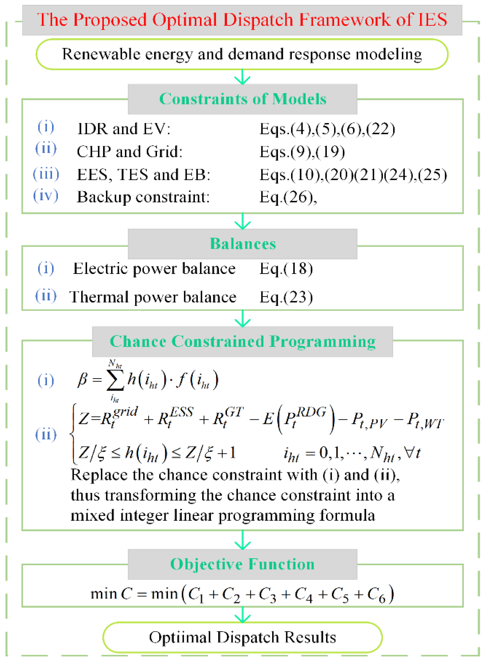
3.3. Solving Process

3.3.1. Sequence Operation Theory

The sequence operation theory is based on sequence convolution in the field of digital signal processing, which extends the original concept of sequence convolution to analyze random variables in the power system. C. Kang et al. [37] proposed the probabilistic sequence operation theory based on the sequence operation theory, which represents the probability distribution of random variables with probabilistic sequences, and then obtains new sequences through the operations between sequences. In this process, through the discretization of the sequence, the merging of the states in the calculation is skillfully realized, and the calculation speed is greatly improved without reducing the calculation accuracy.

The value of each item in the probabilistic sequence is between 0 and 1, representing the occurrence probability of the item. In the proposed IES optimal scheduling model, the DERs are treated as random variables, and their fluctuations follow a certain probability distribution. The probability distribution is discretized to form a probability sequence, and the probability sequence of the equivalent value of all the random variables is obtained through convolution sum and convolution difference operations.

Random variable serialization modeling converts each random variable into a probabilistic sequence according to the requirements of sequence operation theory. If the PDF of a known random variable is F(i), then its probability sequence can be expressed as Equation (27):

$$F\left(i\right)=\left\{\begin{array}{l}{\displaystyle {\int }_{-\infty }^{\Delta p/2}f\left(p\right)dp i=0}\\ {\displaystyle {\int }_{i\Delta p-\Delta p/2}^{i\Delta p+\Delta p/2}f\left(p\right)dp 0<i<N_F}\\ {\displaystyle {\int }_{i\Delta p-\Delta p/2}^{+\infty }f\left(p\right)dp }i=N_F\end{array}\right.$$

(27)

where N_F is the sequence length; N_F = [P_max/Δp] represents an integer no more than P_max/Δp; Δp is the discretization step; P_max is the maximum value of the random variables, indicating the WT and PV output.

3.3.2. Chance-Constrained Programming

In this paper, the probabilistic sequence of the DERs is obtained through convolution summation. According to Equation (27), the probability series of the wind power output and PV output in period t are a(i_at) and b(i_at), with sequence lengths of N_at and N_bt, respectively. The combined output of the DERs is c(i_ct)= a(i_at)⊕b(i_at), with a sequence length of N_ct = N_at + N_bt, which can be calculated by convolution summation, as in Equation (28):

$$c\left(i_{ct}\right)={\displaystyle \sum _{i_{at}+i_{bt}=i_{ct}}a\left(i_{at}\right)·b\left(i_{bt}\right)} , i_{ct}=0,1,\cdots ,N_{ct}$$

(28)

To facilitate the calculation of the spinning-reserve satisfaction probability, the opportunity constraints in Equation (26) need to be handled. The 0–1 variable is defined as Equation (29):

$$h\left(i_{ht}\right)=\left\{\begin{array}{l}1 R_{t1}\ge R_{t2}\\ 0 R_{t1}<R_{t2} \end{array}\right. i_{ht}=0,1,\cdots ,N_{ht}$$

(29)

where R_t1 = ${\mathrm{R}}_t^{\mathrm{grid}}$ + ${\mathrm{R}}_t^{\mathrm{ESS}}$ + ${\mathrm{R}}_t^{\mathrm{GT}}$, R_t2 = E(${\mathrm{P}}_t^{\mathrm{RDG}}$)-P_t,PV-P_t,WT.

The above equation shows that when the IES meets the reserve constraint, the 0–1 variable equals one; otherwise, it equals zero.

The opportunity constraints can be translated into Equation (30):

$$\beta ={\displaystyle \sum _{i_{ht}}^{N_{ht}}h\left(i_{ht}\right)·f\left(i_{ht}\right)}$$

(30)

Once β ≥ α, the spinning reserve satisfies the opportunity constraint. To make (29) compatible with the mixed-integer linear-programming formula, it can be rewritten as Equation (31):

$$\left\{\begin{array}{l}Z=R_t^{\mathrm{grid}}+R_t^{\mathrm{ESS}}+R_t^{\mathrm{GT}}-E\left(P_t^{\mathrm{RDG}}\right)-P_{t,\mathrm{PV}}-P_{t,\mathrm{WT}}\\ Z/\xi \le h\left(i_{ht}\right)\le Z/\xi +1 i_{ht}=0,1,\cdots ,N_{ht},\forall t\end{array}\right.$$

(31)

where ξ is a very large positive number.

Given $R_t^{\mathrm{grid}}$ + $R_t^{\mathrm{ESS}}$ + $R_t^{\mathrm{GT}}$ ≥ E($P_t^{\mathrm{RDG}}$) − P_t,PV − P_t,WT, Equation (31) can be equivalent to ξ ≤ h(i_ht) ≤ ξ + 1, where h(i_ht) is a binary variable (i.e., either 0 or 1). The opportunistic constraint is replaced by Equations (30) and (31), which translate the opportunistic constraint into a mixed-integer linear-programming (MILP) formula.

3.3.3. Solution Steps

The method framework proposed in this paper is shown in Figure 2. The solution process of the system is given as follows:

Figure 2. Framework for optimal scheduling of IES.

Step 1: Establish the IES optimal scheduling model with chance-constrained programming;

Step 2: Discretize the DERs according to their PDFs to generate the corresponding probability sequence;

Step 3: Obtain the expected value of the DER output based on the change in the discretization step size;

Step 4: Convert the probabilistic spinning-reserve constraint into a deterministic constraint;

Step 5: Convert the original chance-constrained-programming-based scheduling model into MILP format;

Step 6: Input the parameters of the IES;

Step 7: Use the CPLEX solver to solve and obtain the optimal solution;

Step 8: Check whether the optimal solution exists. If so, terminate the solution process; otherwise, update the confidence level and repeat the process from Step 6;

Step 9: Output the optimal scheduling scheme.

4. Case Study and Result Analysis

To verify the feasibility of the model and method proposed in this article, this section takes the comprehensive energy system of a smart park as a specific example for simulation analysis.

4.1. Configuration of Case Study

The system structure and its load and DER output profiles are shown in Figure 3 and Figure 4, respectively. Other specific parameters are shown in Table 1.

Figure 3. Topology of the IES used in the case study.

Figure 4. Electricity–heat load demand and DER output.

Table 1. Comprehensive energy system parameters.

Parameter	Value	Parameter	Value
$P_{\max }^{\mathrm{grid}}$	500 kW	CESS,max	160 kW h
P*	500 kW	$P_{\mathrm{HSD},\max }^{\mathrm{CH}}$	60 kW
vci	3 m/s	$P_{\mathrm{HSD},\max }^{\mathrm{DC}}$	60 kW
vco	25 m/s	$P_{\mathrm{t},\max }^{\mathrm{EB}}$	300 kW
v*	15 m/s	ηEB	0.99
PPV,max	360 kW	PEV	900 kW
$C_{t,\mathrm{ESS}}^{\mathrm{START}}$	32 kW h	$P_{k,\mathrm{EV},\max }^{\mathrm{CH}}$	60 kW
CESS,min	32 kW h	$P_{\max }^{\mathrm{GT}}$	500 kW
CESS,max	160 kW h	$P_{\min }^{\mathrm{GT}}$	30 kW
${\eta }_{\mathrm{ESS}}^{\mathrm{CH}}$	0.9	St	1
${\eta }_{\mathrm{ESS}}^{\mathrm{DC}}$	0.9	Ut	1.6
$P_{\mathrm{ESS},\max }^{\mathrm{CH}}$	40 kW	v	1.2
$P_{\mathrm{ESS},\max }^{\mathrm{DC}}$	40 kW	ψ	0.35
$s_{re\_price}^{\mathrm{ESS}}$	CNY 0.02/kWh	κ	1.6
$s_{re\_price}^{\mathrm{grid}}$	CNY 0.06	$s_{dp\_price}^{\mathrm{ESS}}$	CNY 0.02/kW h
$s_{re\_price}^{\mathrm{GT}}$	CNY 0.04	sco2	CNY 0.25/kg

In this paper, the CPLEX solver is used to optimize the solution, and the system is simulated with a cycle of 24 h and a fixed step of one hour. This section compares the operating costs under different scenarios.

Scenario 1: Optimal scheduling of the IES to minimize the overall operation cost of the system without considering the comprehensive demand response or EES/thermal energy storage;

Scenario 2: Optimal scheduling of the IES to minimize the overall operation cost of the system by considering the comprehensive demand response while ignoring the EES and thermal energy storage;

Scenario 3: Optimal scheduling of the IES to minimize the overall operation cost of the system by considering the comprehensive demand response and the optimal scheduling in the IES of the EES and thermal energy storage.

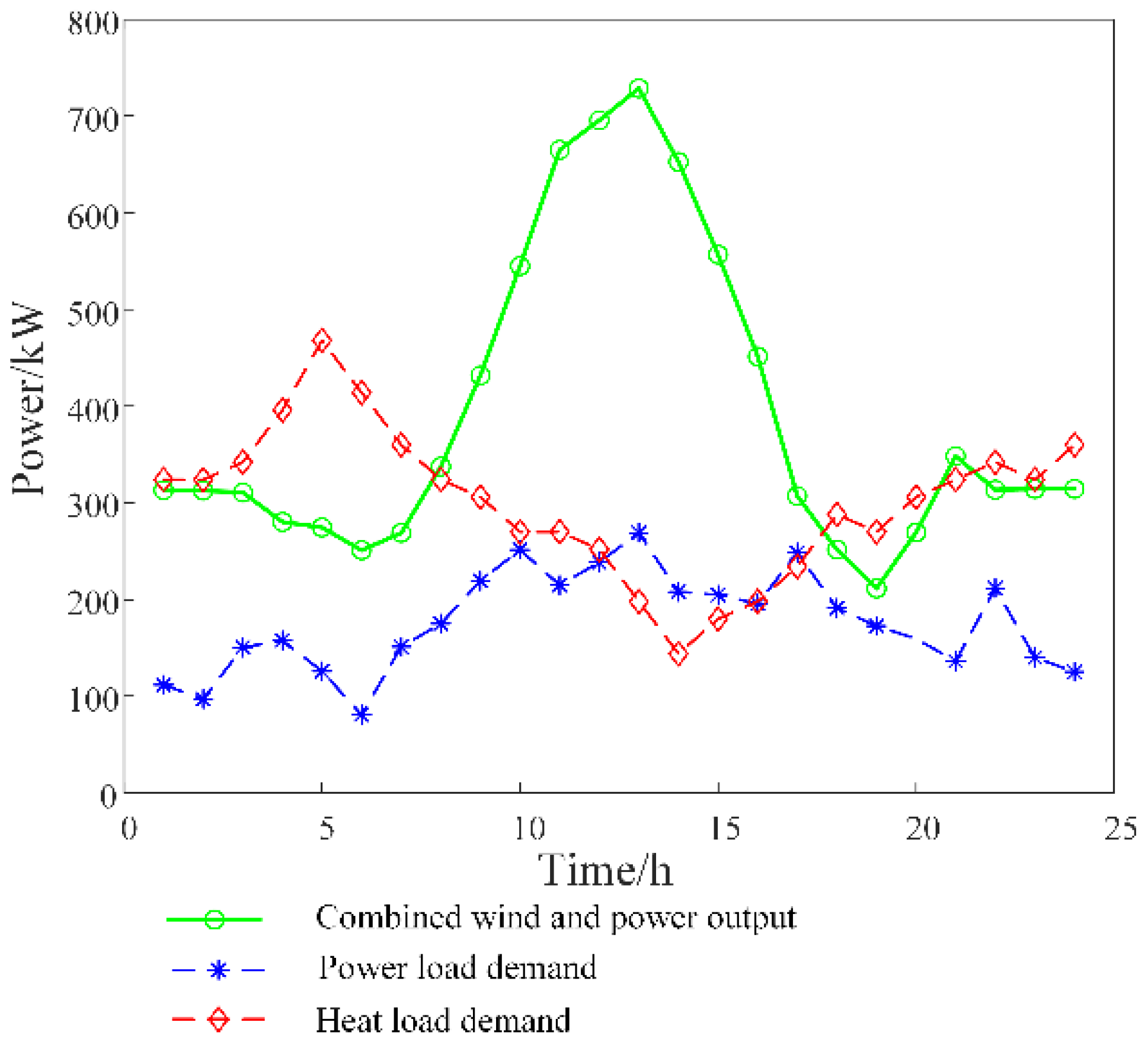
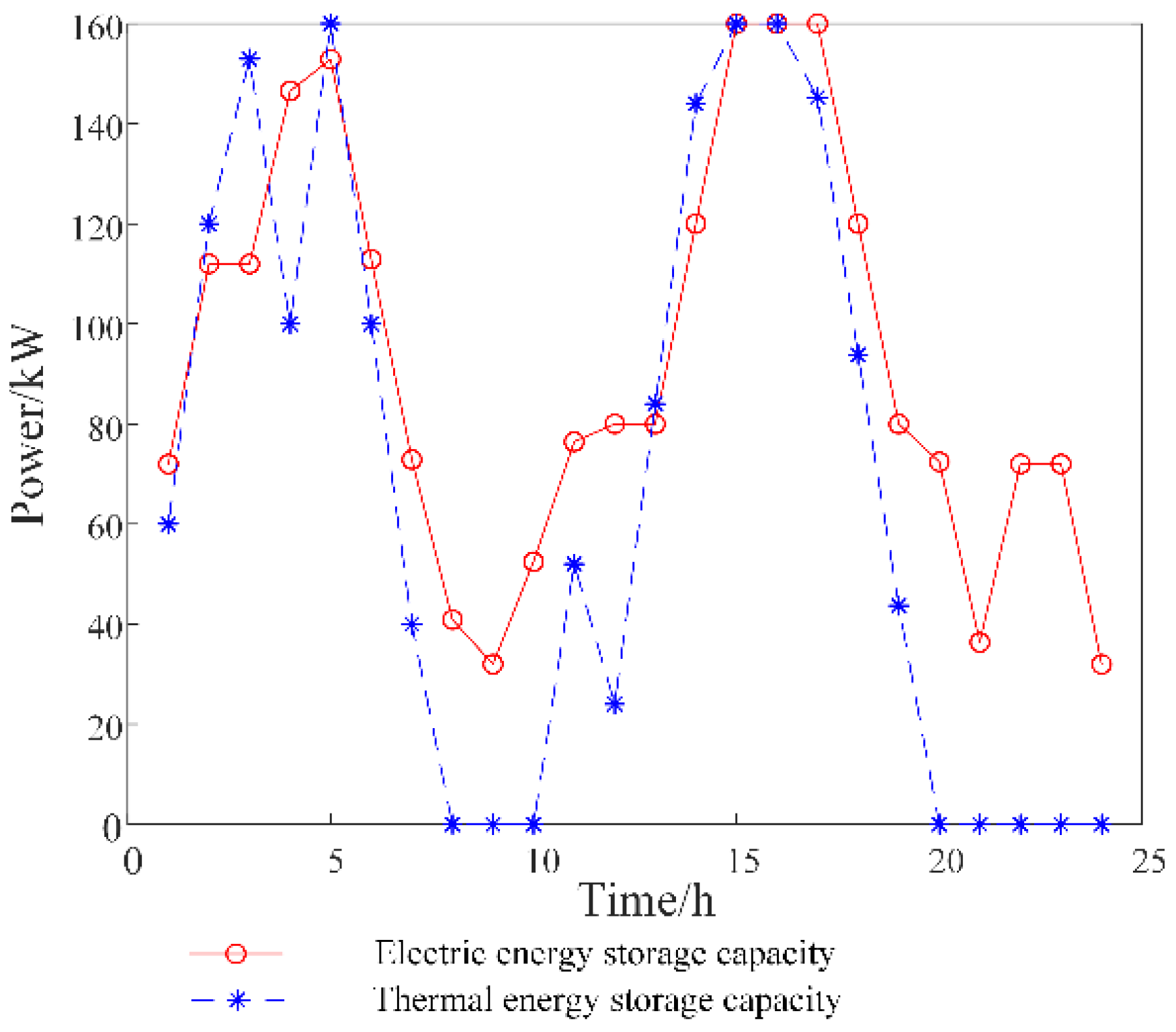
4.2. Discussion of Optimal Scheduling Results

The daily load curve can be divided into three periods: a peak period (8:00–11:00, 18:00–21:00), normal period (6:00–7:00, 12:00–17:00) and valley period (01:00–05:00, 22:00–24:00). The time-of-use prices of the system in this paper are defined as the peak price (CNY 0.805/kWh), normal price (CNY 0.55/kWh) and valley price (CNY 0.295/kWh). The time-of-use load is transferred under the guidance of the time-of-use price, which increases the electricity consumption at the valley time. At the same time, the peak electricity price of the system is high, and the peak load transfer effectively reduces the power consumption cost of the system at the peak time and improves the economy of the system operation.

It can be seen from Table 2 that by comparing the operation cost of the electricity–heat IES before and after considering the price-type demand response, the total operation cost of Scenario 2 is CNY 356.266 (21.01%) lower than that of Scenario 1. The carbon emissions decreased by 291.959 kg, or 46.69%. It is demonstrated that the demand-side response plays an important role in low-carbon economic dispatching, as the demand-side response transfers the peak load to the load valley. Therefore, more economic power can be used in the load valley, and the load power can be reduced in the load peak, thereby reducing the system operation cost.

Table 2. Total costs and carbon emissions under different scenarios.

Parameter	Scenario 1	Scenario 2	Scenario 3
Total cost (CNY)	1695.398	1339.132	1140.278
Carbon emissions (kg)	625.202	333.243	116.013
Carbon transaction cost (CNY)	250.0808	133.2972	46.4052

Compared with Scenario 2, Scenario 3 reduces the total operating cost of the system by 198.854, or 14.85%. The carbon emissions are reduced by 217.23 kg, or 65.15%. This indicates that the addition of EES and thermal energy storage can also effectively reduce the optimal scheduling cost of the system. Figure 5 shows the EES and thermal energy storage scheduling scheme of the system in Scenario 3. It can be seen that the EES and thermal energy storage are charged and stored during the load valley, and then discharged and released during the peak load time. Therefore, the energy consumption of the system can be improved by scheduling the EES and thermal storage equipment, which plays a role in reducing the peak and filling the valley.

Figure 5. Scheduling of EES and thermal energy storage.

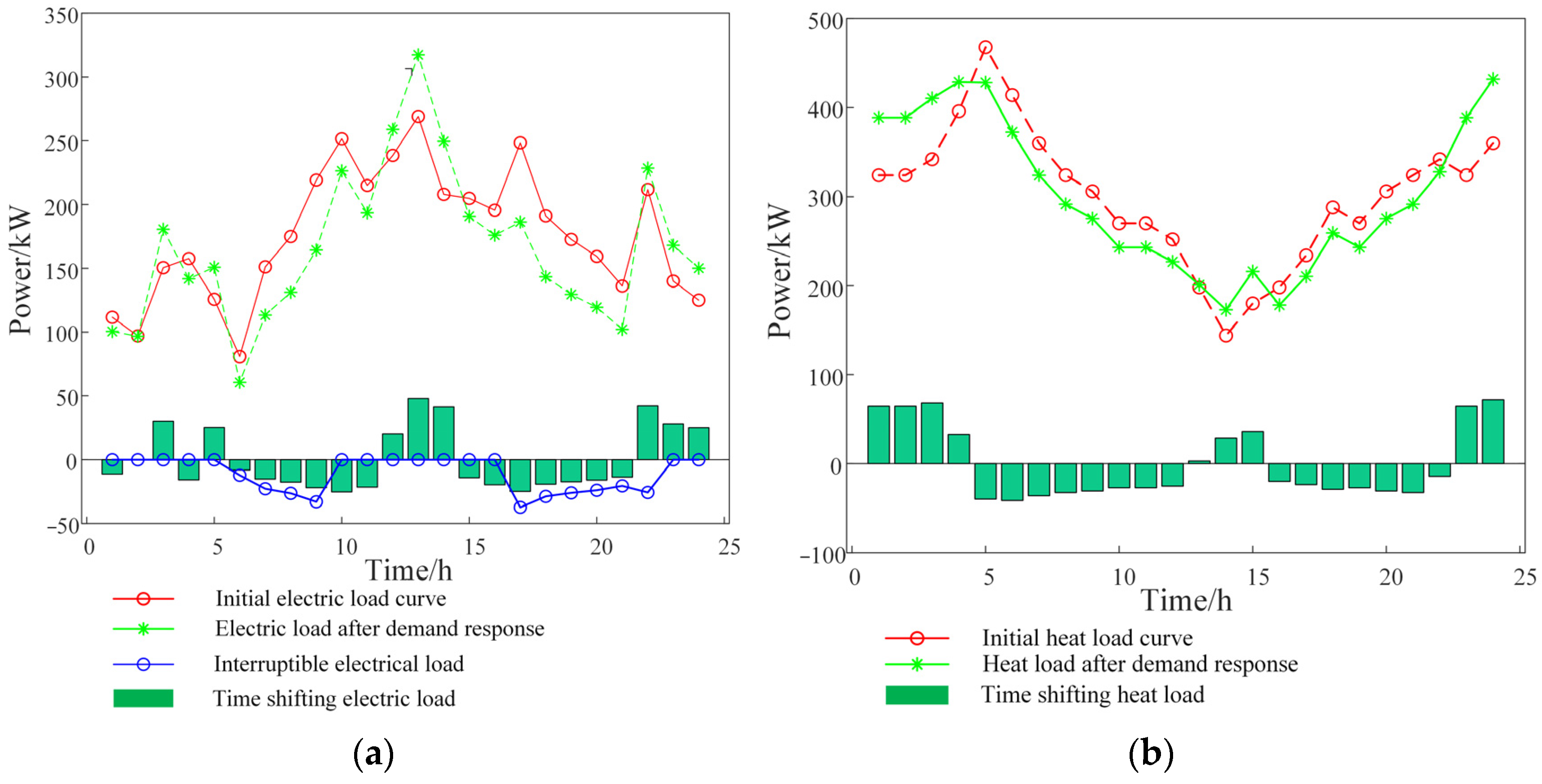
4.3. Demand Response Analysis

4.3.1. Impact of Demand Response Ratio on Economy

For Scenario 3, the impact of the demand response ratio on the overall operating cost of the IES is analyzed. The demand response load of the system available for scheduling is summarized in Table 3.

Table 3. Total system costs under different demand responses.

No.	Parameter	Parameter Values	Operating Cost (CNY)
1	$P_{t,\mathrm{EL}}^{\mathrm{TS}}$ $P_t^{\mathrm{TL}}$ $P_{t,\mathrm{HL}}^{\mathrm{TS}}$	[−0.05 × Pe-load, 0.1 × Pe-load] [0, 0.05Pe-load] [−0.05 × $P_t^{\mathrm{HL}}$, 0.1 × $P_t^{\mathrm{HL}}$]	1313.266
2	$P_{t,\mathrm{EL}}^{\mathrm{TS}}$ $P_t^{\mathrm{TL}}$ $P_{t,\mathrm{HL}}^{\mathrm{TS}}$	[−0.1 × Pe-load, 0.2 × Pe-load] [0, 0.15Pe-load] [−0.1 × $P_t^{\mathrm{HL}}$, 0.2 × $P_t^{\mathrm{HL}}$]	1140.277
3	$P_{t,\mathrm{EL}}^{\mathrm{TS}}$ $P_t^{\mathrm{TL}}$ $P_{t,\mathrm{HL}}^{\mathrm{TS}}$	[−0.2 × Pe-load, 0.4 × Pe-load] [0, 0.35Pe-load] [−0.2 × $P_t^{\mathrm{HL}}$, 0.4 × $P_t^{\mathrm{HL}}$]	860.467

It can be seen from the system operation cost in Table 3 that the overall operation cost of the system decreases with the increase in the demand response load proportion. This is because the demand response can flexibly adjust the load according to the energy consumption of the system, thereby reducing the energy consumption cost of the system. At present, in actual system operations, the proportion of the demand response load available for scheduling is generally between 5 and 30% of the total load, so Case 2 simulates the proportion of the demand response in practical grids. In the future, the energy utilization rate can be effectively improved, and the energy efficiency of the system can be improved by increasing the proportion of the flexible load on the load side.

4.3.2. Demand Response

The load curve before and after the system demand response is analyzed based on the configuration of Case 2. The load curves before and after the comprehensive demand responses in Scenario 3 are shown in Figure 6.

Figure 6. Load curves before and after the comprehensive demand response in Scenario 3. (a) Influence of demand response on electric load. (b) Influence of demand response on heat load.

It can be seen that the load has a certain time shift in each period after the demand response, which improves the energy consumption of the system. In Period 13, the initial power load is at the peak, and the total power load increases after dispatching. The reason is that the overall load demand in the system is small and the electricity price is the normal electricity price, so the loads in the other periods are transferred into this period. In Periods 1–4 and 22–24, the load increases after system dispatching because the system energy consumption is at a low point during this period, and the price of electricity is the lowest. The time-shifting loads can effectively reduce the overall energy consumption cost of the system.

4.4. Influence of Different Confidence Levels

Different confidence levels from 50% to 100% were selected to investigate the impact of the system reserve capacity on the total system operating cost. The corresponding operating costs are calculated and shown in Figure 7. The higher the confidence level, the higher the total operating cost of the system. This is because the increase in the confidence level will inevitably lead to the IES requiring a greater spinning-reserve capacity to maintain the balance between the supply and demand of the system.

Figure 7. System operation costs under different confidence levels.

Figure 8 shows the backup power required by the system at different confidence levels. It is obvious that the higher the confidence level, the more backup capacity required. Therefore, choosing a reasonable confidence level is of great significance to balance the economic benefit and reliability of the system operation. It can be seen that the reserve capacity required by the system changes with time. The peak occurs in Period 13 and the valleys occur in Period 6 and Period 19. The reason is that the DER output in the IES fluctuates over time (as shown in Figure 4). To solve the uncertainty caused by the DER output, it is necessary to set a higher reserve capacity in the period with large DER output and a lower reserve capacity in the period with small DER output.

Figure 8. Reserve capacities at different confidence levels.

Figure 9 shows the reserve capacity of each type of energy when the system confidence level is 90%. It can be seen from Figure 9 that the reserve capacity provided by the energy storage for the system is the least, while the capacity of the gas turbine is more than the energy storage, and that of the power grid is the most. This is mainly because, during the operation of the IES, as the operating cost of energy storage is minimal, the use of the energy storage reserve capacity to power the system is preferred. However, due to the capacity limitation of energy storage itself, the reserve capacity provided by the energy storage is lower than that of the gas turbine and power grid.

Figure 9. System reserve capacity with 90% confidence level.

The reserve capacity of the gas turbine is relatively large, which is mainly because the capacity of the gas turbine is higher than that of the energy storage. The price of the gas turbine for supplying power to the system is CNY 0.35/kWh, which is lower than the price during peak hours and ordinary hours. In addition, the price of the gas turbine reserve capacity is CNY 0.04/kWh, which is lower than the grid reserve price (CNY 0.06/kWh). Therefore, only when the system makes full use of the energy obtained from the gas turbine can the shortfall be obtained from the grid. This is why the reserve provided by the gas turbine is less than that provided by the grid.

The main reason that the grid owns the largest proportion of the reserve capacity is that the price and reserve capacity price of the power grid are higher than those of the energy storage and gas turbines. When the reserve capacity provided by the internal energy storage and gas turbines of the system is insufficient, the power grid will undertake all the demand for the lack of reserve capacity of the whole system.

5. Conclusions

To deal with the uncertainty of the DERs and demand response in the IES, this paper proposes an integrated demand response economic scheduling model based on opportunity-constrained programming to minimize the overall operating cost in an uncertain environment. Through the integrated demand response model, the impact of the demand response ratio on the operating economy of the IES is studied. Based on the case study results, the following conclusions can be drawn:

(1) The proposed IES scheduling model balances the energy demand of the system by coordinating the flexible demand response and the uncertainty of the energy storage equipment and DERs, thereby improving the economy and reducing the carbon emissions of the system;

(2) The operating economy of the IES increases with the increase in the proportion of the demand response. The increase in the flexible load on the demand side of the system not only improves the operating flexibility of the system but also promotes the system’s economic benefit.

In future work, with the continuous increase in new equipment in IESs, it will be necessary to introduce electricity–gas and carbon capture equipment to the IES to promote the regulation of renewable energy production and the complementarity of multiple energy sources, thereby achieving the economic improvement in and energy utilization efficiency of IESs.

References

- Mi, J.; Ma, X. Development trend analysis of carbon capture. utilization and storage technology in china. Proc. CSEE 2019, 39, 2537–2544. [Google Scholar] [CrossRef]
- Ye, K.; Zhao, J.; Zhang, Y.; Liu, X.; Zhang, H. A generalized computationally efficient copula-polynomial chaos framework for probabilistic power flow considering nonlinear correlations of PV injections. Int. J. Electr. Power Energy Syst. 2022, 136, 107727. [Google Scholar] [CrossRef]
- Nastasi, B.; Mazzoni, S. Renewable Hydrogen Energy Communities layouts towards off-grid operation. Energy Convers. Manag. 2023, 291, 117293. [Google Scholar] [CrossRef]
- Fan, J.; Tong, X.; Zhao, J. Multi-period optimal energy flow for electricity-gas integrated systems considering gas inertia and wind power uncertainties. Int. J. Electr. Power Energy Syst. 2020, 123, 106263. [Google Scholar] [CrossRef]
- Li, J.; Ge, S.; Zhang, S.; Xu, Z.; Wang, L.; Wang, C.; Liu, H. A multi-objective stochastic-information gap decision model for soft open points planning considering power fluctuation and growth uncertainty. J. Appl. Energy 2022, 317, 119141. [Google Scholar] [CrossRef]
- Maulik, A. Probabilistic power management of a grid-connected microgrid considering electric vehicles, demand response, smart transformers, and soft open points. Sustain. Energy Grids Netw. 2022, 30, 100636. [Google Scholar] [CrossRef]
- Yang, D.; Wang, M.; Yang, R.; Zheng, Y.; Pandzic, H. Optimal Dispatching of an Energy System with Integrated Compressed Air Energy Storage and Demand Response. Energy 2021, 19, 121232. [Google Scholar] [CrossRef]
- Ge, L.; Li, Y.; Li, Y.; Yan, J.; Sun, Y. Smart Distribution Network Situation Awareness for High-Quality Operation and Maintenance: A Brief Review. Energies 2022, 15, 828. [Google Scholar] [CrossRef]
- Yu, L.; Jiang, T.; Cao, Y.; Qi, Q. Carbon-aware energy cost minimization for distributed internet data centers in smart microgrids. IEEE Internet Things J. 2014, 1, 255–264. [Google Scholar] [CrossRef]
- Han, Z.; Li, Z.; Zhang, W.; Liu, K.; Dong, H.; Yuan, T. Economic operation strategy of hydrogen integrated energy system considering uncertainty of photovoltaic output power. Electr. Power Autom. Equip. 2021, 41, 99–106. [Google Scholar] [CrossRef]
- Zhang, C.; Chen, H.; Liang, Z.; Mo, W.; Zheng, X.; Hua, D. Interval voltage control method for transmission systems considering interval uncertainties of renewable power generation and load demand. IET Gener. Transm. Distrib. 2018, 12, 4016–4025. [Google Scholar] [CrossRef]
- Yi, L.; Hao, S.; Li, G. Towards long-period operational reliability of independent microgrid: A risk-aware energy scheduling and stochastic optimization method. Energy 2022, 254, 124291. [Google Scholar] [CrossRef]
- Guevara, E.; Babonneau, F.; Homem-de-Mello, T.; Moret, S. A machine learning and distributionally robust optimization framework for strategic energy planning under uncertainty. Appl. Energy 2020, 271, 115005. [Google Scholar] [CrossRef]
- Kong, X.; Xiao, J.; Liu, D.; Wu, J.; Wang, C.; Shen, Y. Robust stochastic optimal dispatching method of multi-energy virtual power plant considering multiple uncertainties. Appl. Energy 2020, 279, 115707. [Google Scholar] [CrossRef]
- Wang, C.; Jiao, B.; Guo, L.; Tian, Z.; Niu, J.; Li, S. Robust scheduling of building energy system under uncertainty. Appl. Energy 2016, 167, 366–376. [Google Scholar] [CrossRef]
- Jiang, Y.; Wan, C.; Botterud, A.; Song, Y.; Dong, Z.Y. Efficient robust scheduling of integrated electricity and heat systems: A direct constraint tightening approach. IEEE Trans. Smart Grid 2021, 4, 3016–3029. [Google Scholar] [CrossRef]
- Ma, G.; Lin, Y.; Zhang, Z.; Yin, B.; Pang, N.; Miao, S. A robust economic dispatch method for an integrated energy system considering multiple uncertainties of source and load. Power Syst. Prot. Control. 2021, 49, 43–52. [Google Scholar]
- Zheng, X.; Xu, Y.; Li, Z.; Chen, H. Co-optimisation and settlement of power-gas coupled system in day-ahead market under multiple uncertainties. IET Renew. Power Gener. 2020, 15, 1632–1647. [Google Scholar] [CrossRef]
- Zhao, Z.; Ye, R.; Shu, Z.; Shi, T. Stochastic Dispatch of Regional Integrated Energy System under Multi—Uncertainties. Sci. Technol. Eng. 2021, 21, 4071–4077. [Google Scholar] [CrossRef]
- Cui, Y.; Guo, F.; Zhong, W.; Zhao, Y.; Fu, X. Interval multi-objective optimal dispatch of integrated energy system under multiple uncertainty environment. Power Syst. Technol. 2020, 46, 2964–2975. [Google Scholar] [CrossRef]
- Li, T.; Hu, Z.; Chen, Z.; Liu, S. Multi-time scale low-carbon operation optimization strategy of integrated energy system considering electricity-gas-heat-hydrogen demand response. Electr. Power Autom. Equip. 2021, 43, 16–24. [Google Scholar] [CrossRef]
- Wang, D.; Hu, Q.; Jia, H.; Hou, K.; Du, W.; Chen, N.; Wang, X.; Fan, M. Integrated demand response in district electricity-heating network considering double auction retail energy market based on demand-side energy stations. Appl. Energy 2019, 248, 656–678. [Google Scholar] [CrossRef]
- Huppmann, D.; Egging, R. Market power, fuel substitution and infrastructure—A large-scale equilibrium model of global energy markets. Energy 2014, 75, 483–500. [Google Scholar] [CrossRef]
- Li, P.; Wang, W.; Wei, J.; Li, D.; Long, C.; Chen, W. Optimal operation model of a park integrated energy system considering uncertainty of integrated demand response. Power Syst. Prot. Control. 2022, 50, 163–175. [Google Scholar] [CrossRef]
- Mazzoni, S.; Sze, J.Y.; Nastasi, B.; Ooi, S.; Desideri, U.; Romagnoli, A. A techno-economic assessment on the adoption of latent heat thermal energy storage systems for district cooling optimal dispatch & operations. Appl. Energy 2021, 289, 116646. [Google Scholar] [CrossRef]
- Li, P.; Wu, D.; Li, Y.; Liu, H.; Wang, N.; Zhou, X. Dispatch of multi-microgrids integrated energy system based on integrated demand response and Stackelberg game. Proc. CSEE 2021, 41, 1307–1321+1538. [Google Scholar] [CrossRef]
- Eghbali, N.; Hakimi, S.M.; Hasankhani, A.; Derakhshan, G.; Abdi, B. Stochastic energy management for a renewable energy based microgrid considering battery, hydrogen storage, and demand response. Sustain. Energy Grids Netw. 2022, 30, 100652. [Google Scholar] [CrossRef]
- Godoy, J.; Schierloh, R. Predictive management of the hybrid generation dispatch and the dispatchable demand response in microgrids with heating, ventilation, and air-conditioning (HVAC) systems. Sustain. Energy Grids Netw. 2022, 32, 100857. [Google Scholar] [CrossRef]
- Devine, M.T.; Nolan, S.; MÁ, L.; Mark, O.M. The effect of Demand Response and wind generation on electricity investment and operation. Sustain. Energy Grids Netw. 2019, 17, 100190. [Google Scholar] [CrossRef]
- Guo, W.; Xu, X. Comprehensive energy demand response optimization dispatch method based on carbon trading. Energies 2022, 15, 3128. [Google Scholar] [CrossRef]
- Bossmann, T.; Eser, E.J. Model-based assessment of demand-response measures—A comprehensive literature review. Renew. Sustain. Energy Rev. 2016, 57, 1637–1656. [Google Scholar] [CrossRef]
- Kou, X.; Li, F.; Dong, J.; Olama, M.; Starke, M.; Chen, Y.; Zandi, H. A comprehensive scheduling framework using sp-admm for residential demand response with weather and consumer uncertainties. IEEE Trans. Power Syst. 2021, 36, 3004–3016. [Google Scholar] [CrossRef]
- Yang, C.; Yan, Z.; Zhi, C. Economic analysis of abandoned wind power consumption schemes based on electric-thermal time shift characteristics of regenerative electric boiler. Therm. Power Gener. 2019, 48, 9–17. [Google Scholar] [CrossRef]
- Liu, X. Energy stations and pipe network collaborative planning of integrated energy system based on load complementary characteristics. Sustain. Energy Grids Netw. 2020, 23, 100374. [Google Scholar] [CrossRef]
- Jiang, Y.; Wan, C.; Botterud, A.; Song, Y.; Xia, S. Exploiting flexibility of district heating networks in combined heat and power dispatch. IEEE Trans. Sustain. Energy 2019, 11, 2174–2188. [Google Scholar] [CrossRef]
- Qu, K.; Huang, N.; Yu, T.; Zhang, X. Decentralized dispatch of multi-area integrated energy systems with carbon trading. Proc. CSEE 2018, 38, 697–707. [Google Scholar] [CrossRef]
- Kang, C.; Bai, L.; Xia, Q.; Xiang, N. Probabilistic sequences and operation theory. J. Tsinghua Univ. (Sci. Technol.) 2003, 43, 322–325. [Google Scholar] [CrossRef]
Disclaimer/Publisher’s Note: The statements, opinions and data contained in all publications are solely those of the individual author(s) and contributor(s) and not of MDPI and/or the editor(s). MDPI and/or the editor(s) disclaim responsibility for any injury to people or property resulting from any ideas, methods, instructions or products referred to in the content. |
© 2024 by the authors. Licensee MDPI, Basel, Switzerland. This article is an open access article distributed under the terms and conditions of the Creative Commons Attribution (CC BY) license (https://creativecommons.org/licenses/by/4.0/).