A Comparative Study of Fuel Density Precision Data Using Digital Densimeter Meters at Two Different Temperatures

Abstract

The widespread use of liquid fuels can be monitored by their density and light fractions, which affect storage, combustion, handling, and contractual issues. The quantitative measurement of fuel density is carried out using an analytical procedure whose test method presents precision data (repeatability and reproducibility) at 15 °C, whereas Brazilian commercial legislation uses a base temperature of 20 °C. Therefore, the scope of this study was to evaluate whether there are statistically significant differences between these two temperatures. An interlaboratory study, considering homogeneity and stability checks, was carried out, and the data were treated using a one-way analysis of variance in a single-stage nested design for calculating the density precision data (under repeatability and reproducibility conditions). After using an F test to compare the variances at 15 °C and 20 °C, one concluded that these precision data are not always metrologically comparable.

1. Introduction

Density is an essential physicochemical property, which, when used connected with other properties to characterize the heavy and light fractions in oil and gas, acts as a quality indicator for automobile, aviation, and marine fuels, as it can affect storage, handling, and combustion [1,2,3,4,5].

The most common way of determining density in industry and research is by using digital densimeters, such as in biotechnological processes [6], vegetable oils [7], drugs [8], and fossil fuels [9,10,11]; overviews of the issues regarding measuring and calculating crude oil density can be found in [12,13,14].

Determining of the density of petroleum and its derivatives is necessary to convert the measured volumes to volumes at standard temperature, which in Brazil is 20 °C. However, to comply with international regulations, the precision data, under conditions of repeatability and reproducibility (r&R) of the test method obtained by statistical evaluation of the results of interlaboratory tests are carried out at a test temperature of 15 °C.

Precision data are an important and very useful parameter for evaluating metrological properties in different areas, such as the characterization of certified reference material [15], validation of methods for heavy metal detection [16], detection of honey adulteration [17], the determination of carotenoids in fish and poultry feed [18], and uncertainty evaluation [19].

The quantitative measurement of fuel density is carried out using an analytical procedure based on the ASTM test method that considers the temperature for precision data as being 15 °C, which does not represent Brazilian commercial legislation.

Therefore, this study aimed to statically compare the precision data in terms of repeatability and reproducibility of density using digital densimeter meters [1] at temperatures of 15 °C and 20 °C via interlaboratory tests connected to the F test to decide whether there is metrological comparability between these precision data at these different temperatures or not. In other words, can the repeatability and reproducibility data reported in the ASTM test method at 15 °C be used when this physicochemical property is measured at 20 °C?

A user-friendly spreadsheet based on these metrological assumptions is available to assist users with calculations.

2. Methodology

An interlaboratory test can be defined as the assessment of measurements or tests on the same or similar objects by two or more laboratories vis-à-vis pre-established conditions. This powerful tool is very effective in clarifying some issues in the oil and gas industry, such as evaluating the mechanical properties of gas pipelines [20] and whether there are systematic errors between different test methods for determining the mass fraction of sulfur in gasoline [21].

The supplier/organizer of interlaboratory studies (ILS) must ensure that batches of interlaboratory study items are sufficiently homogeneous and stable for their purpose through criteria that ensure that these parameters do not adversely affect the performance assessment [22].

2.1. Assessment of the Homogeneity of the Items in the Interlaboratory Study

Homogeneity is a critical requirement, including aspects within and between participants. Homogeneity between participants is vital to ensure that each participant has the same value for each property; it also ensures that each subsample represents the same quality characteristic within a laboratory.

The estimate of the standard deviation within the sample bottles, s_w, and the standard deviation between bottles of the same sample, s_s, can be calculated using the analysis of variance, as described below for t bottles of the same sample analyzed in duplicate.

The detailed algorithms for this evaluation follow ISO 13528 [22] and ISO 5725-2 [23], Equations (1)–(8).

$${\overline{x}}_t=\left(x_{t,1}+x_{t,2}\right)/2$$

(1)

$$w_t=\left|x_{t,1}-x_{t,2}\right|$$

(2)

$$\overline{x}=\frac{1}{g}{\sum }_{t=1}^g{\overline{x}}_t$$

(3)

$$s_{\overline{x}}=\sqrt{{\sum }_{t=1}^g{\left({\overline{x}}_t-\overline{x}\right)}^2/\left(g-1\right)}$$

(4)

$$s_w=\sqrt{{\sum }_{t=1}^g{w}_t^2/\left(2g\right)}$$

(5)

$$s_s=\sqrt{\mathrm{maximum}\left(0,s_{\overline{x}}^2-s_w^2/2\right)}$$

(6)

$${\sigma }_{pt}=\sqrt{{\sigma }_R^2-{\sigma }_r^2\left(1-1/m\right)}$$

(7)

Finally, the standard deviation between bottles of the same sample, $s_s$, (Equation (6)) is compared with the standard deviation for evaluating proficiency during an interlaboratory study, ${\sigma }_{pt}$, (Equation (7)). The items of the interlaboratory study can be considered adequately homogeneous if [22]:

$$s_s\le 0.3\times {\sigma }_{pt}$$

(8)

where ${\overline{x}}_t$ and $w_t$ are the sample bottle means and amplitudes, respectively, in each sample bottle; $\overline{x}$ is the overall average; g is the total number of sample bottles; $s_{\overline{x}}$ and s_w are the standard deviation of the sample means and the standard deviation within the sample bottles, respectively; $s_s$ is the standard deviation between bottles of the same sample; ${\sigma }_{pt}$ is the robust standard deviation for evaluation calculated for an interlaboratory study; and m is the number of replicates that each participant must perform in one round of the interlaboratory study.

These estimates can be calculated using the analysis of variance as described below for t bottles of the same sample analyzed in duplicate.

2.2. Assessment of the Stability of Interlaboratory Study Items

In an interlaboratory study, the participant samples must be sufficiently stable for the intended use so that the end user can trust the assigned value at any time within the study period. Typically, it is essential to consider stability under long-term storage conditions, shipping conditions, and, when applicable, storage conditions in the participating user’s laboratory. This procedure may include consideration of stability after opening if reuse is permitted.

A procedure for a basic stability check using measurements before and after a run of an interlaboratory study is based on reference [22].

Compare the grand mean of the measurements obtained in the verification before distribution, here named ${\overline{y}}_1$ and calculated using Equation (3), with the grand mean of the results obtained in the stability verification, ${\overline{y}}_2$. Interlaboratory study test sample bottles may be considered adequately stable if [22]:

$$\left|{\overline{y}}_1-{\overline{y}}_2\right|\le 0.3\times {\sigma }_{pt}$$

(9)

2.3. Using Analysis of Variance (ANOVA) for Data from an Interlaboratory Study

In simple terms, ANOVA determines whether different “treatments” have a statistically significant effect on the mean value. In an ANOVA, the variance of individual test determinations from the overall mean is divided into different sources of variance. One source is “treatments” and the other is “random error”. In the case of data from an interlaboratory study, the source “treatment” corresponds to the “between laboratory” variation component and “random error” corresponds to single-operator variation.

One-way ANOVA is so called because the effect of only one factor, in this case the “laboratory”, is being examined.

For h samples and n replicates, $N=nh$, $T_i$ is the sum of the measurements for the ith sample and $T$ is the total sum of the measurements. The algorithms are presented in

Table 1. Algorithms for one-way ANOVA.

Source of Variation	Sum of Squares (SS)	Degrees of Freedom (ν)	Mean Squares (MS)	Fcalculated
Between samples (A)	${\displaystyle \sum _i}{T}_i^2/n-T^2/N$	$h-1$	$S{S}_A/{\nu }_A$	$M{S}_A/M{S}_r$
Within samples (residual, r)	by subtraction	by subtraction	$S{S}_r/{\nu }_B$
Total	${\displaystyle \sum _i}{\displaystyle \sum _j}{x}_{ij}^2-T^2/N$	$N-1$

[24].

The column labeled “SS” represents the “sum of squares or quadratic sum”, and the column labeled “MS” represents the “mean of squares or quadratic mean”. Mean squares are calculated by dividing the quadratic sum by their respective degrees of freedom.

The combined single-operator variance is equal to the mean squared residual or error. Therefore, repeatability can be estimated as $\sqrt{{MS}_r}$ [25].

The quadratic mean between laboratories, ${MS}_L$, is related to the component of variances between laboratories: ${MS}_L=n{s}_L^2+{MS}_r$ [25].

Thus, the between-laboratory variance component $s_L^2$ is $\frac{{MS}_L-{MS}_r}{n}$ for $n$ replicates. Finally, reproducibility can be estimated as $\sqrt{\frac{{MS}_L-{MS}_r}{n}}$. If ${MQ}_L$ is less than ${MS}_r$, the between-laboratory variance component is set equal to zero [25].

2.4. F Test for Comparing Variances

In many cases, it is important to compare the standard deviations or variances, that is, the random errors of two data sets. The test $F$ considers the ratio of the two sample variances, that is, the ratio of the squares of the standard deviations, $s_1^2/s_2^2$.

When one wants to test whether there is a significant difference between two sample variations, that is, to test $H_0:{\sigma }_1^2/{\sigma }_2^2$, the statistic $F$ is calculated: $F=s_1^2/s_2^2$, where the subscripts 1 and 2 are considered in the equation so that F is always ≥1. The number of freedom degrees of the numerator and the denominator are, respectively, $n_1-1$ and $n_2-1$. The test considers that the populations from which the samples obtained follow a normal distribution.

The probability of the $F$ test was calculated using MS Excel via the function “dist.F” (value; degrees of freedom 1; degrees of freedom 2; TRUE), Table 1. The cumulative argument “TRUE” considers the probability of $F$ using the cumulative distribution function. The “value” argument is the ratio between the variances, so that the ratio between them is always ≥1 [26].

3. Experimental

Based on the reality of the Brazilian energy matrix, the interlaboratory study regarding samples of S10 diesel oil, biodiesel (B100), and VLSFO (very low sulfur fuel oil) or bunker (

Table 2. Study profile.

Fuel	Property	Test Method
S10 diesel oil	Density	ASTM D4052-22
Biodiesel (B100)
VLSFO

) was carried out from May to August 2022. All measuring equipment used was calibrated and within its expiration date.

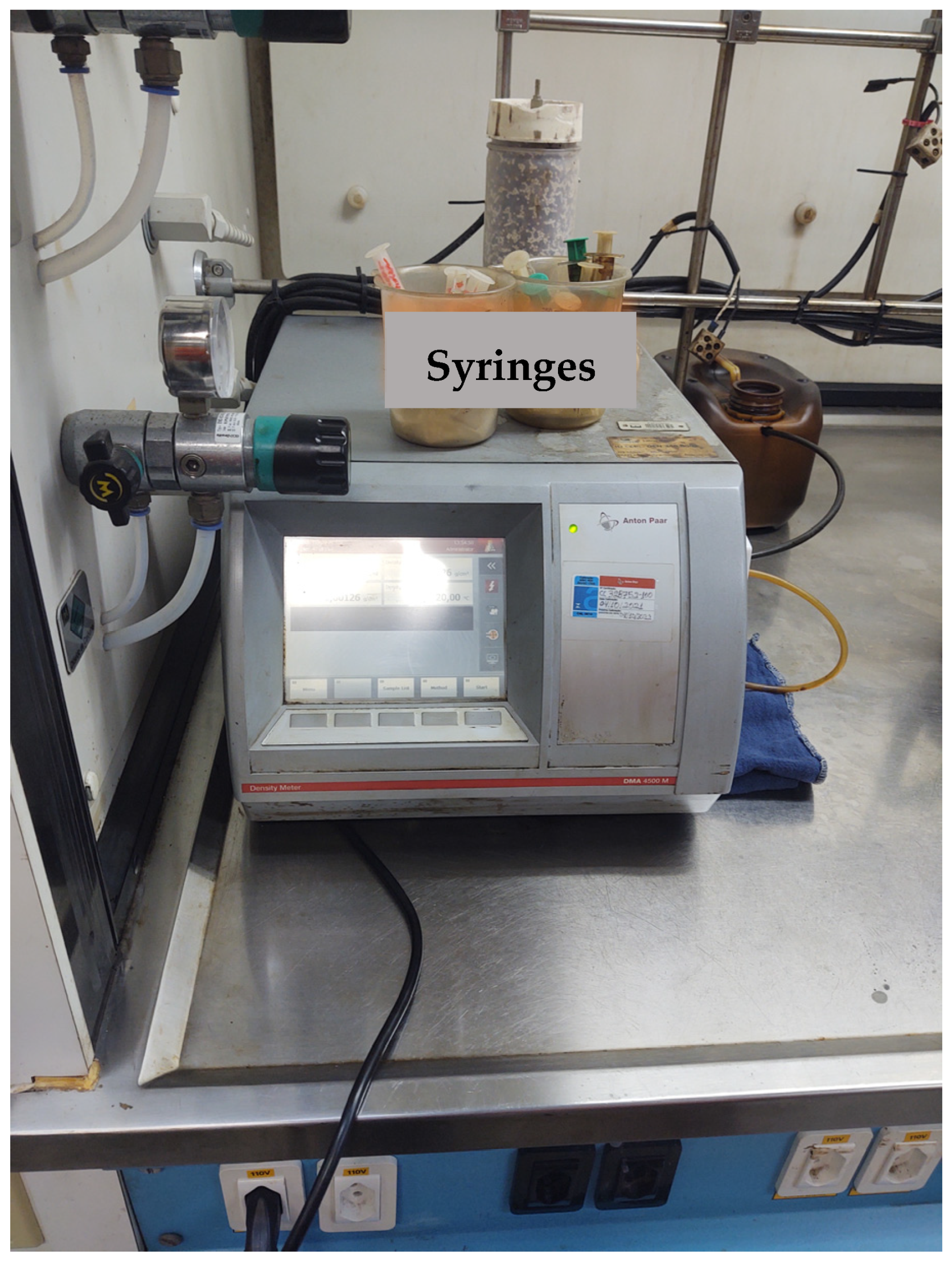
A volume of roughly 1 mL to 2 mL of liquid sample was introduced into an oscillating U-tube using a suitable syringe for manual injections. The oscillation frequency variation caused by the change in mass of the U-tube was used in conjunction with the calibration data to determine the density of the sample [1], Figure 1.

Sample volumes of 750 mL were collected in bottles with a capacity of 1 L and sealed with a lid and stopper.

Seven laboratories participated in the interlaboratory study. Except for laboratory 6, all laboratories used Anton Parr equipment; however, laboratory 2 participated with three different equipment models,

Table 3. Participating laboratories and their equipment models used.

Laboratory	Equipment Model
1	DMA 4500M
2	DMA 4500M, DMA 4500, and DMA 48
3	DMA 4500M
4	DMA 4500A
5	DMA 4500M
6	Kyoto DA500
7	MODEL D5

.

In this study, five replicates per sample were analyzed at 15 °C and 20 °C.

Laboratory 6 was responsible for the homogeneity and stability tests of the S10 diesel and biodiesel samples, and laboratory 4 was responsible for the homogeneity and stability tests of the VLSFO samples of this analytical correlation study.

3.1. Homogeneity Test

The homogeneity test was carried out, and the density of the ten vials of each sample was determined in duplicate. For this step, an aliquot from each bottle was taken, selecting the bottle at random and analyzing the density at 20/4 °C. Then, a new aliquot was taken and the experiment was carried out again, selecting the vial randomly.

In total, the experiment collected 58 densities (29 pairs), 10 densities of S10 diesel and biodiesel and nine densities of VLSFO.

3.2. Stability Test

This test was carried out after all laboratories had completed the tests.

To do this, an aliquot from each bottle was taken, selecting the bottle at random and analyzing the density at 20/4 °C. Then, a new aliquot was taken and the experiment was carried out again, selecting the vial randomly. In total, two densities (3 pairs) were determined per product.

4. Results and Discussion

The data were processed based on ISO 13528:2022 [22] to evaluate the homogeneity and stability of the samples and by ASTM C802-14(2022) [25] to calculate repeatability and reproducibility. An Excel spreadsheet was provided with this manuscript as Supplementary Material to manually enter and evaluate data homogeneity, stability, repeatability, and reproducibility, as well as compare variances. The editable cells, with the input data, are on a sky-blue background.

The robust standard deviation evaluated during the interlaboratory study (Equation (7)) was calculated from repeatability (σ_r) and reproducibility (σ_R) standard deviations from previous collaborative studies. For the homogeneity and stability tests, in which the relative density, D, was the parameter evaluated, such inputs come from ASTM D4052:2022 [1].

4.1. Homogeneity Test

The sample from each bottle was analyzed for the density quality characteristic in duplicate, and the data were treated using Equations (1)–(8),

Table 4. Density results for the homogeneity test (g cm⁻³).

	Diesel S10		Biodiesel		VLSFO
Bottle	Replicate 1	Replicate 2	Replicate 1	Replicate 2	Replicate 1	Replicate 2
1	0.8325	0.8326	0.8797	0.8798	0.9308	0.9308
2	0.8326	0.8326	0.8798	0.8798	0.9308	0.9308
3	0.8326	0.8326	0.8798	0.8798	0.9308	0.9307
4	0.8326	0.8326	0.8798	0.8798	0.9307	0.9308
5	0.8326	0.8326	0.8798	0.8798	0.9308	0.9306
6	0.8326	0.8326	0.8798	0.8798	0.9307	0.9308
7	0.8326	0.8326	0.8798	0.8798	0.9308	0.9308
8	0.8326	0.8326	0.8798	0.8798	0.9308	0.9308
9	0.8326	0.8326	0.8798	0.8798	0.9308	0.9307
10	0.8326	0.8326	0.8798	0.8799
$\overline{x}={\overline{y}}_1$	0.832595		0.8799		0.9308
$s_{\overline{x}}$	0.000016		0.000024		0.000035
$s_w$	0.000022		0.000032		0.000067
$s_s$	0.000000		0.000007		0.000000
${\sigma }_{pt}$	0.00051		0.00051		0.00051
$0.3\times {\sigma }_{pt}$	0.00015		0.00015		0.00015
Situation	homogeneous		homogeneous		homogeneous

.

${\sigma }_{pt}=\sqrt{{\sigma }_R^2-{\sigma }_r^2\left(1-1/m\right)}=\sqrt{{0.00052}^2-{0.00016}^2\times \left(1-1/2\right)}=0.00051\mathrm{g}{\mathrm{c}\mathrm{m}}^{-3}$ and the $0.3\times {\sigma }_{pt}=$ $0.00015\mathrm{g}{\mathrm{c}\mathrm{m}}^{-3}.$

Homogeneity was checked in all bottles and in the three products, whereas those $s_s$ values (Table 4) $\le 0.00015\mathrm{g}{\mathrm{c}\mathrm{m}}^{-3}$.

4.2. Stability Test

After all laboratories carried out the tests, the sample from each bottle was analyzed for the density quality characteristic in duplicate and the data were treated using Equation (9),

Table 5. Density results for the stability test (g cm⁻³).

	Diesel S10		Biodiesel		VLSFO
Bottle	Replicate 1	Replicate 2	Replicate 1	Replicate 2	Replicate 1	Replicate 2
1	0.8325	0.8326	0.8799	0.8800	0.9308	0.9307
${\overline{y}}_1$	0.83260		0.87980		0.93077
${\overline{y}}_2$	0.83255		0.87995		0.93075
$\left|{\overline{y}}_1-{\overline{y}}_2\right|$	0.000045		0.000150		0.00017
$0.3\times {\sigma }_{pt}$	0.000152		0.000152		0.000152
Situation	stable		stable		stable

.

${\sigma }_{pt}=\sqrt{{\mathsf{\sigma }}_{\mathrm{R}}^2-{\mathsf{\sigma }}_{\mathrm{r}}^2\left(1-1/\mathrm{m}\right)}=\sqrt{{0.00052}^2-{0.00016}^2\times \left(1-1/2\right)}=0.00051\mathrm{g}{\mathrm{c}\mathrm{m}}^{-3}.$ It is $0.3\times {\sigma }_{pt}=$ $0.00015\mathrm{g}{\mathrm{c}\mathrm{m}}^{-3}.$

Stability was checked in all bottles and the three products since the $\left|{\overline{y}}_1-{\overline{y}}_2\right|$ (Table 5) $\le 0.00015\mathrm{g}{\mathrm{c}\mathrm{m}}^{-3}$.

4.3. Calculation of Repeatability and Reproducibility

The results of the five replicates are found in

Table 6. S10 diesel oil results (k gm⁻³).

	Laboratory/Model	1st	2nd	3rd	4th	5th
20 °C	Lab 1/DMA 4500	832.60	832.60	832.60	832.60	832.70
	Lab 2/DMA 48	832.50	832.50	832.60	832.60	832.60
	Lab 2/DMA 4500	832.61	832.64	832.64	832.69	832.59
	Lab 2/DMA 4500M	832.49	832.51	832.52	832.50	832.51
	Lab 3/4500M	832.64	832.60	832.64	832.60	832.60
	Lab 4/4500A	832.50	832.50	832.50	832.50	832.50
	Lab 5/4500M	833.00	833.00	833.10	833.00	833.10
	Lab 6/Kyoto DA500	832.70	832.70	832.90	832.90	832.90
	Lab 7/MODEL D5	832.50	832.60	832.60	832.60	832.60
15 °C	Lab 1/DMA 4500	836.90	836.80	836.90	837.00	836.60
	Lab 2/DMA 48	836.40	836.40	836.30	836.30	836.30
	Lab 2/DMA 4500	836.20	836.18	836.20	836.22	836.25
	Lab 2/DMA 4500M	836.15	836.19	836.11	836.20	836.16
	Lab 3/4500M	836.17	836.18	836.18	836.18	836.18
	Lab 4/4500A	836.00	836.00	836.00	836.00	836.00
	Lab 5/4500M	836.00	836.10	835.90	836.00	836.10
	Lab 6/Kyoto DA500	837.20	837.20	837.20	837.20	837.20
	Lab 7/MODEL D5	836.00	836.00	835.90	836.00	836.00

and

Table 7. ANOVA results for diesel oil S10 (k gm⁻³).

Source of Variation	MS (20 °C)	MS (15 °C)
Between groups (L)	0.149671	0.881344
Within groups (r)	0.002671	0.00411

(S10 diesel oil),

Table 8. Biodiesel results (k gm⁻³).

	Laboratory/Model	1st	2nd	3rd	4th	5th
20 °C	Lab 1/DMA 4500	879.90	879.80	879.90	879.90	879.80
	Lab 2/DMA 48	879.90	879.90	879.90	879.80	879.80
	Lab 2/DMA 4500	879.98	880.02	880.01	880.00	880.02
	Lab 2/DMA 4500M	879.84	879.85	879.86	879.91	879.91
	Lab 3/4500M	880.01	880.01	880.01	880.01	880.01
	Lab 4/4500A	879.80	879.80	879.80	879.80	879.80
	Lab 5/4500M	879.70	879.80	879.80	879.70	879.60
	Lab 6/Kyoto DA500	879.90	879.90	879.90	879.90	879.90
	Lab 7/MODEL D5	879.80	879.80	879.80	879.80	879.80
15 °C	Lab 1/DMA 4500	883.80	883.80	884.00	883.80	883.80
	Lab 2/DMA 48	883.40	883.30	883.30	883.20	883.20
	Lab 2/DMA 4500	883.60	883.61	883.61	883.62	883.63
	Lab 2/DMA 4500M	883.51	883.58	883.60	883.52	883.43
	Lab 3/4500M	883.68	883.68	883.67	883.67	883.67
	Lab 4/4500A	883.50	883.50	883.50	883.50	883.50
	Lab 5/4500M	882.80	882.80	883.00	882.80	882.90
	Lab 6/Kyoto DA500	883.60	883.60	883.60	883.60	883.60
	Lab 7/MODEL D5	883.40	883.30	883.30	883.30	883.30

and

Table 9. ANOVA results for biodiesel (k gm⁻³).

Source of Variation	MS (20 °C)	MS (15 °C)
Between groups (L)	0.044695	0.406933889
Within groups (r)	0.001601111	0.003292222

(biodiesel), and

Table 10. VLSFO results (k gm⁻³).

	Laboratory/Model	1st	2nd	3rd	4th	5th
20 °C	Lab 4/DMA 4500 A	930.60	930.80	930.60	930.60	930.60
	Lab 7/MODEL D5	932.04	932.04	932.03	932.03	932.03
	Lab 3/4500M	930.80	930.80	930.80	930.90	930.80
	Lab 5/4500M	931.00	930.90	930.90	930.80	931.00
	Lab 1/DMA 4500	930.30	930.40	930.50	930.50	930.50
	Lab 6/Kyoto DA500	932.00	932.00	932.00	932.00	932.00
15 °C	Lab 4/DMA 4500 A	934.70	934.90	934.80	934.90	934.90
	Lab 7/MODEL D5	935.90	935.89	935.85	935.81	935.99
	Lab 3/4500M	934.80	934.80	934.80	934.90	934.80
	Lab 5/4500M	934.90	935.00	934.80	934.90	935.00
	Lab 1/DMA 4500	934.80	934.90	934.90	934.90	934.90
	Lab 6/Kyoto DA500	935.20	934.80	935.40	935.40	935.60

and

Table 11. ANOVA results for VLSFO (k gm⁻³).

Source of Variation	MS (20 °C)	MS (15 °C)
Between groups (L)	2.028978095	0.787493333
Within groups (r)	0.006004286	0.016788571

(VLSFO); to calculate the repeatability and reproducibility of the test method per product at 15 °C and 20 °C, the ANOVA test was applied to these data sets.

A factor of 1000 was used to convert the results from k gm⁻³ to g cm⁻³.

The repeatability can be estimated as $\sqrt{{MS}_r}$ = 0.000052 g cm⁻³ and 0.000064 g cm⁻³, respectively, for 20 °C and 15 °C.

Then, the reproducibility can be estimated as $\sqrt{\frac{{MS}_L-{MS}_r}{n}}$ = 0.000171 g cm⁻³ and 0.000419 g cm⁻³, respectively, for 20 °C and 15 °C.

The repeatability can be estimated as $\sqrt{{MS}_r}$ = 0.000040 g cm⁻³ and 0.000057 g cm⁻³, respectively, for 20 °C and 15 °C.

Then, the reproducibility can be estimated as $\sqrt{\frac{{MS}_L-{MS}_r}{n}}$ = 0.000093 g cm⁻³ and 0.000284 g cm⁻³, respectively, for 20 °C and 15 °C.

The repeatability can be estimated as $\sqrt{{MS}_r}$ = 0.000077 g cm⁻³ and 0.000130 g cm⁻³, respectively, for 20 °C and 15 °C.

Then, the reproducibility can be estimated as $\sqrt{\frac{{MS}_L-{MS}_r}{n}}$ = 0.000636 g cm⁻³ and 0.000393 g cm⁻³, respectively, for 20 °C and 15 °C.

4.4. F Test for Comparing Variances

For S10 diesel and biodiesel, 36 and 8 degrees of freedom were considered, respectively, for repeatability and reproducibility; however, for VLSFO, 28 and 6 degrees of freedom were considered, respectively, for repeatability and reproducibility (

Table 12. F test and probabilities.

Fuel	Repeatability g cm−3		Probability Fcalculated	Reproducibility g cm−3		Probability Fcalculated
	15 °C	20 °C		15 °C	20 °C
Diesel S10	0.000064	0.000052	0.900	0.000419	0.000171	0.990
Biodiesel	0.000040	0.000093	0.983	0.000057	0.000284	0.998
VLSFO	0.000130	0.000077	0.996	0.000393	0.000636	0.867

).

For a significance level of 0.05, there is no metrological comparability of the density at 15 °C and 20 °C for precision in terms of the repeatability for biodiesel and VLSFO, as the values are above 0.95. On the other hand, there is no metrological comparability of the density at 15 °C and 20 °C for precision in terms of reproducibility for S10 diesel oil and biodiesel, as the values are above 0.95.

5. Conclusions

This study statically compared the density precision data measured by digital densimeter meters at temperatures of 15 °C and 20 °C using an interlaboratory comparison methodology. Subsequently, the F test was used to evaluate if there was metrological comparability between the repeatability and reproducibility data at these different temperatures. A customized spreadsheet, available as Supplementary Material, assessed the homogeneity, stability, and precision of the data, in addition to comparing variances. Ultimately, this tool can help users decide on metrological compatibility.

From the results and discussion presented in this study, it can be concluded that the metrological comparability of precision data in terms of the repeatability and reproducibility of density measurements using digital densimeters at temperatures of 15 °C and 20 °C is not always guaranteed, i.e., the repeatability and reproducibility data reported in the ASTM test method at 15 °C cannot be used as if this physicochemical property was measured at 20 °C. Therefore, this study recommends that precision data (repeatability and reproducibility) for the density of liquid fossil fuels by digital density meters be calculated based on local commercial legislation rather than using those presented by ASTM D4052, which are only reported at 15 °C. The methodology developed in this study is very useful, not only for evaluating density precision data but for any other physicochemical property.

As future work that is also relevant in oil operations, we propose to consider as advice the problems of high numbers of errors in density determinations associated with incompatibility and loss of stability in ships’ residual heating oil. Due to the violation of colloidal stability in fuels, changes occur at the molecular level that alter the physicochemical properties, including the density index.

References

- ASTM D4052-22; Standard Test Method for Density, Relative Density, and API Gravity of Liquids by Digital Density Meter. ASTM International: West Conshohocken, PA, USA, 2022. [CrossRef]
- Efimov, I.; Smyshlyaeva, K.I.; Povarov, V.G.; Buzyreva, E.D.; Zhitkov, N.V.; Vovk, M.A.; Rudko, V.A. UNIFAC residual marine fuels stability prediction from NMR and elemental analysis of SARA components. Fuel 2023, 352, 129014. [Google Scholar] [CrossRef]
- Kondrasheva, N.K.; Kondrashev, D.O.; Rudko, V.A.; Shaidulina, A.A. Effect of Hydrocarbon Composition on Quality and Operating Characteristics of Middle Distillate Fractions and Low-Viscosity Marine Fuels. Chem. Technol. Fuels Oils 2017, 53, 163–172. [Google Scholar] [CrossRef]
- Kondrasheva, N.K.; Rudko, V.A.; Kondrashev, D.O.; Gabdulkhakov, R.R.; Derkunskii, I.O.; Konoplin, R.R. Effect of Delayed Coking Pressure on the Yield and Quality of Middle and Heavy Distillates Used as Components of Environmentally Friendly Marine Fuels. Energy Fuels 2019, 33, 636–644. [Google Scholar] [CrossRef]
- Nelyubov, D.V.; Fakhrutdinov, M.I.; Sarkisyan, A.A.; Sharin, E.A.; Ershov, M.A.; Makhova, U.A.; Makhmudova, A.E.; Klimov, N.A.; Rogova, M.Y.; Savelenko, V.D.; et al. New Prospects of Waste Involvement in Marine Fuel Oil: Evolution of Composition and Requirements for Fuel with Sulfur Content up to 0.5%. J. Mar. Sci. Eng. 2023, 11, 1460. [Google Scholar] [CrossRef]
- Santos, S.M.S.; Batistote, M. Renewable Sources and their Applications in Biotechnological Processes. Front. J. Soc. Technol. Environ. Sci. 2020, 9, 155–170. [Google Scholar]
- Hlaváč, P.; Božiková, M.; Petrović, A. Selected Physical Properties Assessment of Sunflower and Olive Oils. Acta Technol. Agric. 2019, 22, 86–91. [Google Scholar] [CrossRef]
- Banipal, T.S.; Beri, A.; Kaur, N.; Banipal, P.K. Volumetric, viscometric and spectroscopic approach to study the solvation behavior of xanthine drugs in aqueous solutions of NaCl at T = 288.15–318.15 K and at p = 101.325 kPa. J. Chem. Eng. Data 2017, 62, 20–34. [Google Scholar] [CrossRef]
- Silva, A.P.; Bahú, J.O.; Soccol, R., Jr.; Rodríguez-Urrego, L.; Fajardo-Moreno, W.S.; Moya, H.; León-Pulido, J.; Cárdenas Concha, V.O. Naphtha Characterization (PIONA, Density, Distillation Curve and Sulfur Content): An Origin Comparison. Energies 2023, 16, 3568. [Google Scholar] [CrossRef]
- Elayane, J.; Bchitou, R.; Bouhaouss, A. Study of the thermal cracking during the vacuum distillation of atmospheric residue of crude oil. Scientific Study and Research: Chemistry and Chemical Engineering, Biotechnology. Food Ind. 2017, 18, 61–71. [Google Scholar]
- de Oliveira, F.M.; de Carvalho, L.S.; Almeida, S.Q.; Oliveira, K.G.; Urbina, M.M.; Pontes, L.A.M.; Campos, L.M.A. Mathematical equations evaluation for prediction of Brazilian diesel specification parameters. Rev. Virtual Quim. 2015, 7, 2606–2621. [Google Scholar] [CrossRef]
- Ancheyta, J. Relative compatibility index for evaluation of the compatibility of crude oil blends. Energy Sci. Eng. 2023, 230, 212246. [Google Scholar] [CrossRef]
- Stratiev, D.; Shishkova, I.; Dinkov, R.; Nenov, S.; Sotirov, S.; Sotirova, E.; Kolev, I.; Ivanov, V.; Ribagin, S.; Atanassov, K.; et al. Prediction of Petroleum Viscosity from Molecular Weight and Density. Fuel 2023, 331, 125679. [Google Scholar] [CrossRef]
- Shishkova, I.; Stratiev, D.; Kolev, I.V.; Nenov, S.; Nedanovski, D.; Atanassov, K.; Ivanov, V.; Ribagin, S. Challenges in Petroleum Characterization—A Review. Energies 2022, 15, 7765. [Google Scholar] [CrossRef]
- Jia, Y.; Tang, B.; Sun, X.; Li, Z.; Zhang, C.; Luo, S. Rapid uncertainty estimation by intermediate precision and accuracy control in reference material characterization. Yejin Fenxi/Metall. Anal. 2023, 43, 1–11. [Google Scholar]
- Hossain, M.M.; Abdul Hannan, A.S.M.; Kamal, M.M.; Hossain, M.A.; Quraishi, S.B. Appraisal and validation of a method used for detecting heavy metals in poultry feed in Bangladesh. Vet. World 2022, 15, 2217–2223. [Google Scholar] [CrossRef] [PubMed]
- Aries, E.; De Rudder, O.; Kaklamanos, G.; Maquet, A.; Ulberth, F. Results of an Interlaboratory Comparison of a Liquid Chromatography–Isotope Ratio Mass Spectrometry Method for the Determination of 13C/12C Ratios of Saccharides in Honey. J. AOAC Int. 2021, 104, 1698–1702. [Google Scholar] [CrossRef] [PubMed]
- Vincent, U.; Serano, F.; von Holst, C. Validation of a multi-analyte HPLC method for the determination of carotenoids used as feed additives in fish and poultry feed: Results of an interlaboratory study. Food Addit. Contam. 2021, 38, 396–408. [Google Scholar] [CrossRef]
- Morgado, V.; Palma, C.; Bettencourt da Silva, R.J.N. Monte Carlo bottom-up evaluation of global instrumental quantification uncertainty: Flexible and user-friendly computational tool. Chemosphere 2020, 58, 127285. [Google Scholar] [CrossRef]
- Vinogradova, A.; Gogolinskii, K.; Umanskii, A.; Alekhnovich, V.; Tarasova, A.; Melnikova, A. Method of the Mechanical Properties Evaluation of Polyethylene Gas Pipelines with Portable Hardness Testers. Inventions 2022, 7, 125. [Google Scholar] [CrossRef]
- de Oliveira, E.C.; da Costa, L.G.; Capistrano, L.C.; Tiroel, L.C.O.; da Paixão, R.A. Interlaboratory comparison of sulfur mass fraction in gasoline: MWDXRF spectrometry versus UV fluorescence. Pet. Sci. Technol. 2019, 37, 812–820. [Google Scholar] [CrossRef]
- ISO 13528; Statistical Methods for Use in Proficiency Testing by Interlaboratory Comparison. ISO: Geneva, Switzerland, 2022.
- ISO 5725–2; Accuracy (Trueness and Precision) of Measurement Methods and Results—Part 2: Basic Method for the Determination of Repeatability and Reproducibility of a Standard Measurement Method. ISO: Geneva, Switzerland, 2019.
- Miller, J.N.; Miller, J.C.; Miller, R.D. Statistics and Chemometrics for Analytical Chemistry, 7th ed.; Pearson: Harlow, UK, 2018. [Google Scholar]
- ASTM C802-14; Standard Practice for Conducting an Interlaboratory Test Program to Determine the Precision of Test Methods for Construction Materials. ASTM International: West Conshohocken, PA, USA, 2022.
- de Oliveira, E.C. Assessment of liquids homogeneity in storage tanks in the oil industry through the comparison of uncertainties. Accredit. Qual. Assur. 2023, 28, 237–244. [Google Scholar] [CrossRef]