Article

State of Health Estimation Procedure for Lithium-Ion Batteries Using Partial Discharge Data and Support Vector Regression

Department of Electronics, Information and Bioengineering, Politecnico di Milano, 20133 Milan, Italy
*
Author to whom correspondence should be addressed.
Energies 2024, 17(1), 206; https://doi.org/10.3390/en17010206
Submission received: 31 October 2023 / Revised: 29 November 2023 / Accepted: 28 December 2023 / Published: 30 December 2023
(This article belongs to the Special Issue Battery Modelling, Applications, and Technology)

Abstract

:
Battery aging is a complex phenomenon, and precise state of health (SoH) monitoring is essential for effective battery management. This paper presents a data-driven method for SoH estimation based on support vector regression (SVR), utilizing features built from both full and partial discharge capacity curves, as well as battery temperature data. It provides an in-depth discussion of the novel features constructed from different voltage intervals. Moreover, three combinations of features were analyzed, demonstrating how their efficacy changes across different voltage ranges. Successful results were obtained using the full discharge capacity curves, built from the full interval of 2 to 3.4 V and achieving a mean R2 value of 0.962 for the test set, thus showcasing the adequacy of the selected SVR strategy. Finally, the features constructed from the full voltage range were compared with ones built from 10 small voltage ranges. Similar success was observed, evidenced by a mean R2 value ranging between 0.939 and 0.973 across different voltage ranges. This indicates the practical applicability of the developed models in real-world scenarios. The tuning and evaluation of the proposed models were carried out using a substantial dataset created by Toyota, consisting of 124 lithium iron phosphate batteries.

1. Introduction

Lithium-ion batteries have become the preferred choice due to their high energy density, long cycle life, and low self-discharge rate [1]. This makes them especially favorable for electric vehicles, where minimizing the weight of the battery pack while maintaining the desired performance and range is crucial. Furthermore, the increasing presence of photovoltaic and wind systems in the grid has led to the deployment of massive stationary battery storage systems to address the intermittency of these renewable sources and to provide essential support services to the grid [2]. Battery cells are very small units that are a part of battery packs for the majority of storage applications. The pack necessitates the presence of a Battery Management System (BMS) to ensure safe and efficient operation. It monitors and controls the charging and discharging process and implements battery cell balancing. To accomplish this task, the BMS must accurately estimate key battery metrics such as State of Charge (SoC), State of Health (SoH), and remaining useful life (RUL).
Battery SoH is a measure of the battery’s ability to hold its charge. It is commonly defined as the ratio of the maximum available capacity of a used battery compared with its original or brand-new state. On the other hand, battery RUL refers to the estimated amount of time or number of charge–discharge cycles that a battery can operate for before experiencing failure or unacceptable performance. Battery degradation is a highly variable process, dependent on ambient conditions, cell chemistry, use patterns, and the BMS. Consequently, a wide variety of model-based [3,4,5,6] and data-driven battery aging methods used for SoH and End of Life prediction of batteries exist in literature.
Model-based methods rely on physical principles and mathematical equations to describe the behavior of batteries. These methods are characterized by very high accuracy; however, their development can be very resource-intensive and time-consuming, requiring both significant computational power and expert knowledge.
With the abundance of data and advancements in the machine learning field, data-driven methods have become particularly popular. By analyzing large datasets, data-driven methods can uncover patterns and relationships that may not be easily identifiable using traditional analytical techniques. Numerous features, also called health indicators (HIs), have been used to realize different ML strategies. They are very commonly extracted from voltage, current, and temperature curves during the charging and discharging processes; for example, the authors of [7] extracted 11 features in the voltage range of 3.8 to 4.1 V. In [8], eight features were extracted from the discharge voltage, current, temperature, and the elapsed time of the discharge process, while in [9], features were built from the same quantities during the constant current (CC) and constant voltage (CV) charging process. In [10], unique features were constructed from the dependence of battery voltage and discharge capacity (Q (V), and the integral of battery temperature, through statistical analysis. Furthermore, incremental capacity analysis (ICA) is another commonly used method for feature extraction, representing the ratio between an increment of capacity and a fixed-voltage increment (dQ/dV) for a full or partial cycle. The resulting differential curves have a peak that becomes less pronounced as the battery ages. Many works have generated various valuable features from these curves [11,12,13]. The only drawback of these curves is that they can be easily affected by noise.
Numerous machine learning methods have been proposed in literature regarding State of Health (SoH) estimation. These can range from classical machine learning techniques such as modified linear regression, Gaussian processes regression (GPR), support vector regression (SVR), and random forest to different neural network (NN)-based approaches.
GPR can provide mean capacity estimates as well as probabilistic bounds using various features [14]. In [15], the authors use GPR to estimate the SoH and RUL of lithium-ion batteries while also considering uncertainty in two different attempts: first, by using a known parametric battery degradation model to exploit prior knowledge, and secondly, by developing a model based on experimental capacity measurements of battery cells. Ref. [16] presents an approach where probability prediction together with a GPR model is used to estimate the SoH, which is then used with three other indirect health indicators to forecast the RUL of the batteries.
Refs. [17,18] apply regression to model battery aging patterns; additionally, the RUL prediction capabilities of two fitting functions are analyzed, which are the third-degree polynomial and a custom hybrid function. An SVR strategy is presented in [19] based on curves of battery voltage as a function of charging capacity (V-Q). In [20,21], an SVR strategy based on partial voltage charging curves is proposed, while in [22], a comparison between linear regression, SVR, and random forest methods is provided.
Finally, many works have focused on different methods based on neural networks because of their flexibility, adaptability, and ability to learn complex patterns. Refs. [23,24] employ back-propagation neural networks (BPNN) using various health indicators, resulting in accurate SoH estimation. Ref. [25] proposes a solution based on the convolutional neural network (CNN), incorporating the concepts of transfer learning and network pruning. In [26], an Echo State Network is used together with a single exponential function to predict the SoH evolution curve of the tested batteries in different cycles. From the generated curves, the RUL is also inferred. Long Short-Term Memory (LSTM) networks are a type of neural network architecture that are particularly effective at processing long sequences of data [27,28,29,30,31]. In [28], the proposed method is based on LSTM NN and signal processing methods for SoH and RUL prediction of lithium-ion batteries, while [29] created an SoH estimation method based on LSTM and transfer learning.
This work presents a data-driven method for SoH estimation based on SVR and three features obtained from full and partial discharge capacity curves as well as battery temperature data. SVR was selected instead of the recently popular NN-based strategies because it offers a good trade-off between low computational burden, applicability, and accuracy of results, while also providing higher model interpretability. The performance of all models was evaluated using a substantial dataset, consisting of 124 battery cells. A discussion is provided on the unique extraction procedure of the features, their combination, as well as the parameter tuning process. Results demonstrate that the SVR models can successfully use features built from partial discharge capacity curves for accurate SoH estimation, highlighting the method’s applicability in real-life scenarios.

2. Dataset

Toyota, in cooperation with Stanford University and MIT, created a dataset of 124 commercial lithium–iron phosphate battery cells [32], with 1.1 Ah nominal capacity and 3.3 V nominal voltage, cycled under fast charging conditions until their end of life (EoL) is reached. The cycling was carried out in a fixed chamber temperature of 30 °C, applying two steps of constant current charging, according to a policy defined by the format “C1(Q1) − C2”, where C1 and C2 are the charging current values, and Q1 is the SoC level at which the current is switched. A total of 72 different policies with different values for charging current and switching step are used across the dataset, while the discharge is performed at a constant current of 4.4 A. While the chamber temperature is controlled, the cell temperature can vary by up to 10 °C within a cycle and between cells due to the vastly different charging policies and internal impedance values.
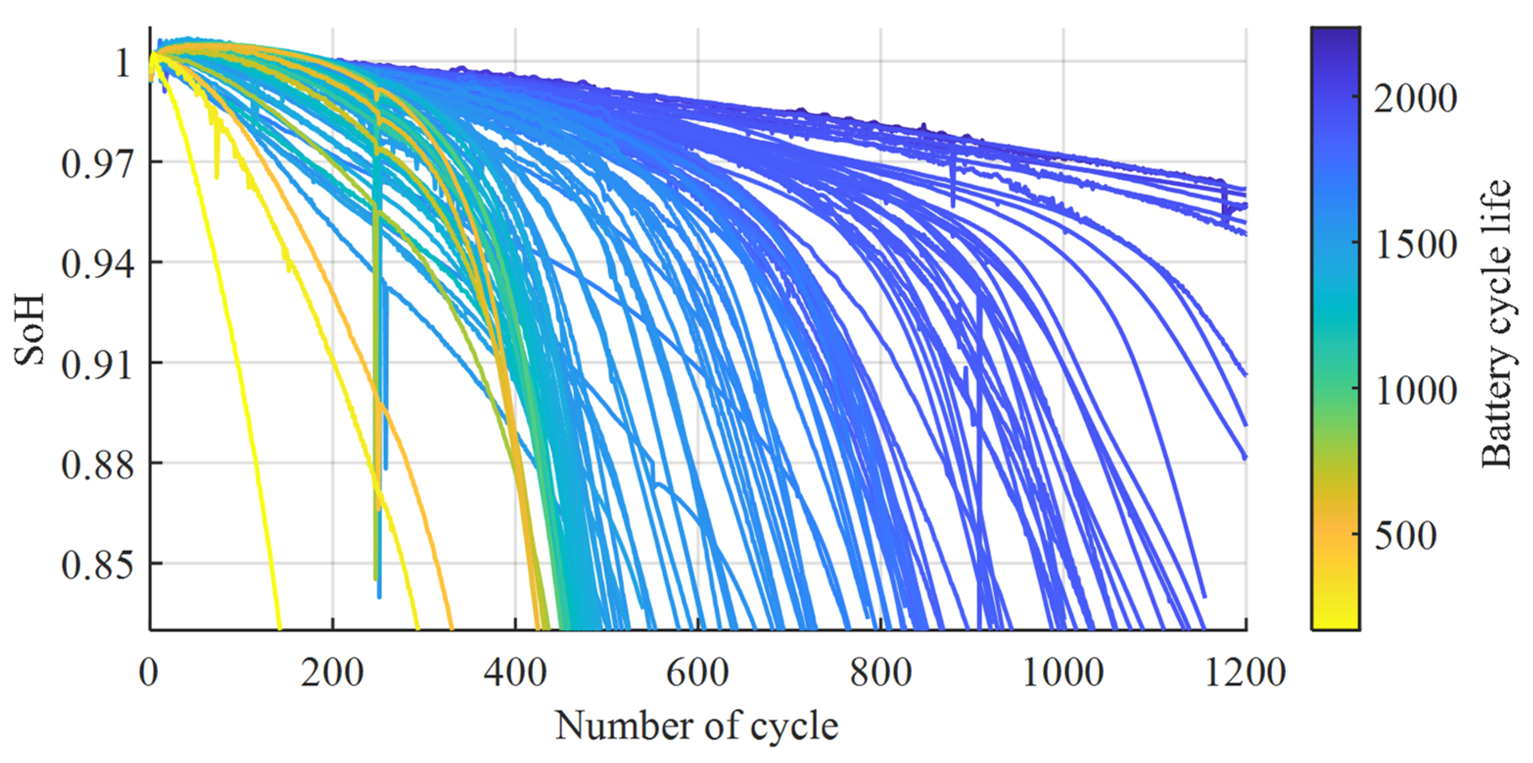
The number of cycles to failure for the batteries spans from approximately 150 to 2300, and the average end of life number is 806. Figure 1 shows the batteries ranked by cycle life, while Figure 2 shows the various SoH evolution profiles. The heterogeneous charging profiles generate a lot of variety within the dataset, allowing for deep analysis and insight into the behavior of the batteries and degradation patterns. For every battery cycle, the dataset includes a range of measured quantities including voltage, charge and discharge capacity, temperature, and internal resistance. In [14], the dataset authors created an in-depth analysis of the data and proposed many data-driven features, using which they developed a linear regression model to predict battery RUL.

3. Proposed Approach

This paper proposes a solution to estimate the SoH, which is based on a feature extraction procedure, where features that are considered strong battery health indicators are extracted from the discharge phase of every cycle. In the second step, those features are used as predictors to fit an SVR model, which is well suited to battery degradation modeling since it is strongly resistant to overfitting and can handle non-linear data. The SVR model is tuned with a cross-validation procedure and then used to perform SoH estimation.

3.1. Support Vector Regression

Support vector machine (SVM) is a very powerful algorithm for classification and regression tasks, which has been widely and successfully used in various fields such as image recognition, text classification, and prognostic and diagnostic processes. SVM works by finding the hyperplane that separates the data into classes and maximizes the minimum distance between data points and the hyperplane itself (maximizes the margin). SVM is effective with highly non-linear data thanks to the kernel trick: it can be used to transform the input (non-linear) data into higher-dimensional feature spaces, where linear classification can be performed.
SVR is a version of SVM specifically tailored for regression tasks. Similarly to SVM, it works by finding the hyperplane (line) that best fits the data and minimizes the error by using a tunable value ε as the minimum considered error. Any point lying inside the ε-tube is not considered in the cost function (1). A high value of ε leads to a more tolerant model, prone to underfitting, while a low value of ε leads to a more accurate but likely overfitted model. ξn, ξn* are the slack variables used to account for the positive and negative error of the points outside the ε-tube (2). The sum of ξn and ξn* is minimized in the loss function, weighted by a hyperparameter C, called a box constraint, which helps balance the complexity of the model. Finally, w and w′ are the weights arrays, normal and transposed, respectively; Yn is the target value; Xn′ is the transposed descriptor array; and b is the bias.
min 1 2   w w + C n = 1 N ( ξ n + ξ n * )
Y n X n w + b ε + ξ n     n X n w + b Y n   ε + ξ n   *   n

3.2. Feature Selection Procedure

In [10], the authors propose and study a set of features computed over the Toyota-MIT dataset, which they use as predictors to fit a linear regression model and provide an early RUL prediction at cycle 100 of the batteries. To do so, they extract one value of each feature per battery, using the measurements made between cycles 10 and 100. The extraction approach is revisited in this work and adapted to compute three of the features at every cycle. The values of the features are then used to feed the SVR model to obtain a continuous estimation of the SoH at every cycle, using the feature data of that cycle. The first two features are related to the discharge capacity curves of the batteries as a function of voltage (Q (V)), i.e., their total moved charge (Q) during each discharge phase.
Figure 3 shows these discharge capacity curves at different cycles of battery life. The area under each curve can be seen as the total energy output by the battery during that cycle, and it gradually drops as the battery ages. The discharge capacity curve at cycle 10 is taken as a reference to compute the values of the features. The reference discharge curve is then subtracted by the discharge curve of every cycle after it to obtain a measure of the drop in performance between cycle 10 and the actual cycle (k).
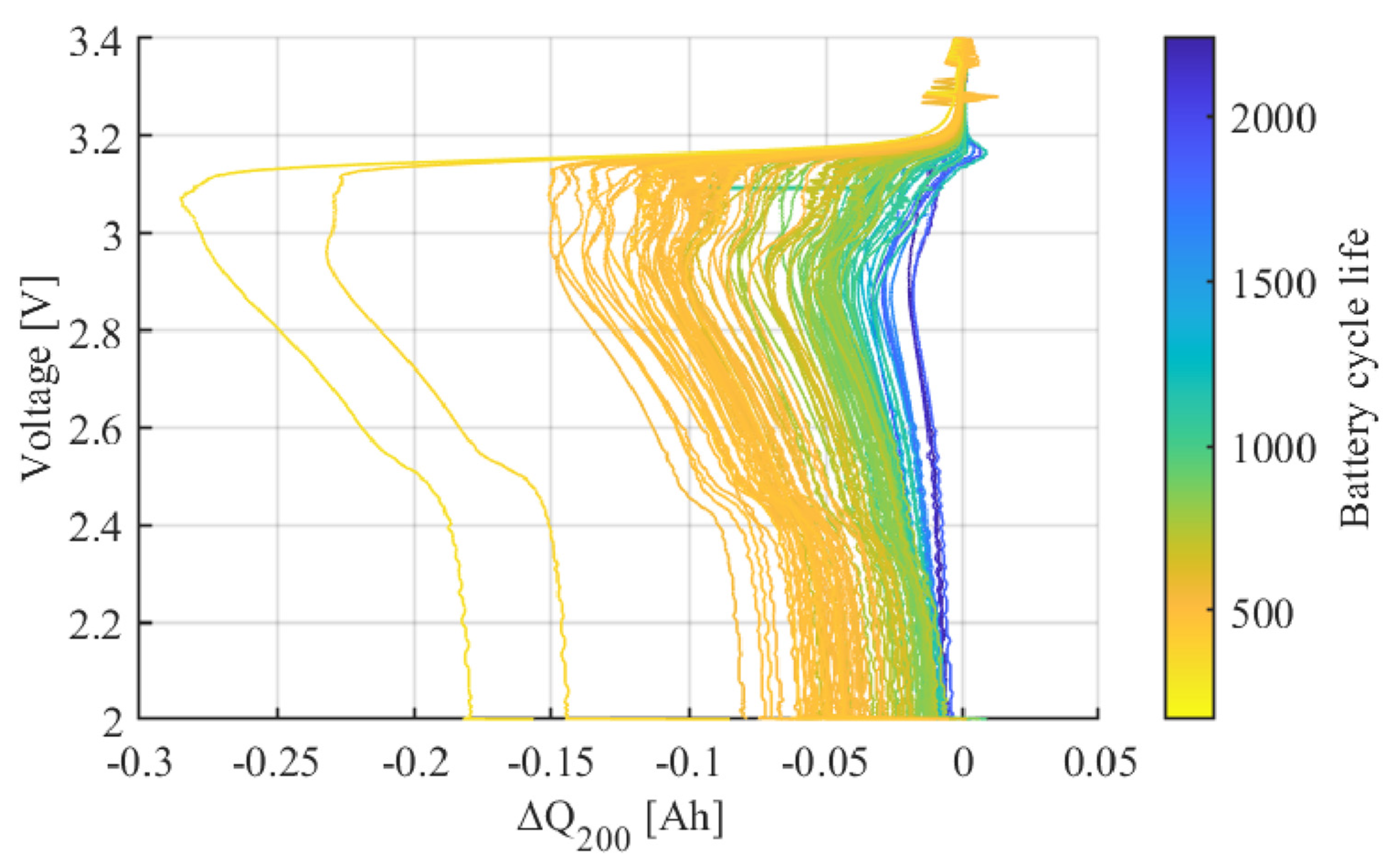
The full voltage range is equal for all the cycles (and batteries) and constitutes a solid base for comparisons. However, before it could be utilized, interpolation of the different curves over a common set of voltage values had to be performed so that their subtraction could be made point by point. In Figure 4, the difference curves are shown for cycle 200 of all batteries, which are the result of the procedure explained above. Blue lines that are almost flat show no significant drop in performance from cycle 10. Yellow lines, on the other hand, indicate a major degradation. The first feature (Ftr1) is computed as the common logarithm of the variance of the difference curves, while the second feature (Ftr2) is computed as the common logarithm of the minimum of the difference curves. Both the features are computed for every battery and every cycle except cycles from 1 to 10, for which the value is considered equal to the 11th. The result, for both features, is a feature space on which the data are almost linearly distributed over the battery life span, and it is plotted for cycle 200 of every battery in Figure 5a for Ftr1 and Figure 5b for Ftr2. This property is maintained over all the aging cycles. While the results for both features seem identical, drastic differences will come to the surface when partial discharge curves are discussed in Section 4.2.
Finally, the third feature (Ftr3) is computed as the sum of temperature: for every cycle k of each battery, the average temperature of each cycle ( T ¯ c y c l e ) is summed from the first up to the k-th cycle.
In Equation (3), the three features are defined and computed for each cycle of every battery. More specifically, Q10 (V) and Qk (V) represent the discharge capacities at reference cycle 10 and cycle k, respectively, as a function of voltage. ΔQk (V) is the difference of those two curves, while Δ Q k ¯ (V) represents the average value of that difference for cycle k. Parameter p refers to the number of points in the curve. Finally, Ti represents a singular temperature measurement.
F t r 1 ( k ) = l o g ( | 1 p 1 i = 1 p Δ Q k   V Δ Q k   ¯ V 2 | ) F t r 2 ( k ) = l o g ( | m i n ( Δ Q k   ( V   ) ) | ) F t r 3 ( k ) = c y c l e = 1 k T ¯ c y c l e Δ Q k   V = Q k   V Q 10   V Δ Q k ¯   V = 1 p i = 1 p Δ Q k , i V

4. Results and Discussion

4.1. Experimental Procedure and Full Discharge Window Approach

The voltage operating range of the batteries in the used dataset is approximately from 2 to 3.4 V. Initially, the features were extracted from the whole interval according to the procedure defined in Section 3.2. From the 124 available batteries, 15 were randomly selected to form the test set, while all of the cycles of the remaining 109 batteries formed the training and validation set. The SVR models were trained using solely the data of the 109 batteries. Initial parameter tuning was performed, followed by two sets of five-fold cross-validation (CV) campaigns to determine the best feature sets and then optimize the hyperparameters of the final model. In all stages, the predicted and measured values of SoH were compared after every cycle of every battery of the training and validation set.
To achieve a fully standardized and comparable results framework, the following procedure was developed and strictly followed:
The accuracy of the various proposed models was evaluated using the coefficient of determination (R2). It is often defined as the amount of variability in the data explained or accounted for by the model, and it is represented by Equation (4).
R 2 = 1 i = 1 n ( y i f ( x i ) ) 2 i = 1 n ( y i y ¯ ) 2
where
  • n—number of observations;
  • yi—target value of SoH;
  • f(xi)—predicted value of SoH;
  • y ¯ —mean of the target values.
Initial tuning of the SVR model hyperparameters (box constraint, epsilon, and kernel scale) was performed using MATLAB 2021b’s built-in tool for hyperparameter optimization with the following properties: Bayesian optimizer, 60 optimization iterations, and loss metric RMSE. Due to the limited computational power, the number of optimization iterations had to be limited as well. This step is required to find an acceptable starting point from which to proceed with subsequent refinements.
Afterward, one of three sets of features is selected, where each feature set is a different combination of the three constructed features. Five-fold cross-validation (CV) is applied to the three potential feature sets, and the one with the highest mean CV R2 is chosen. The considered feature sets along with their mean CV R2 scores for the full discharge window approach are shown in Table 1. The highest R2 value was achieved for feature set B, consisting of the first and third features.
Once the set of features is fixed, the model is further tuned by performing a five-fold CV for a range of values for each single hyperparameter, where the range depends on the results of the initial tuning of the parameters. This procedure is hierarchical, meaning that it starts from the most impactful hyperparameter (epsilon), then moves to the second most impactful (box constraint), and so on. The CV R2 of the final optimized model is 0.976. The hyperparameters of the final model considering the full window approach are a box constraint (BC) equal to 0.0055, epsilon equal to 0.0021, and a gaussian kernel and kernel scale (KS) of 1.
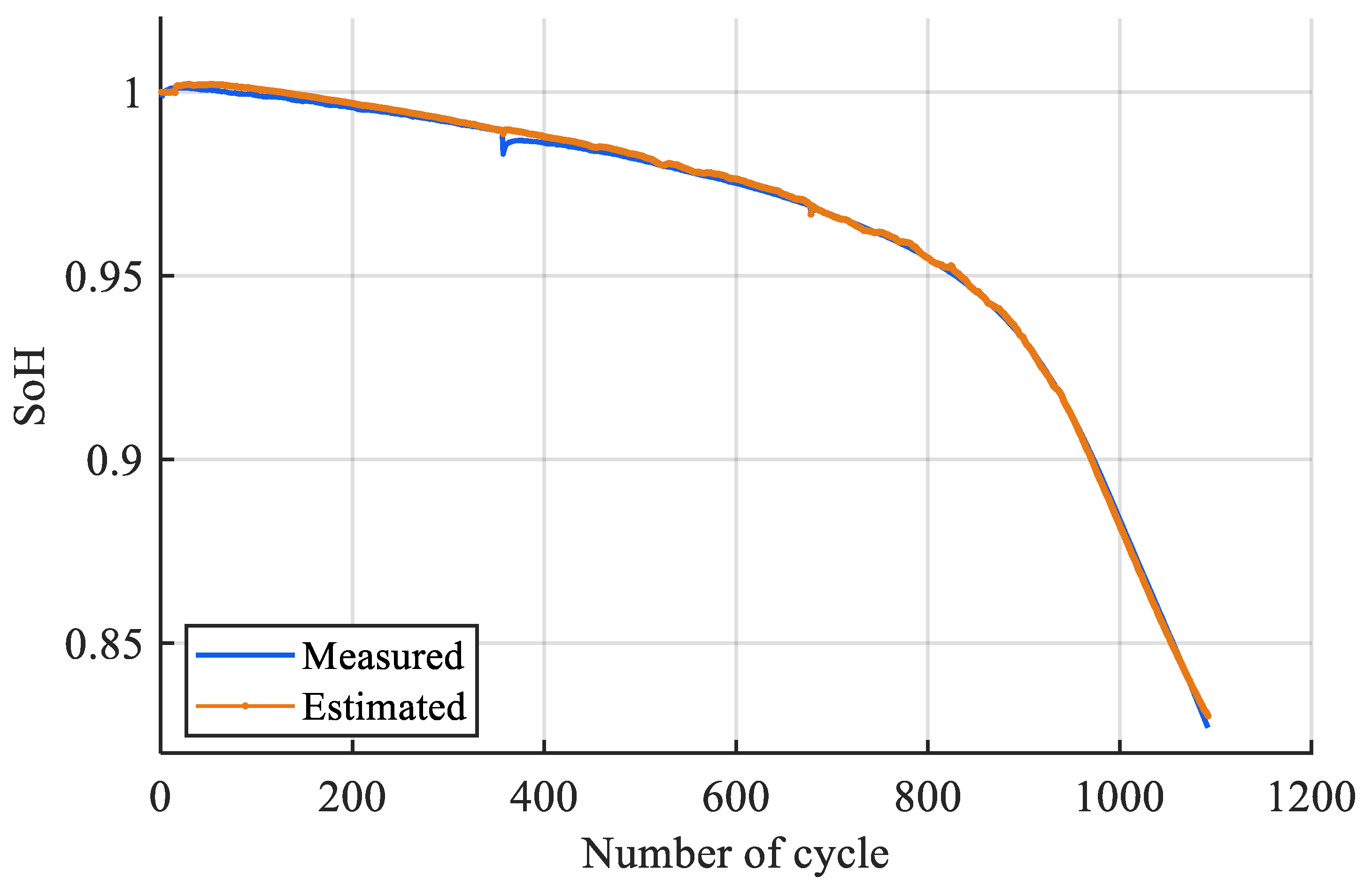
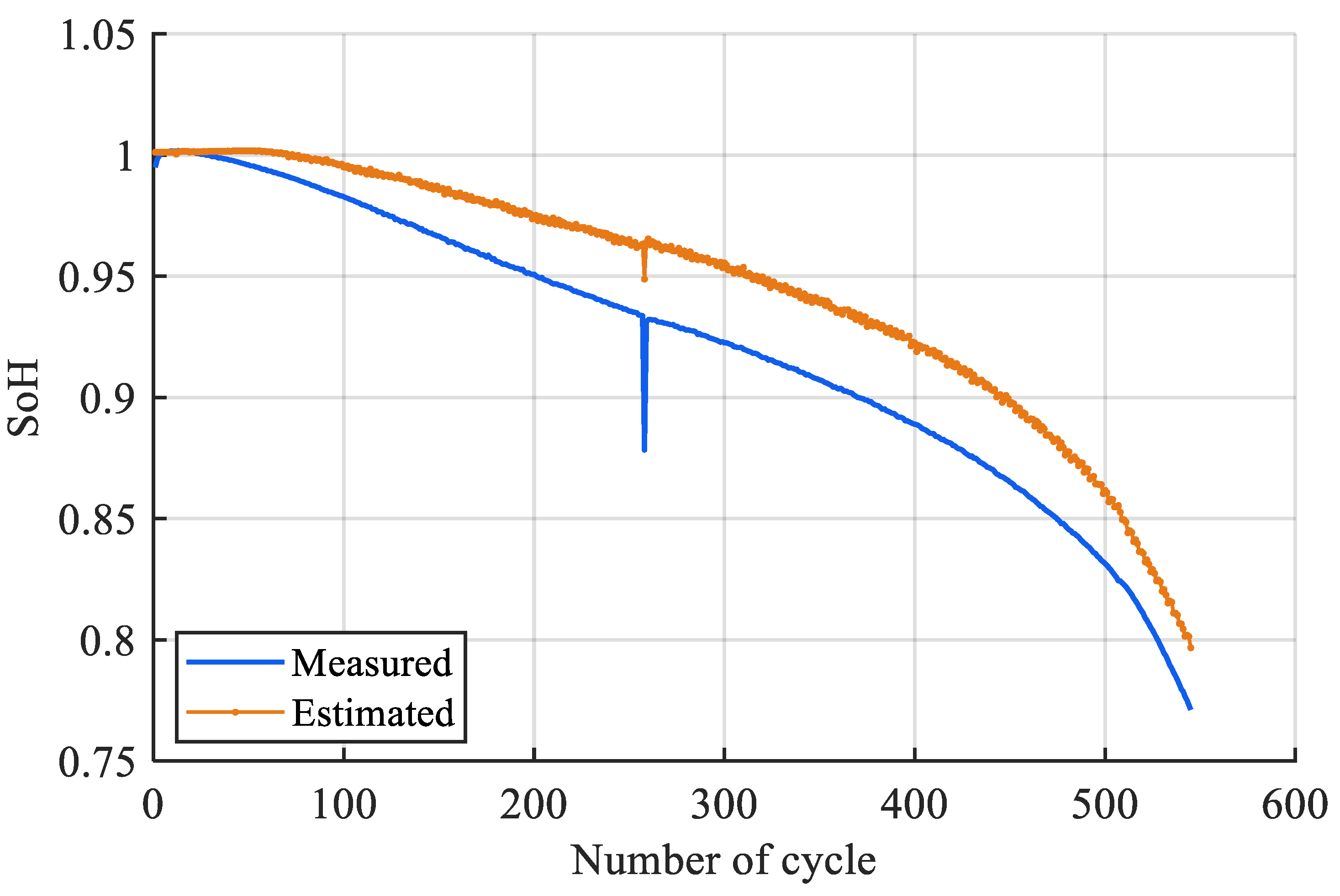
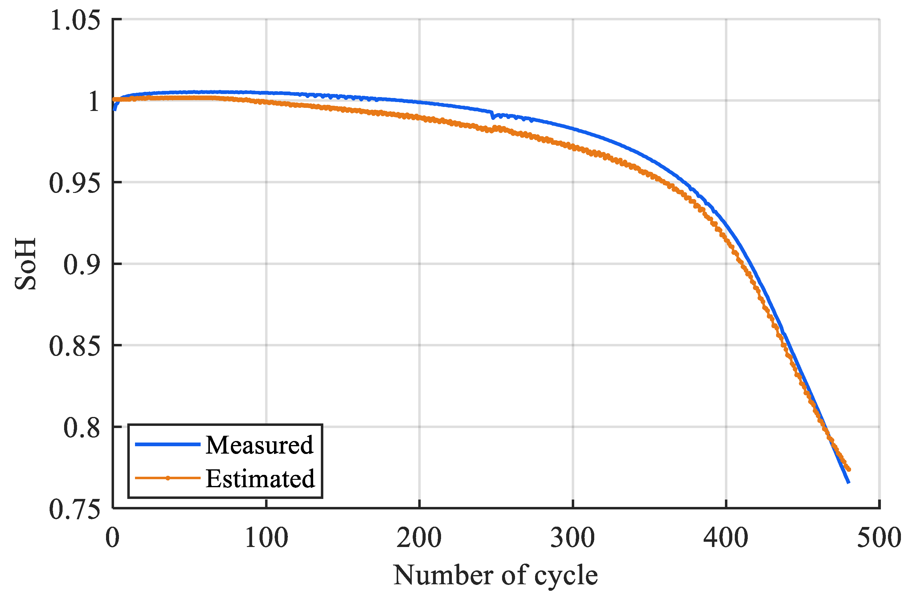
Finally, the test set is fed to the tuned model. In every cycle, the model provides a predicted value of the SoH based on the input data of the same cycle. The R2 value is calculated for every test battery individually, considering the measured and predicted value of the SoH after each cycle. The best fit is achieved for battery 11 (T11) of the test set, shown in Figure 6 with R2 = 0.999; the worst fit for battery 4 (T4), shown in Figure 7 with R2 = 0.794; and the mode is battery 5 (T5), shown in Figure 8 with an R2 = 0.981. The average R2 value for all batteries of the test set is also very high and equal to 0.962, indicating that, for the most part, the model fits the SoH evolution of the test set very well.

4.2. Partial Discharge Window Approach

The full window approach is subject to limitations in real use cases. The typical use of battery-powered devices prevents the battery cycle from adequately covering the entire voltage range since batteries are rarely fully charged and discharged. Therefore, further analysis was carried out, adopting the same experimental procedure described in Section 4.1. to study how performance is affected by shrinking and moving the adopted voltage window over the full voltage span.
Ten voltage intervals were selected and a five-fold CV procedure was performed for every voltage interval to choose the best feature set. The results in Table 2 demonstrate how the efficacy of the three feature sets changes for the different voltage intervals based on their R2 values. Moreover, the full voltage interval is also present in the table for comparison. For the high voltage intervals of 3.15 to 3.4 V and especially 3.25 to 3.4 V, which are highlighted in red, the R2 value is low for all feature sets. The explanation for this low accuracy can be found in Figure 3, which shows that between such high voltage limits the moved charge is low and does not profoundly change as the number of cycles increase, thereby resulting in suboptimal features. Table 2 also shows that feature set B performs poorly for voltage intervals with an upper limit of less than 3.1 V. One of the features of this set is related to the variance in the difference between the curves of cycle k and the reference cycle 10. While this set was the best performer in the case of a full voltage window, it can be seen in Figure 4 that these difference curves have a constant value for voltages lower than 3.1 and, thus, the variance is no longer a good indicator. On the other hand, this is not the case for the minimum of the difference curve; thus, feature sets C and A continue to perform well. For each voltage interval, the feature set that results in the highest R2 value is selected. The chosen feature set along with the final tuned value of the hyperparameter for each model are shown in Table 3.
Table 4 shows a five-fold CV procedure applied on the final models. The results show very repeatable R2 values for all folds and all voltage intervals except for 3.15–3.4 V and 3.25–3.4 V. For all other intervals, the minimum R2 value of any fold is higher than 0.91, and the mean R2 value across all folds ranges between 0.957 and 0.982. These results demonstrate that for the training and validation data, the models are of appropriate complexity and have low bias and variance. This is further corroborated when the models are applied to the remaining test battery data, as shown in Table 5.
The columns of Table 5 are the different voltage intervals used to build the features of the final models, while the rows are each test battery. As was the case for the full voltage window, the R2 value shows the accuracy with which the predicted value of SoH—as a function of the number of cycles—compares with the measured one, for every battery individually. Unsurprisingly, for the voltage ranges of 3.15–3.4 V and 3.25–3.4 V, the accuracy of the models is low for most batteries. On the other hand, for the rest of the intervals, the R2 values are high and similar to the full window, and to the R2 values obtained during the five-fold CV campaign using the training and validation data. More specifically, the mean R2 for all batteries is in the range of 0.939 and 0.973. Therefore, the first conclusion is that the models are accurate and not just overfitting to the training data. The second, but just as important, conclusion is that partial voltage ranges can be used to build the features of the model, thus giving real-life applicability to the constructed models.
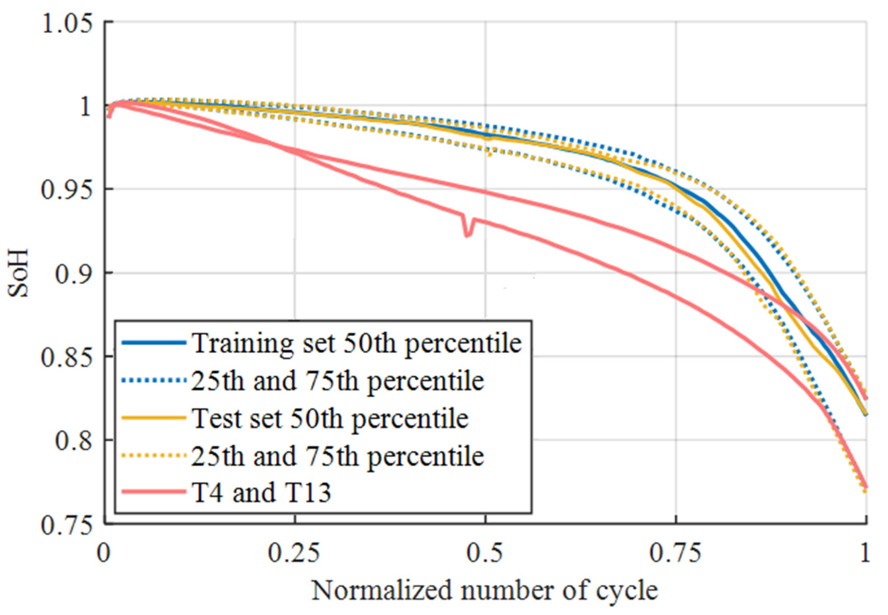
Finally, it can be noted that for batteries 13 (T13) and 4 (T4), highlighted in red in Table 5, the model accuracy is not very high, regardless of the voltage range used. This is because they follow a very different SoH evolution trend. To highlight this difference, for every battery, the SoH as a function-normalized number of cycles was defined by dividing the value of number of cycles by the value of total number of cycles. Therefore, the normalized number of cycles value for all cells is equal to 0 at the beginning and 1 when the battery reaches the end of life. Afterwards, the batteries of the training and validation set are grouped by their SoH value at every percent of the normalized number of cycles. The blue curve in Figure 9 is the 50th percentile for the SoH as a function of the normalized number of cycles, while the dotted blue lines are the 25th and 75th percentile. The same procedure is repeated for the test set, omitting T4 and T13. The yellow line is the 50th percentile of the SoH evolution for the test set, while the yellow dotted lines are the 25th and 75th percentile. Based on the small width of the percentile curves, as well as the mostly overlapping blue and yellow curves, it can be concluded that the batteries of the train and test set follow a similar SoH evolution trend, regardless of their vastly different cycle life. On the contrary, batteries 4 and 13, represented by the two red curves in Figure 9, follow a vastly different pattern of degradation, having a more sudden and almost linear decline in SoH rather than a slow descent. This is most likely due to some physical internal battery issue or extreme usage conditions, making these two cells outliers of the dataset and resulting in lower accuracy of SoH estimation by the models.

5. Conclusions

Accurate battery SoH estimation is crucial to achieve optimal performance, ensure safety, and minimize cost and environmental impact. This paper presents an SoH estimation method based on SVR, which offers a favorable compromise between applicability, computational efficiency, and accuracy of results. The dataset used in this work consists of 124 batteries. A total 109 batteries formed the training and validation set and the remaining 15 batteries formed the test set, which was used only in the final stage, to evaluate the performance of the developed models. Three features were selected, including two derived from discharge capacity curves and the third one based on battery temperature.
Moreover, three combinations of features were analyzed to determine how their effectiveness changes across different voltage ranges. When full discharge capacity curves are considered, all three feature combinations are successful, with the best results obtained when considering the logarithm of the variance of the difference curves and the temperature integral features, reaching a mean CV R2 value of 0.976 for the training set and 0.962 for the test set. Additionally, the same features were built from 10 small voltage intervals, and the results show the considerations that must be made when following this approach—namely, models using features constructed from the upper voltage limits of 3.15–3.4 V or 3.25–3.4 V demonstrate poor accuracy because at such high voltage limits the moved charge is low and does not profoundly change as the number of cycles increases. Furthermore, feature set B performs poorly for voltage intervals with an upper limit of less than 3.1 V because the difference curves have a constant value for voltages lower than 3.1 V; thus, the feature related to variance is no longer a good indicator. This is not the case for the minimum of the difference curve feature; thus, feature sets A and C continue to perform well. The models that incorporate these limitations are very successful, reaching a CV R2 value in the range of 0.957 and 0.982, and a mean R2 value for the test set in the range of 0.939 and 0.973, depending on the selected voltage interval. These values are on par with the values achieved considering the full voltage window. Therefore, it can be concluded that partial voltage ranges can be used to build the features of the model, thus giving real-life applicability to the constructed models.

Author Contributions

Conceptualization, E.P., I.M. and L.C.; methodology, E.P. and I.M.; software, I.M. and E.P.; validation, I.M. and M.F.; formal analysis, E.P.; investigation, I.M.; resources, E.P.; data curation, L.C. and E.P.; writing—original draft preparation, E.P. and I.M; writing—review and editing, E.P. and I.M.; visualization, E.P. and I.M.; supervision, L.C., M.F. and E.P.; project administration, L.C. and M.F.; funding acquisition, L.C. and M.F. All authors have read and agreed to the published version of the manuscript.

Funding

The research received no external funding.

Data Availability Statement

Data are contained within the article.

Conflicts of Interest

The authors declare no conflicts of interest.

References

  1. Pelletier, S.; Jabali, O.; Laporte, G.; Veneroni, M. Battery Degradation and Behaviour for Electric Vehicles: Review and Numerical Analyses of Several Models. Transp. Res. Part B Methodol. 2017, 103, 158–187. [Google Scholar] [CrossRef]
  2. Cristaldi, L.; Faifer, M.; Laurano, C.; Ottoboni, R.; Petkovski, E.; Toscani, S. Power Generation Control Algorithm for the Participation of Photovoltaic Panels in Network Stability. IEEE Trans. Instrum. Meas. 2023, 72, 9000809. [Google Scholar] [CrossRef]
  3. Li, X.; Fan, G.; Rizzoni, G.; Canova, M.; Zhu, C.; Wei, G. A Simplified Multi-Particle Model for Lithium Ion Batteries Via a Predictor-Corrector Strategy and Quasi-Linearization. Energy 2016, 116, 154–169. [Google Scholar] [CrossRef]
  4. Petit, M.; Prada, E.; Sauvant-Moynot, V. Development of an Empirical Aging Model for Li-Ion Batteries and Application to Assess the Impact of Vehicle-to-Grid Strategies on Battery Lifetime. Appl. Energy 2016, 172, 398–407. [Google Scholar] [CrossRef]
  5. Barcellona, S.; Colnago, S.; Dotelli, G.; Latorrata, S.; Piegari, L. Aging Effect on the Variation of Li-Ion Battery Resistance as Function of Temperature and State of Charge. J. Energy Storage 2022, 50, 104658. [Google Scholar] [CrossRef]
  6. Xu, B.; Oudalov, A.; Ulbig, A.; Andersson, G.; Kirschen, D.S. Modeling of Lithium-Ion Battery Degradation for Cell Life Assessment. IEEE Trans. Smart Grid 2018, 9, 1131–1140. [Google Scholar] [CrossRef]
  7. Li, X.; Yuan, C.; Li, X.; Wang, Z. State of Health Estimation for Li-Ion Battery Using Incremental Capacity Analysis and Gaussian Process Regression. Energy 2020, 190, 116467. [Google Scholar] [CrossRef]
  8. Cui, Z.; Wang, C.; Gao, X.; Tian, S. State of Health Estimation for Lithium-Ion Battery Based on the Coupling-Loop Nonlinear Autoregressive with Exogenous Inputs Neural Network. Electrochim. Acta 2021, 393, 139047. [Google Scholar] [CrossRef]
  9. Cao, M.; Zhang, T.; Wang, J.; Liu, Y. A Deep Belief Network Approach to Remaining Capacity Estimation for Lithium-Ion Batteries Based on Charging Process Features. J. Energy Storage 2022, 48, 103825. [Google Scholar] [CrossRef]
  10. Severson, K.A.; Attia, P.M.; Jin, N.; Perkins, N.; Jiang, B.; Yang, Z.; Chen, M.H.; Aykol, M.; Herring, P.K.; Fraggedakis, D.; et al. Data-Driven Prediction of Battery Cycle Life before Capacity Degradation. Nat. Energy 2019, 4, 383–391. [Google Scholar] [CrossRef]
  11. Ansean, D.; Garcia, V.M.; Gonzalez, M.; Blanco-Viejo, C.; Viera, J.C.; Pulido, Y.F.; Sanchez, L. Lithium-Ion Battery Degradation Indicators Via Incremental Capacity Analysis. IEEE Trans. Ind. Appl. 2019, 55, 2992–3002. [Google Scholar] [CrossRef]
  12. He, J.; Wei, Z.; Bian, X.; Yan, F. State-of-Health Estimation of Lithium-Ion Batteries Using Incremental Capacity Analysis Based on Voltage–Capacity Model. IEEE Trans. Transp. Electrif. 2020, 6, 417–426. [Google Scholar] [CrossRef]
  13. Zhou, R.; Zhu, R.; Huang, C.-G.; Peng, W. State of Health Estimation for Fast-Charging Lithium-Ion Battery Based on Incremental Capacity Analysis. J. Energy Storage 2022, 51, 104560. [Google Scholar] [CrossRef]
  14. Richardson, R.R.; Birkl, C.R.; Osborne, M.A.; Howey, D.A. Gaussian Process Regression for In Situ Capacity Estimation of Lithium-Ion Batteries. IEEE Trans. Ind. Inform. 2019, 15, 127–138. [Google Scholar] [CrossRef]
  15. Richardson, R.R.; Osborne, M.A.; Howey, D.A. Gaussian Process Regression for Forecasting Battery State of Health. J. Power Sources 2017, 357, 209–219. [Google Scholar] [CrossRef]
  16. Jia, J.; Liang, J.; Shi, Y.; Wen, J.; Pang, X.; Zeng, J. SOH and RUL Prediction of Lithium-Ion Batteries Based on Gaussian Process Regression with Indirect Health Indicators. Energies 2020, 13, 375. [Google Scholar] [CrossRef]
  17. Barcellona, S.; Cristaldi, L.; Faifer, M.; Petkovski, E.; Piegari, L.; Toscani, S. State of Health Prediction of Lithium-Ion Batteries. In Proceedings of the 2021 IEEE International Workshop on Metrology for Industry 4.0 & IoT (MetroInd4.0 & IoT), Rome, Italy, 7–9 June 2021; pp. 12–17. [Google Scholar]
  18. Lashgari, F.; Petkovski, E.; Cristaldi, L. State of Health Analysis for Lithium-Ion Batteries Considering Temperature Effect. In Proceedings of the 2022 IEEE International Workshop on Metrology for Extended Reality, Artificial Intelligence and Neural Engineering (MetroXRAINE 2022-Proceedings), Rome, Italy, 26–28 October; pp. 40–45. [CrossRef]
  19. Weng, C.; Sun, J.; Peng, H. Model Parametrization and Adaptation Based on the Invariance of Support Vectors With Applications to Battery State-of-Health Monitoring. IEEE Trans. Veh. Technol. 2015, 64, 3908–3917. [Google Scholar] [CrossRef]
  20. Feng, X.; Weng, C.; He, X.; Han, X.; Lu, L.; Ren, D.; Ouyang, M. Online State-of-Health Estimation for Li-Ion Battery Using Partial Charging Segment Based on Support Vector Machine. IEEE Trans. Veh. Technol. 2019, 68, 8583–8592. [Google Scholar] [CrossRef]
  21. Marri, I.; Petkovski, E.; Cristaldi, L.; Faifer, M. Lithium-Ion Batteries Soh Estimation, Based on Support-Vector Regression and a Feature-Based Approach. In Proceedings of the 18th IMEKO TC10 Conference on Measurement for Diagnostic, Optimisation and Control to Support Sustainability and Resilience 2022, Warsaw, Poland, 26–27 September 2022; pp. 109–113. [Google Scholar]
  22. Marri, I.; Petkovski, E.; Cristaldi, L.; Faifer, M. Comparing Machine Learning Strategies for SoH Estimation of Lithium-Ion Batteries Using a Feature-Based Approach. Energies 2023, 16, 4423. [Google Scholar] [CrossRef]
  23. Wen, J.; Chen, X.; Li, X.; Li, Y. SOH Prediction of Lithium Battery Based on IC Curve Feature and BP Neural Network. Energy 2022, 261, 125234. [Google Scholar] [CrossRef]
  24. Tian, Y.; Dong, Q.; Tian, J.; Li, X.; Kukkapalli, V.K.; Kim, S.; Thomas, S.A. Capacity Estimation of Lithium-Ion Batteries Based on Multiple Small Voltage Sections and BP Neural Networks. Energies 2023, 16, 674. [Google Scholar] [CrossRef]
  25. Li, Y.; Li, K.; Liu, X.; Wang, Y.; Zhang, L. Lithium-Ion Battery Capacity Estimation—A Pruned Convolutional Neural Network Approach Assisted with Transfer Learning. Appl. Energy 2021, 285, 116410. [Google Scholar] [CrossRef]
  26. Catelani, M.; Ciani, L.; Fantacci, R.; Patrizi, G.; Picano, B. Remaining Useful Life Estimation for Prognostics of Lithium-Ion Batteries Based on Recurrent Neural Network. IEEE Trans. Instrum. Meas. 2021, 70, 3524611. [Google Scholar] [CrossRef]
  27. Marri, I.; Petkovski, E.; Cristaldi, L.; Faifer, M. Battery Remaining Useful Life Prediction Supported by Long Short-Term Memory Neural Network. In Proceedings of the IEEE International Instrumentation and Measurement Technology Conference (I2MTC), Kuala Lumpur, Malaysia, 22–25 May 2023; pp. 1–6. [Google Scholar] [CrossRef]
  28. Qu, J.; Liu, F.; Ma, Y.; Fan, J. A Neural-Network-Based Method for RUL Prediction and SOH Monitoring of Lithium-Ion Battery. IEEE Access 2019, 7, 87178–87191. [Google Scholar] [CrossRef]
  29. Tan, Y.; Zhao, G. Transfer Learning with Long Short-Term Memory Network for State-of-Health Prediction of Lithium-Ion Batteries. IEEE Trans. Ind. Electron. 2020, 67, 8723–8731. [Google Scholar] [CrossRef]
  30. Wang, S.; Takyi-Aninakwa, P.; Jin, S.; Yu, C.; Fernandez, C.; Stroe, D.-I. An Improved Feedforward-Long Short-Term Memory Modeling Method for the Whole-Life-Cycle State of Charge Prediction of Lithium-Ion Batteries Considering Current-Voltage-Temperature Variation. Energy 2022, 254, 124224. [Google Scholar] [CrossRef]
  31. Wang, S.; Wu, F.; Takyi-Aninakwa, P.; Fernandez, C.; Stroe, D.-I.; Huang, Q. Improved Singular Filtering-Gaussian Process Regression-Long Short-Term Memory Model for Whole-Life-Cycle Remaining Capacity Estimation of Lithium-Ion Batteries Adaptive to Fast Aging and Multi-Current Variations. Energy 2023, 284, 128677. [Google Scholar] [CrossRef]
  32. Toyota Research Institute. Experimental Data Platform. 2021. Available online: https://data.matr.io/1/ (accessed on 1 September 2023).
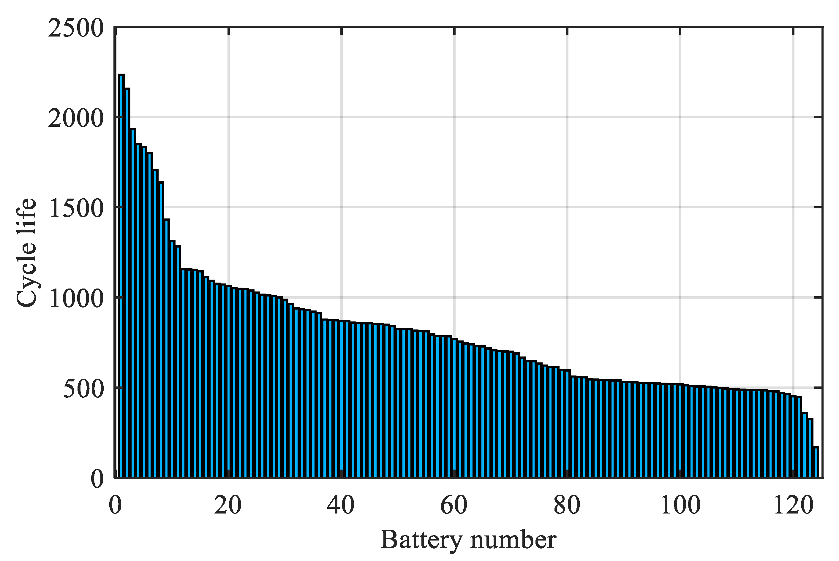
Figure 1. Dataset ordered by battery lifespan expressed in number of cycles.
Energies 17 00206 g001
Figure 2. SoH over number of cycles for a set of representative batteries of the dataset.
Energies 17 00206 g002
Figure 3. Discharging capacity as a function of voltage for all cycles of a sample battery.
Energies 17 00206 g003
Figure 4. Difference in discharge capacity curves between reference cycle 10 and cycle 200, calculated for all the batteries.
Energies 17 00206 g004
Figure 5. (a) Common logarithm of the variance in the difference between capacity curves at cycle 200 and cycle 10 for all batteries (Ftr1(200)). (b) Common logarithm of the minimum of the difference between capacity curves at cycle 200 and cycle 10 for all batteries (Ftr2(200)).
Energies 17 00206 g005
Figure 6. Best SoH estimation results for test battery 11.
Energies 17 00206 g006
Figure 7. Worst SoH estimation results for test battery 4.
Energies 17 00206 g007
Figure 8. Mode SoH estimation results for test battery 5.
Energies 17 00206 g008
Figure 9. Distribution of the SoH evolution curves for the training data (blue), test data (yellow), and mis-predicted batteries 4 and 13 (red).
Energies 17 00206 g009
Table 1. Feature sets and achieved R2 values.
Feature SetFeaturesMean CV R2
AFtr1, Ftr2, Ftr30.968
BFtr1, Ftr30.970
CFtr2, Ftr30.961
Table 2. Mean cross-validation R2 values for feature set selection.
Voltage Range (V)Feature Set AFeature Set B Feature Set C
Full window (2–3.4)0.96860.97050.9620
3–3.40.88520.95720.9538
3.15–3.40.89920.83060.8777
3.25–3.40.85170.78940.8195
3–3.20.96240.96450.9536
3–3.10.94290.39040.9531
3–3.050.96080.38830.9646
2.8–30.96910.47150.9705
2.9–30.96570.39320.9705
2.4–2.60.97740.39440.9699
2.2–2.40.97720.32690.9741
Table 3. Final model hyperparameters for every voltage interval.
Voltage Range (V)BCKSEpsilonKernelFeature Set
Full window (2–3.4)0.00551.00.0021GaussianB
3–3.40.00551.00.0005GaussianB
3.15–3.41.1002.00.0001GaussianA
3.25–3.40.0221.00.0021GaussianA
3–3.20.00551.00.0001GaussianB
3–3.10.00551.00.0010GaussianC
3–3.050.00551.00.0021GaussianC
2.8–30.00551.00.00005GaussianC
2.9–30.00551.00.0010GaussianC
2.4–2.60.11002.00.0010GaussianA
2.2–2.40.11002.00.0005GaussianA
Table 4. Five-fold CV R2 values of the final model for every voltage interval.
Voltage Range (V)Fold 1Fold 2Fold 3Fold 4Fold 5Mean
Full window (2–3.4)0.95780.96820.98910.98360.98160.9761
3–3.40.93370.95540.97990.96510.97010.9609
3.15–3.40.86720.91090.89940.91350.93010.9042
3.25–3.40.80630.82060.91460.87170.84950.8525
3–3.20.94790.95890.98460.97450.97070.9673
3–3.10.94530.91130.97840.97490.97350.9567
3–3.050.95090.96140.98160.97530.97420.9687
2.8–30.95850.96520.98570.98040.98020.9740
2.9–30.95810.96530.98550.98000.97970.9737
2.4–2.60.97840.97220.98420.98930.98660.9821
2.2–2.40.97600.97180.98930.98500.98650.9818
Table 5. R2 value of all 15 test batteries for all selected voltage intervals.
Full Window3–3.43.25–3.43.15–3.43–3.23–3.13–3.052.8–32.9–32.4–2.62.2–2.4
T10.98340.94340.6180.56220.95140.95480.96440.97440.97520.98740.9839
T20.98320.93710.98260.87650.95270.95120.95300.96650.96600.99130.9970
T30.99450.99010.99150.97340.99080.99140.99060.99140.99150.99540.9919
T40.79380.78170.77880.74520.75980.76890.78550.80380.80430.81030.8133
T50.98130.98690.98510.87840.98350.98870.98690.98530.98560.97820.9704
T60.97710.97730.96780.74700.88240.97370.97170.97090.97180.99050.9948
T70.94800.89370.76680.88380.90070.92160.93050.94650.94710.99240.9910
T80.99760.97710.66770.96130.99780.97830.97710.99660.99520.99870.9996
T90.99450.98250.95000.95210.99000.98960.98960.99240.99240.99700.9977
T100.99630.97960.86330.84680.97750.99250.99370.99670.99670.98810.9995
T110.99920.99850.82780.99640.99920.99900.99880.99930.99920.99810.9993
T120.97090.95330.89230.9610.93610.94270.94550.95540.95370.99620.9891
T130.82340.81260.53290.67320.79520.81330.81960.81330.80890.87350.8706
T140.99250.97630.99290.95030.97820.97960.98050.98860.98850.99840.9987
T150.99440.98090.89170.95050.98560.98350.98560.98720.98800.99580.9954
Mean0.96200.94470.84730.86390.93870.94860.95150.95790.95760.97270.9728
Disclaimer/Publisher’s Note: The statements, opinions and data contained in all publications are solely those of the individual author(s) and contributor(s) and not of MDPI and/or the editor(s). MDPI and/or the editor(s) disclaim responsibility for any injury to people or property resulting from any ideas, methods, instructions or products referred to in the content.