
Recursive Neural Network as a Multiple Input–Multiple Output Speed Controller for Electrical Drive of Three-Mass System


Abstract
:1. Introduction
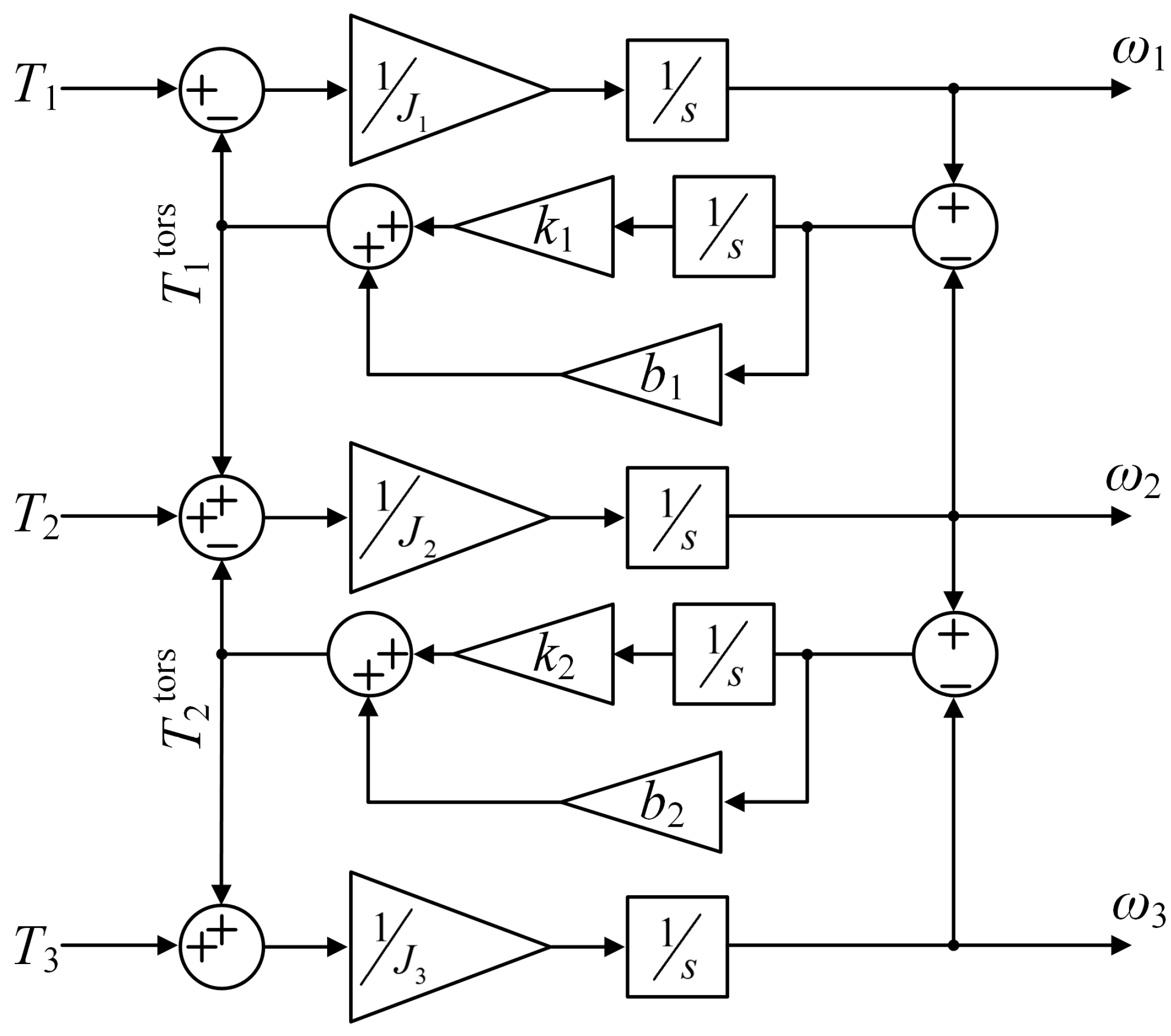
2. Mathematical Description of the Three-Mass System
3. Control System Structure
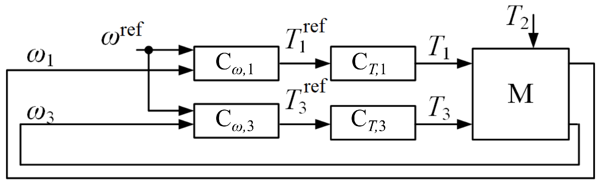
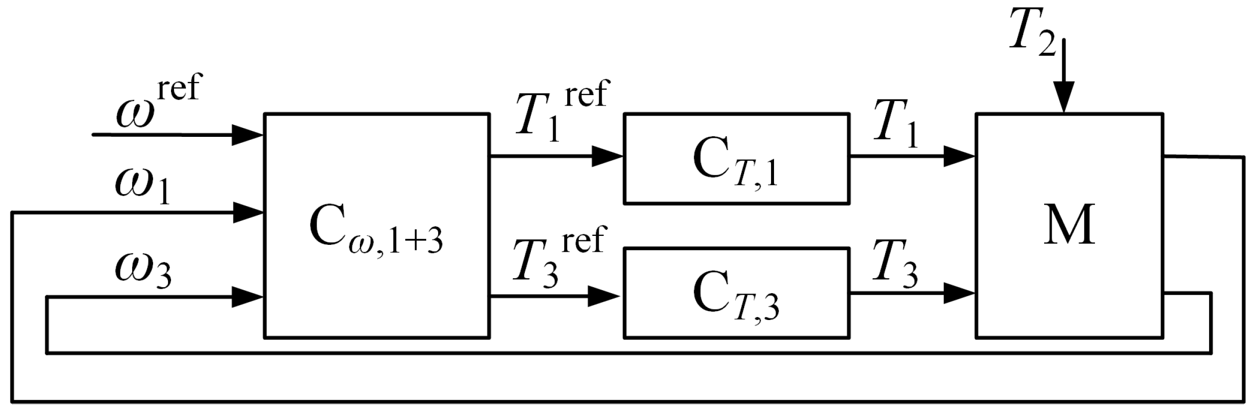
3.1. Reference Control Structure
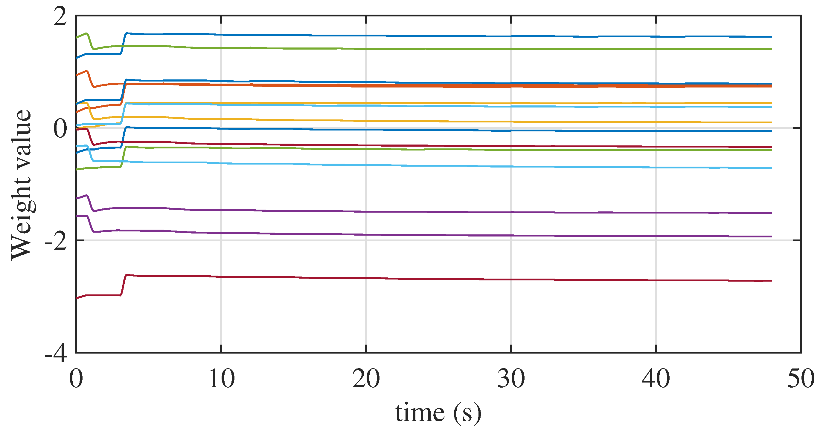
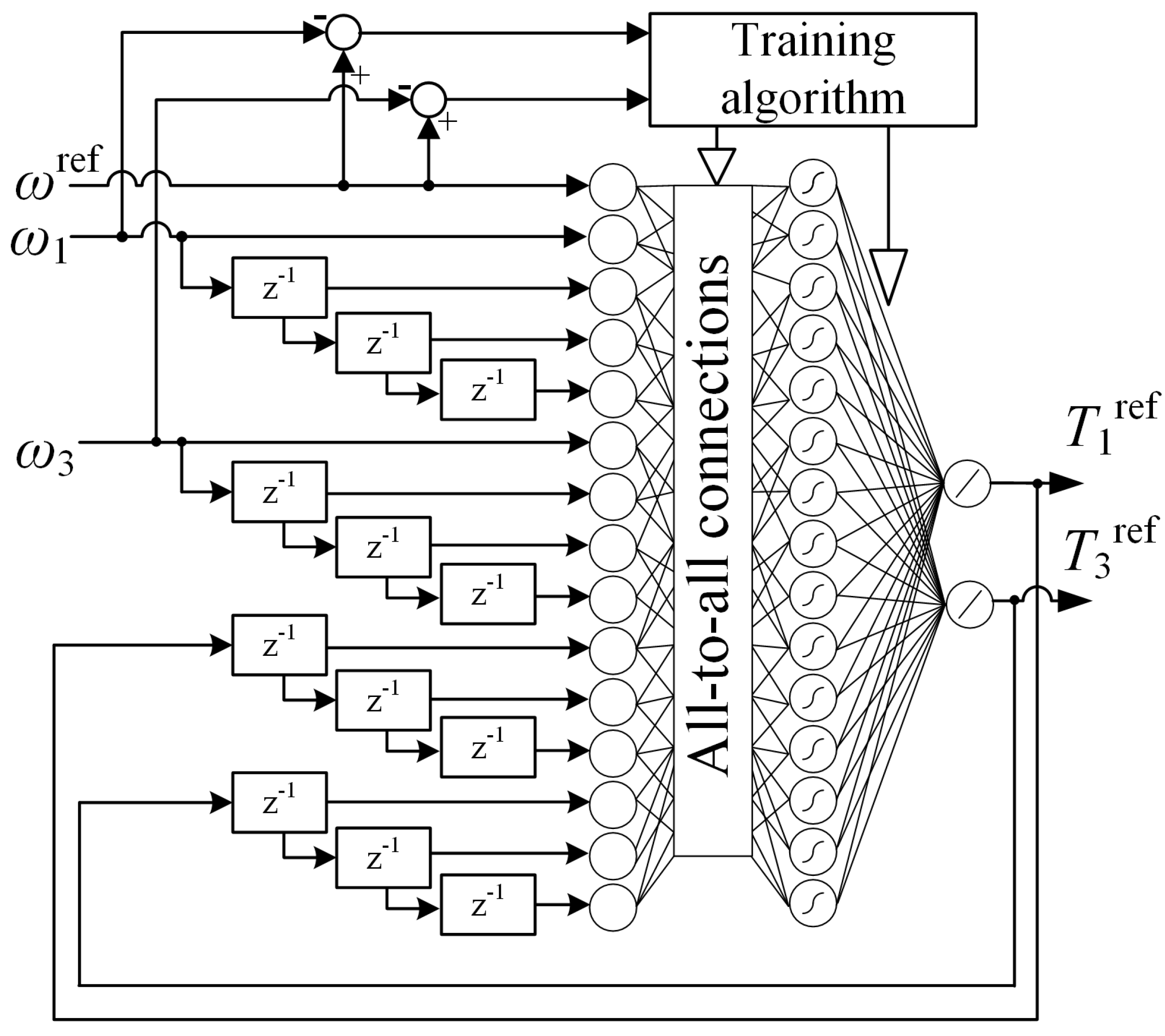
3.2. ANN Speed Controller
- Reference speed that is common for both motors ();
- feedback signal taken from the encoder of motor no. 1 and its previous samples (, ,…, );
- Feedback signal taken from the encoder of motor no. 2 and its previous samples (, ,…, );
- Past samples of the output signals (reference torques , ,…, and , ,…, ).
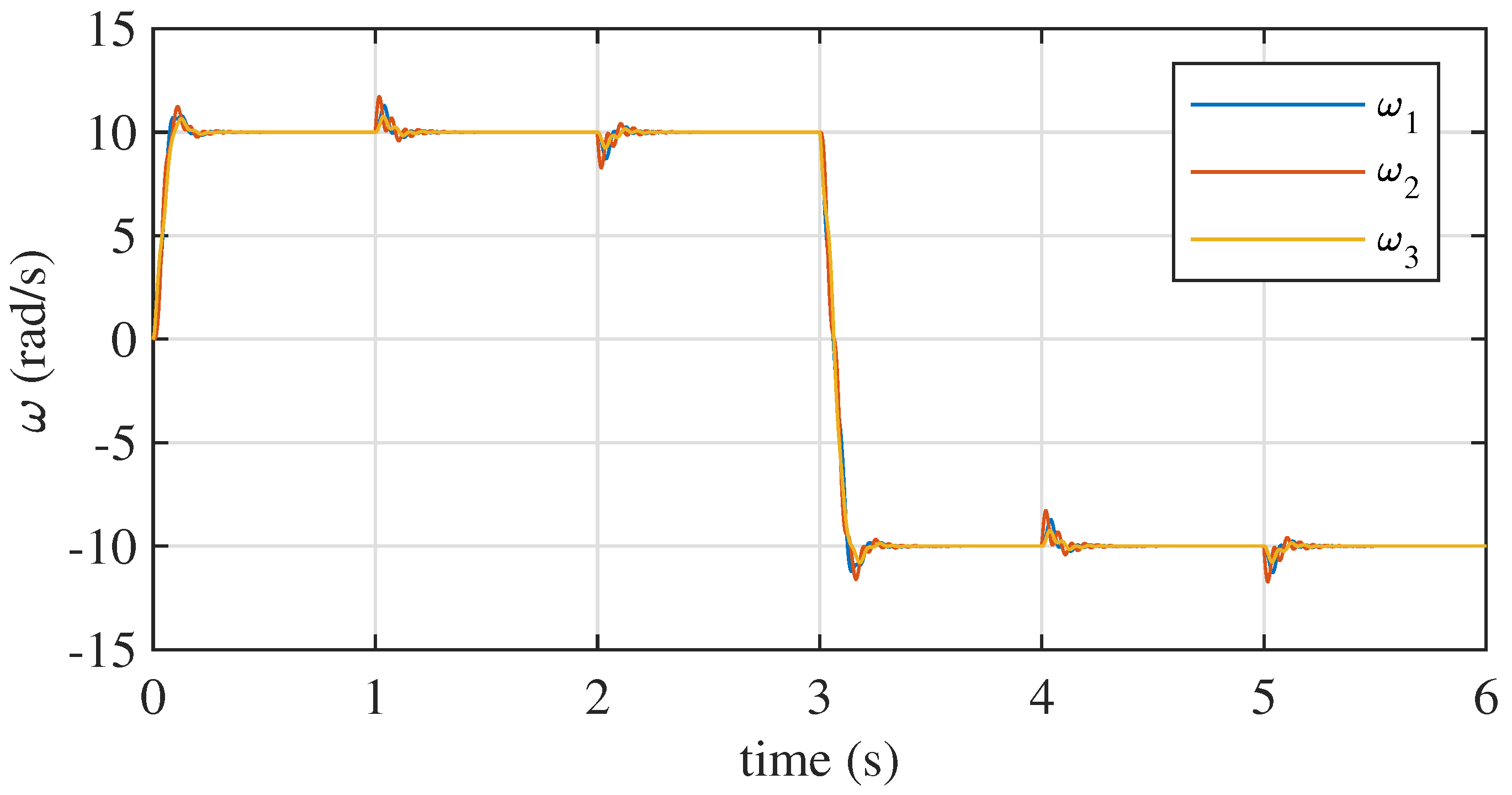
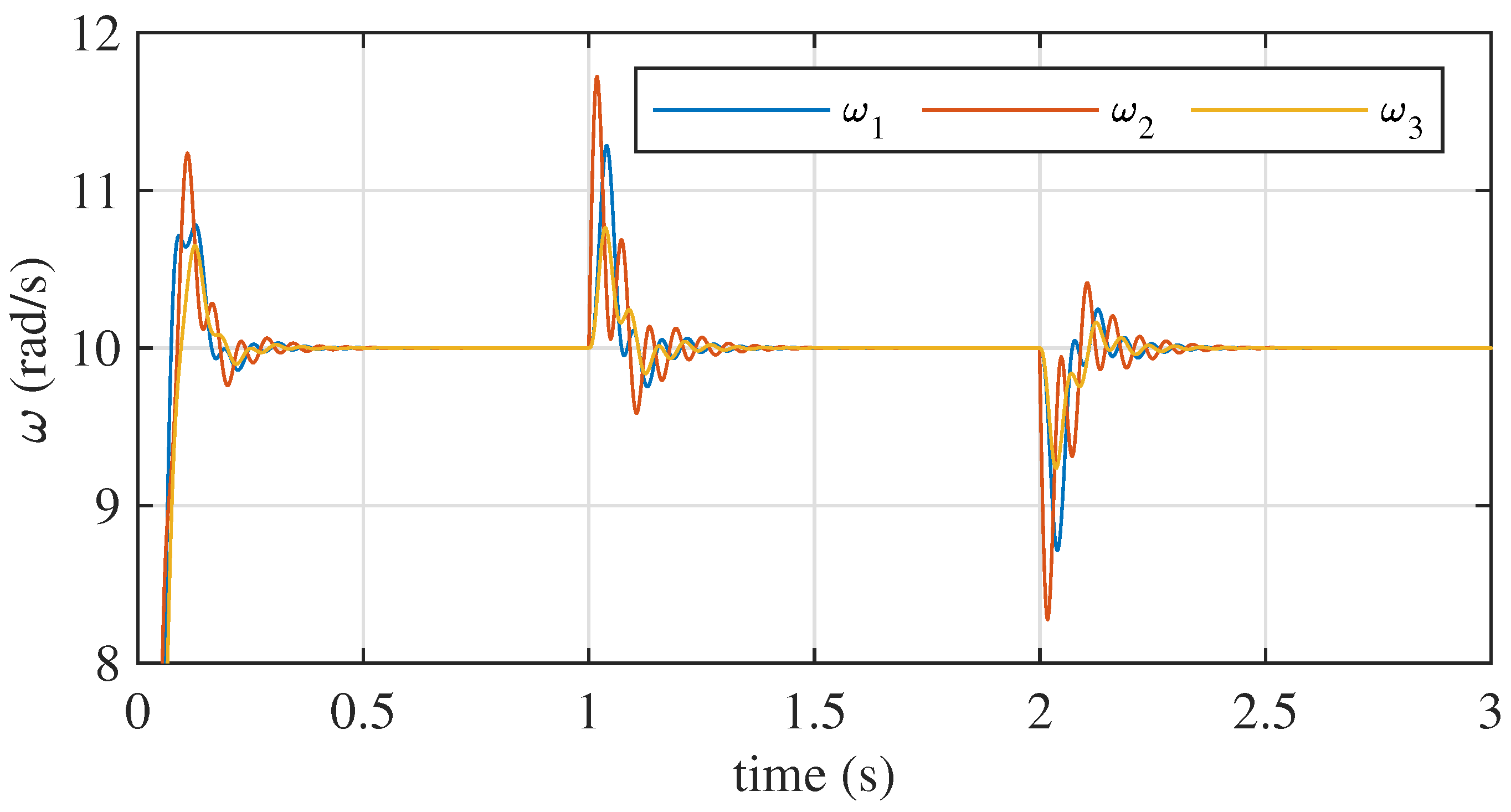
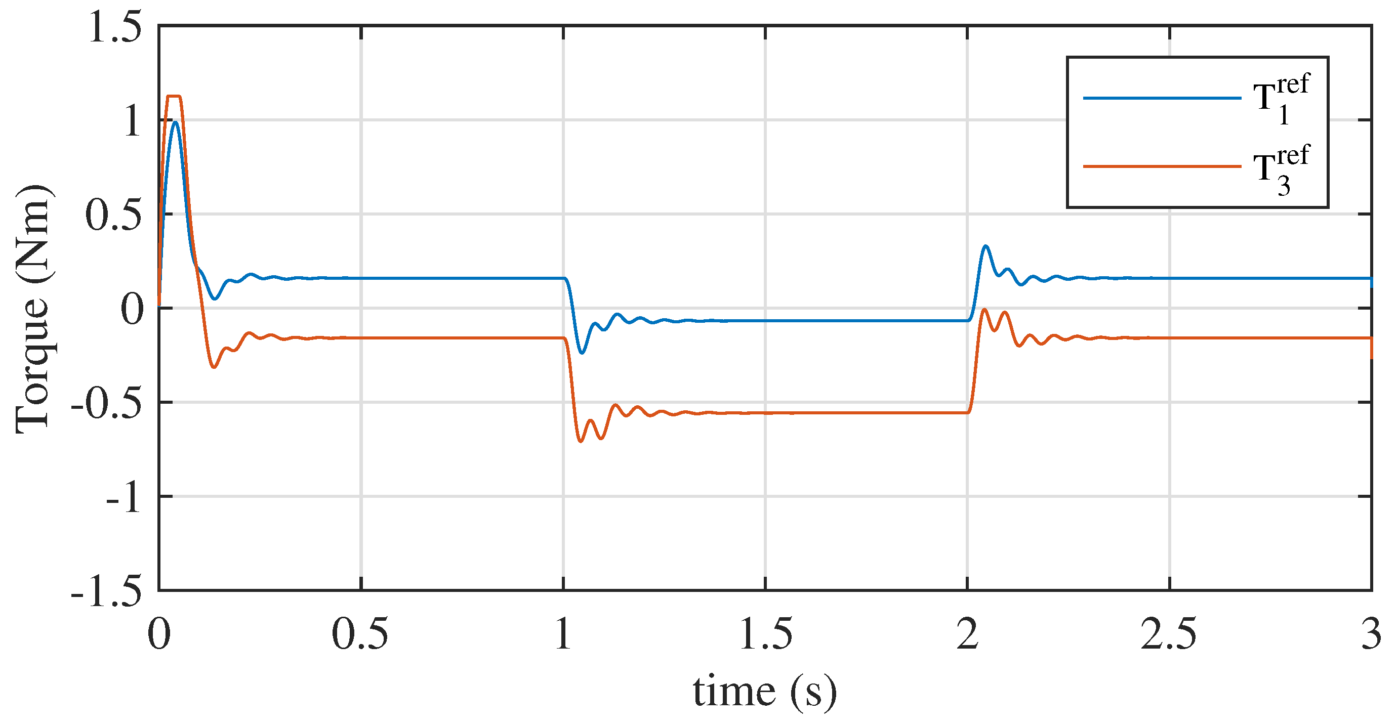
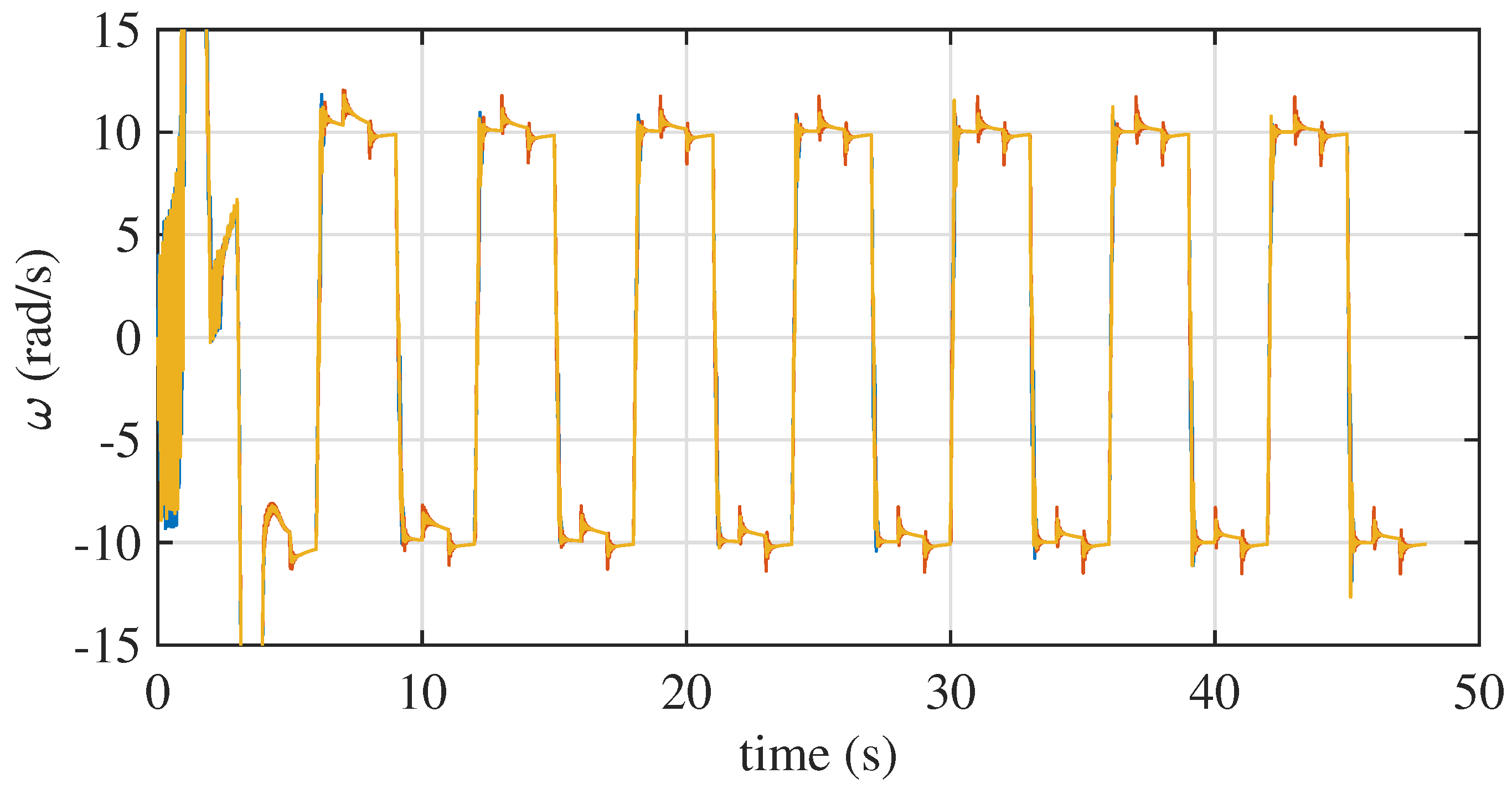
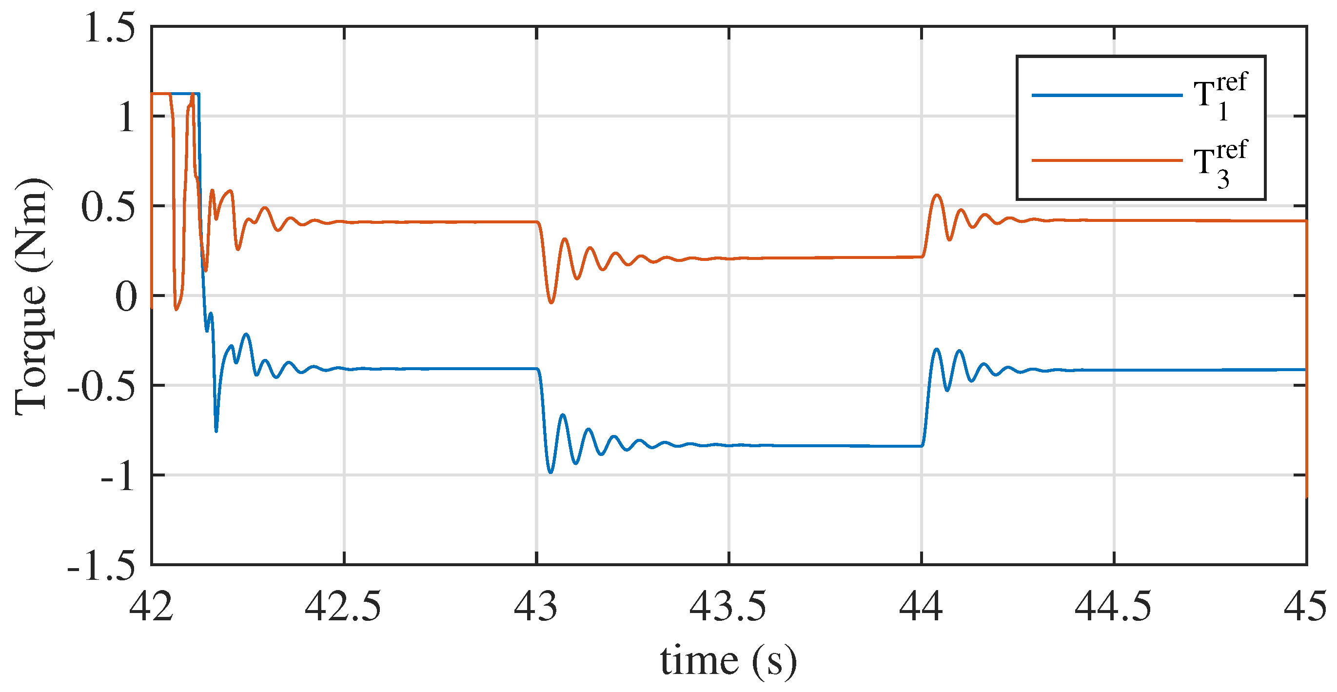
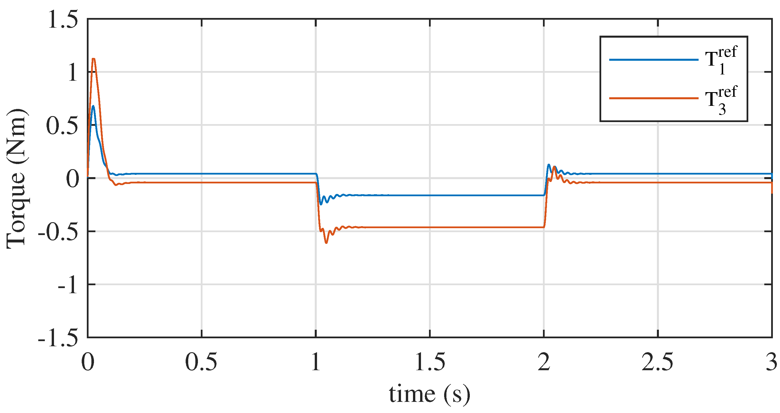
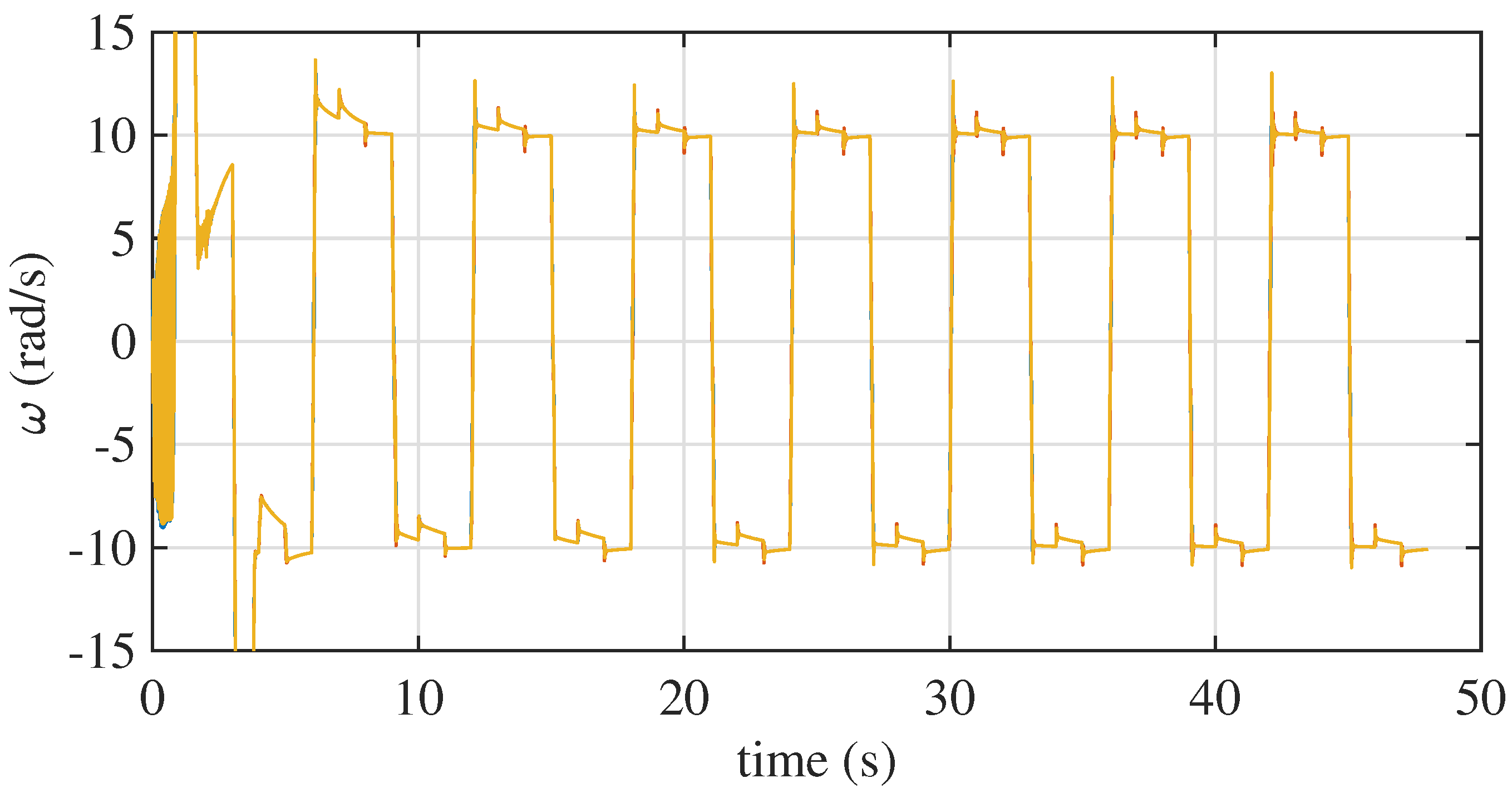
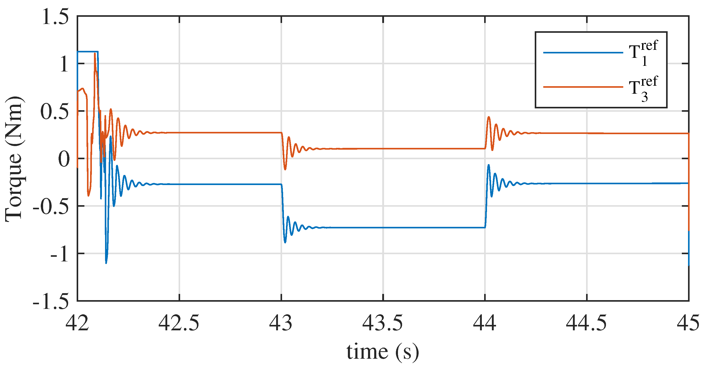
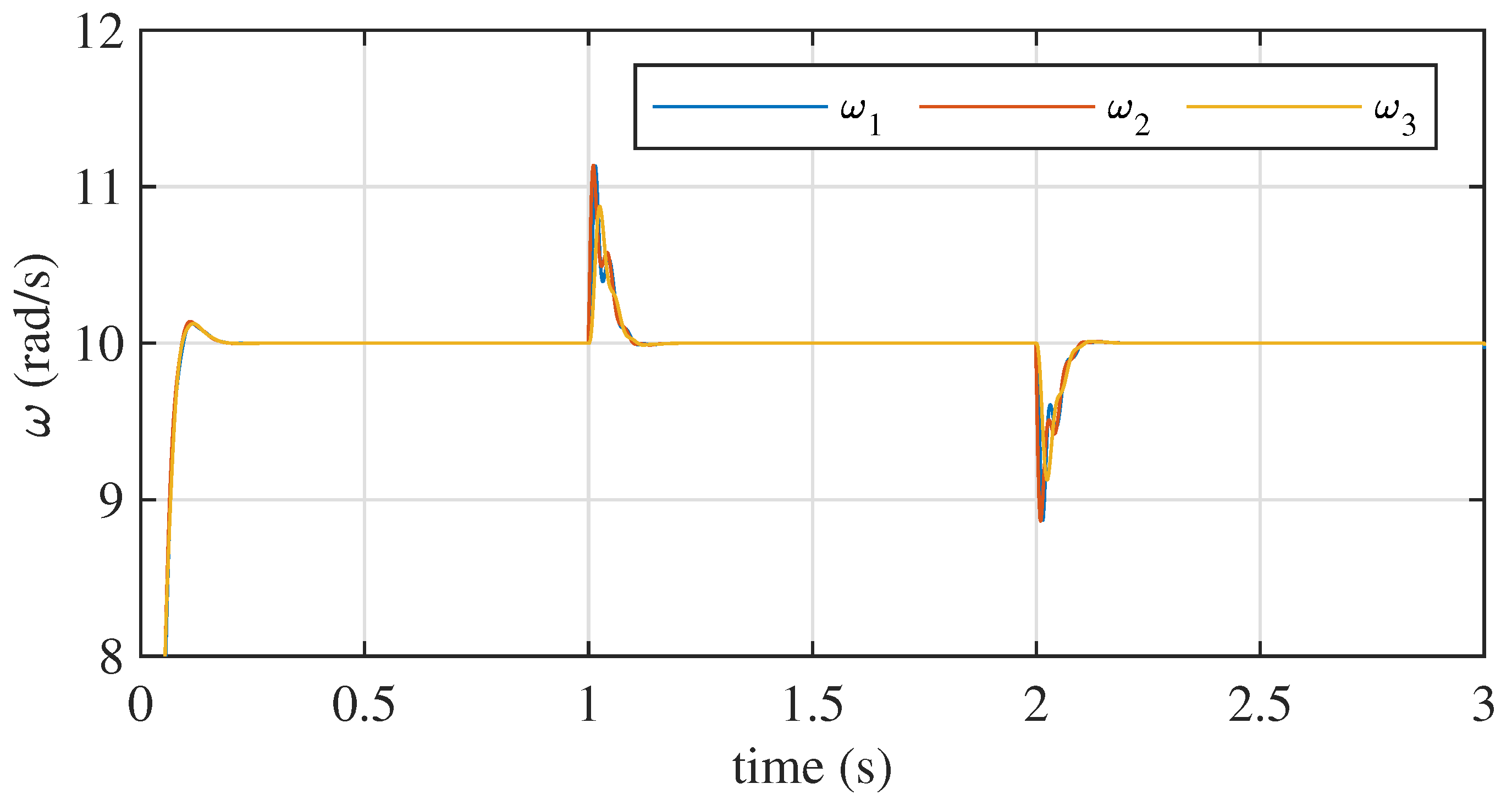
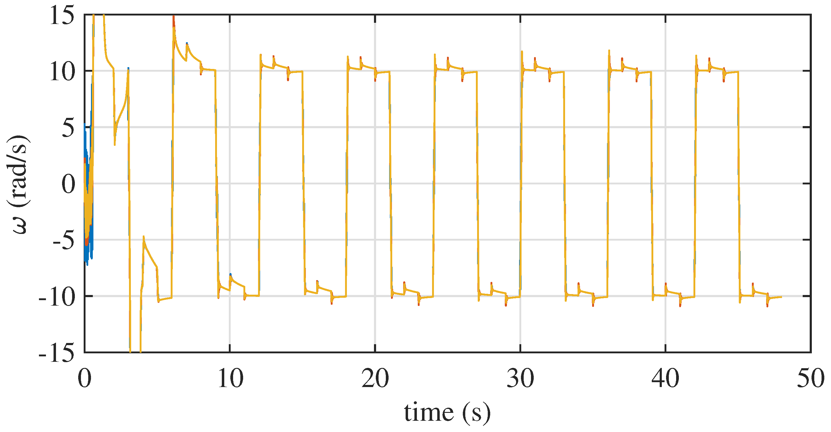
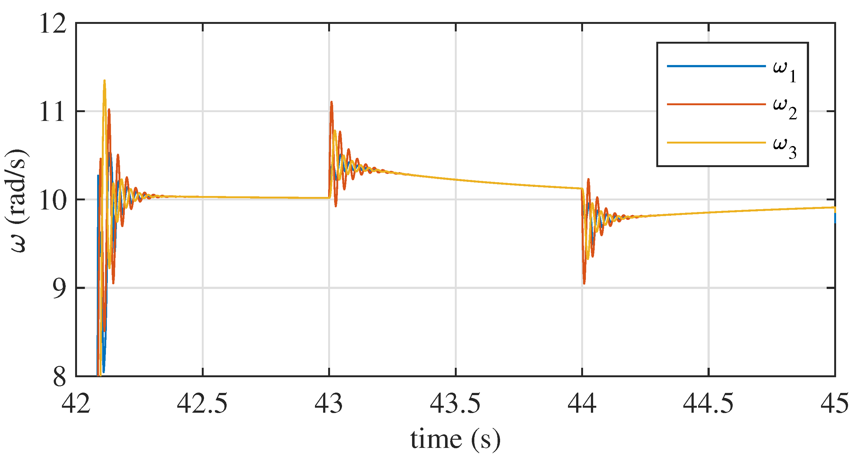
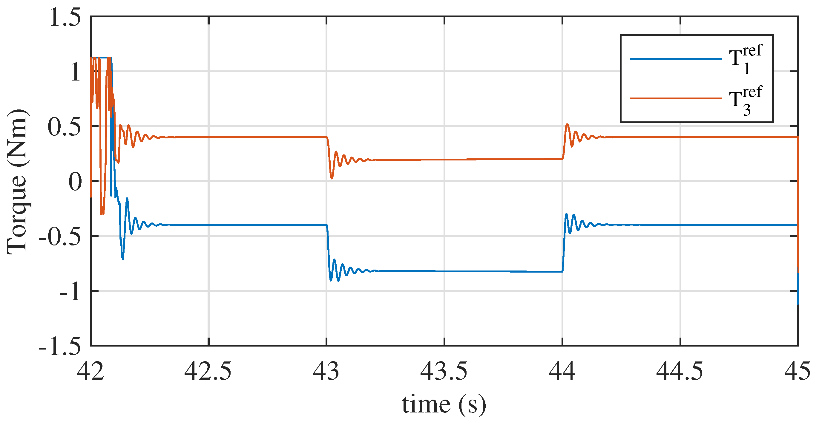
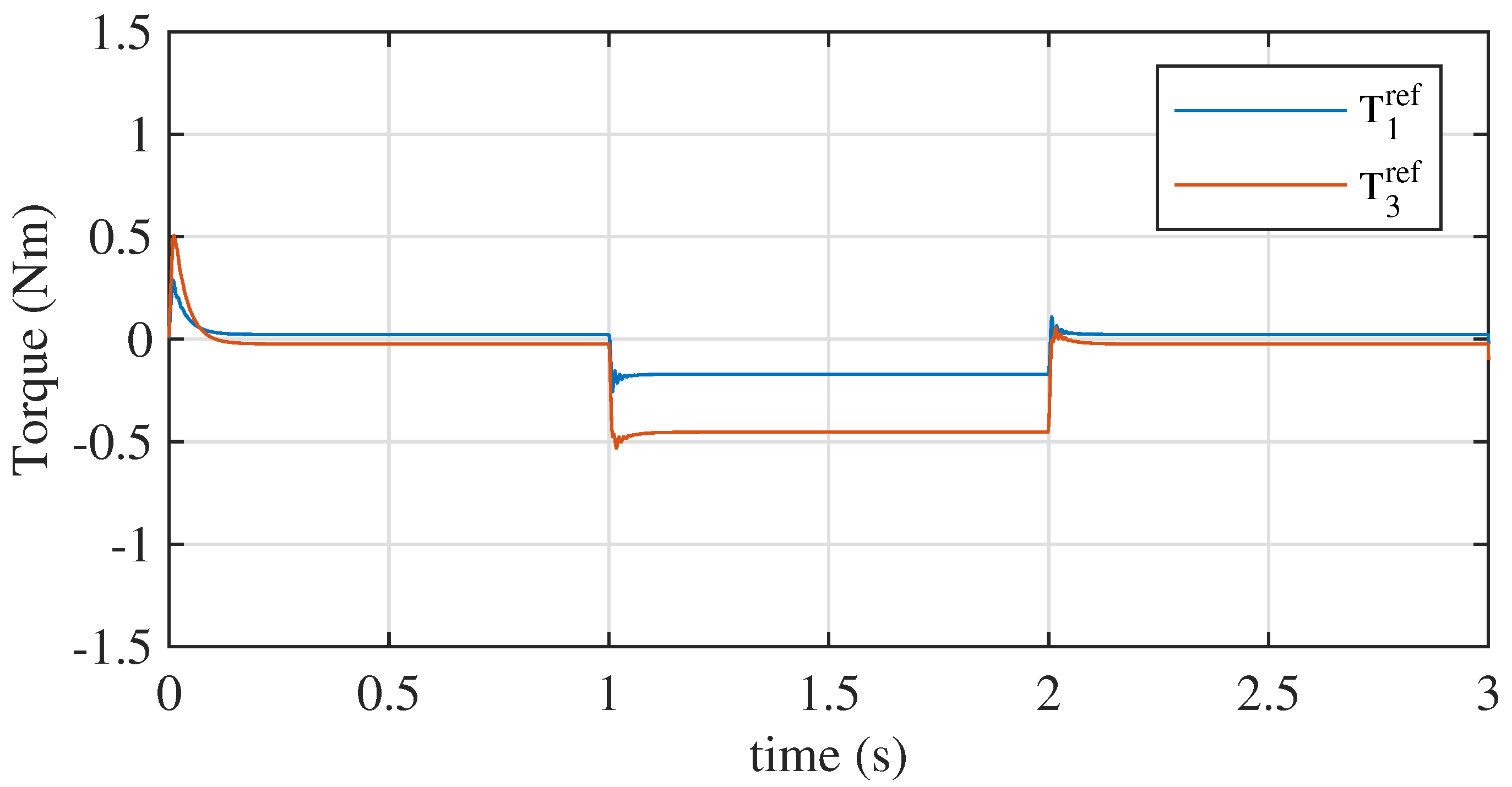
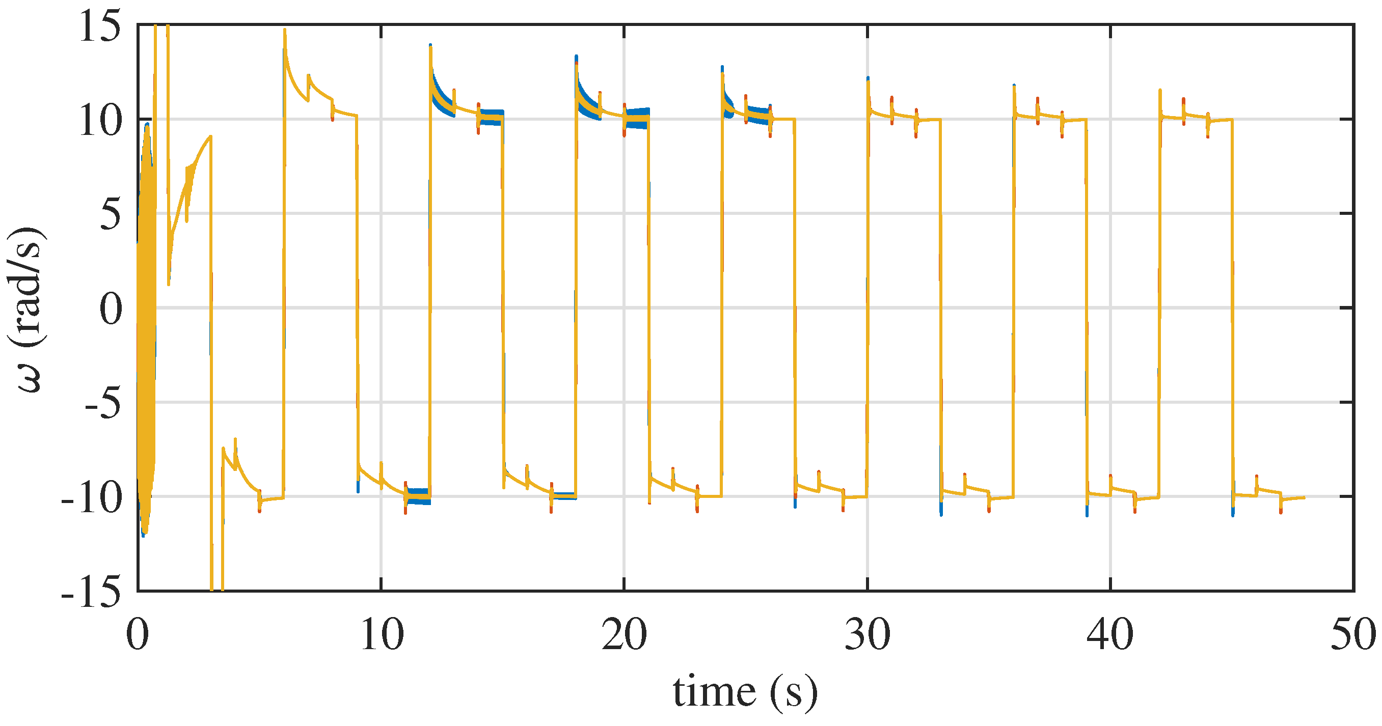
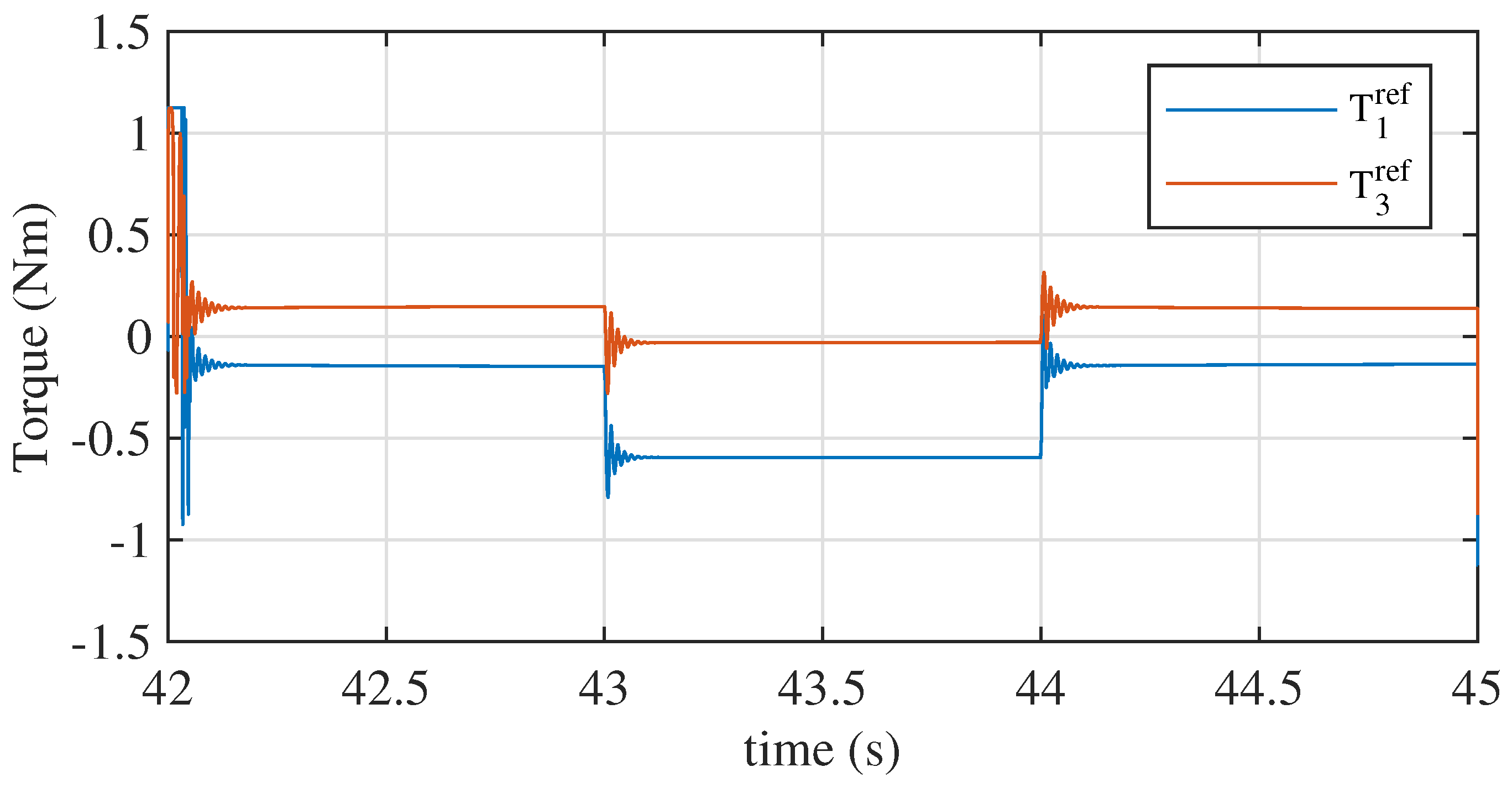
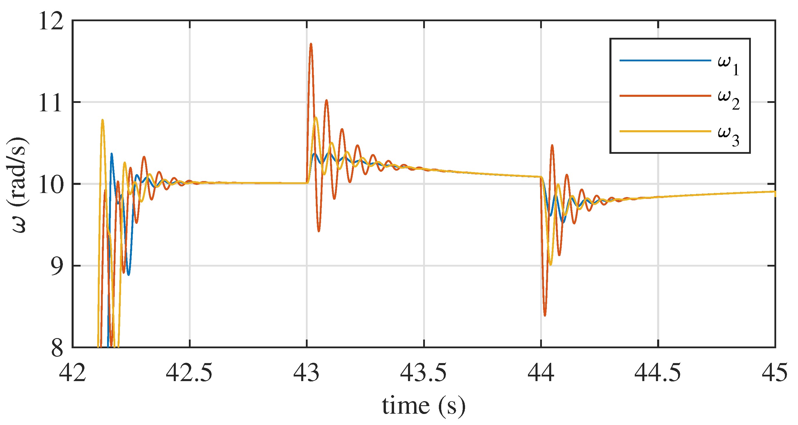
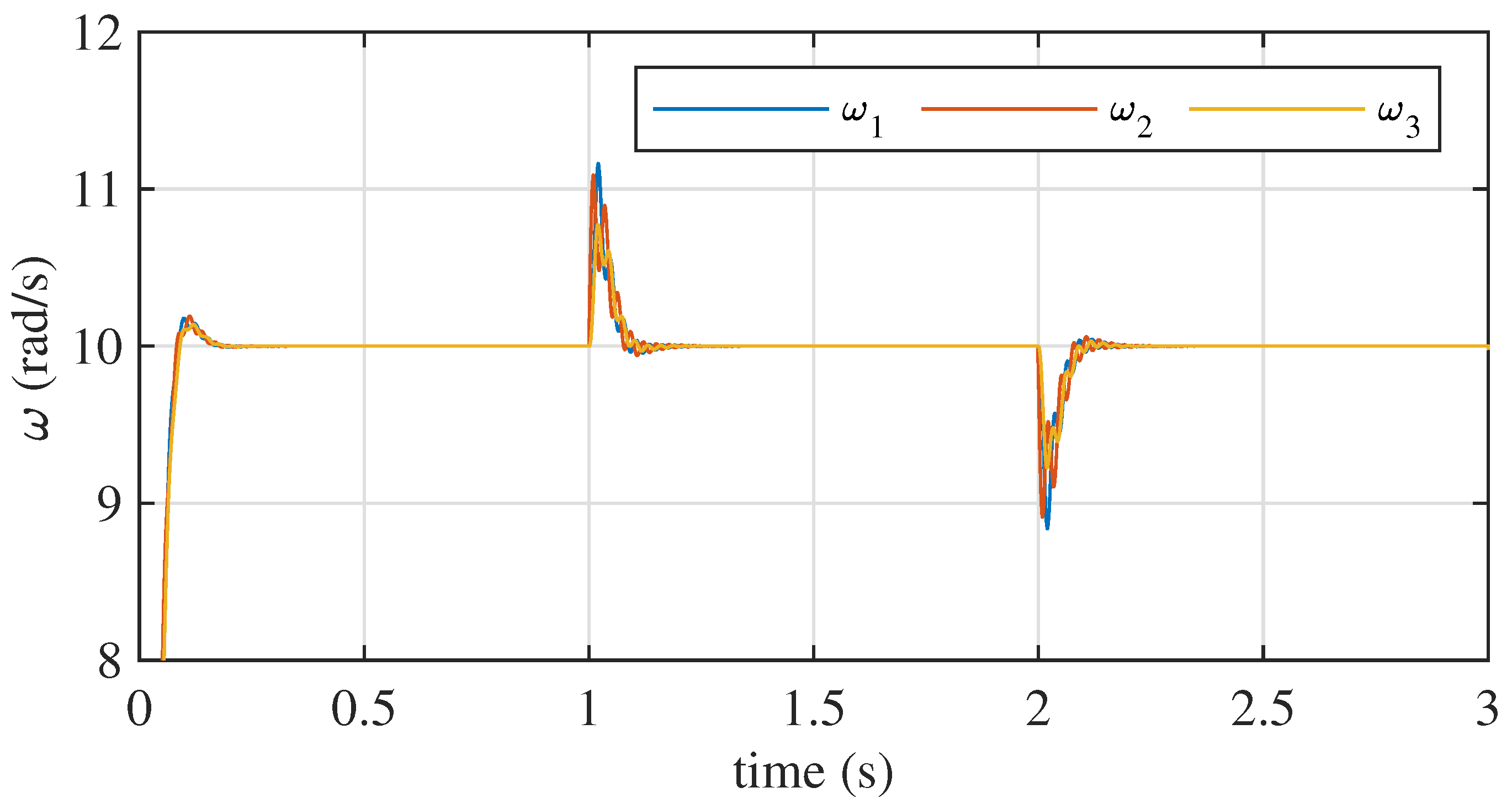
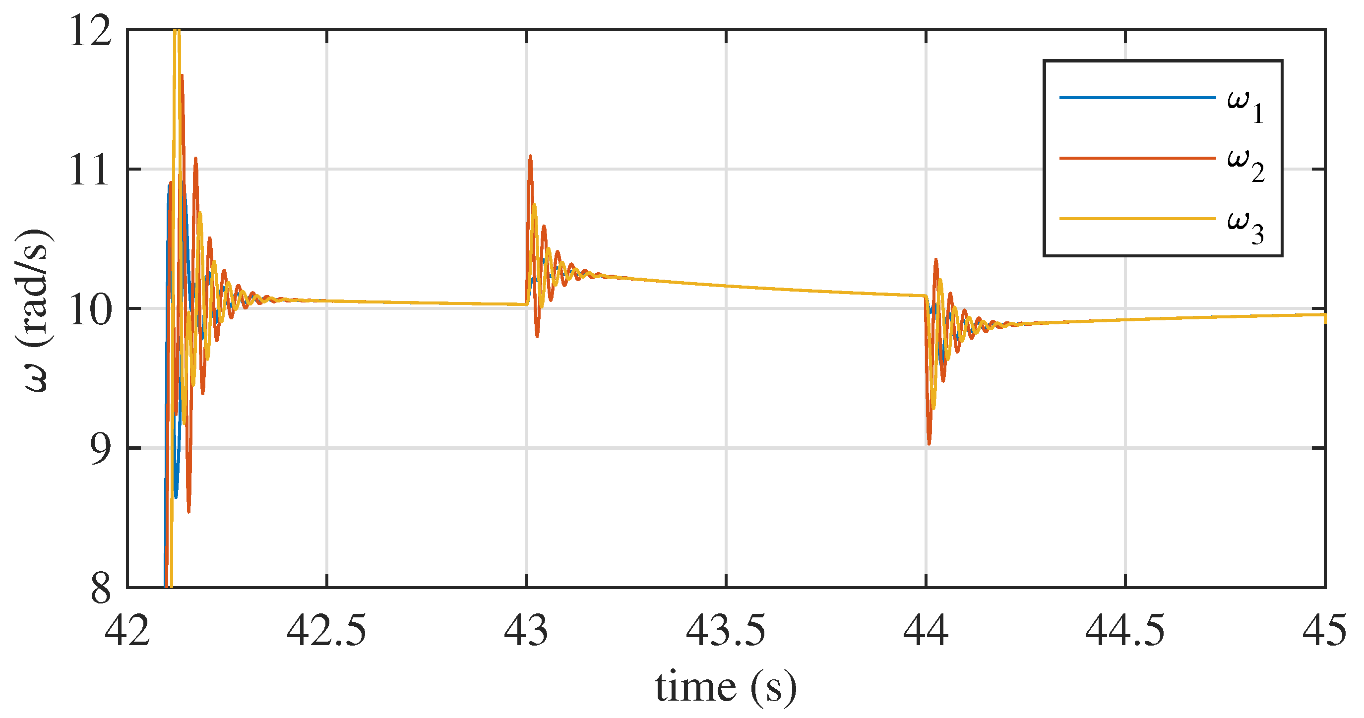
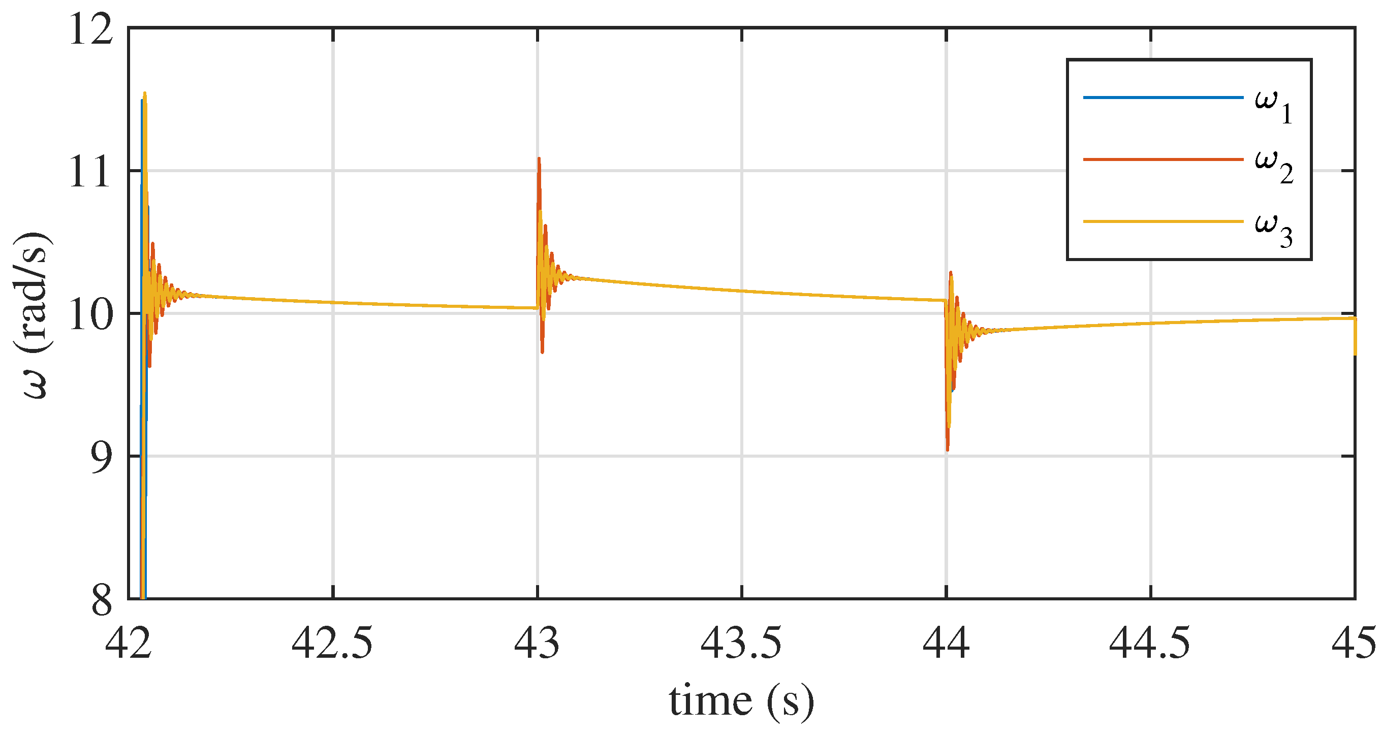
4. Results
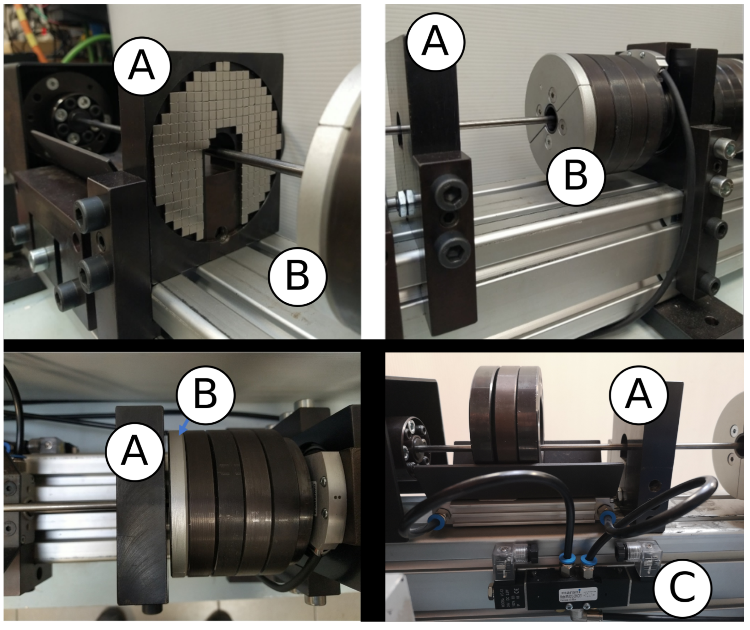
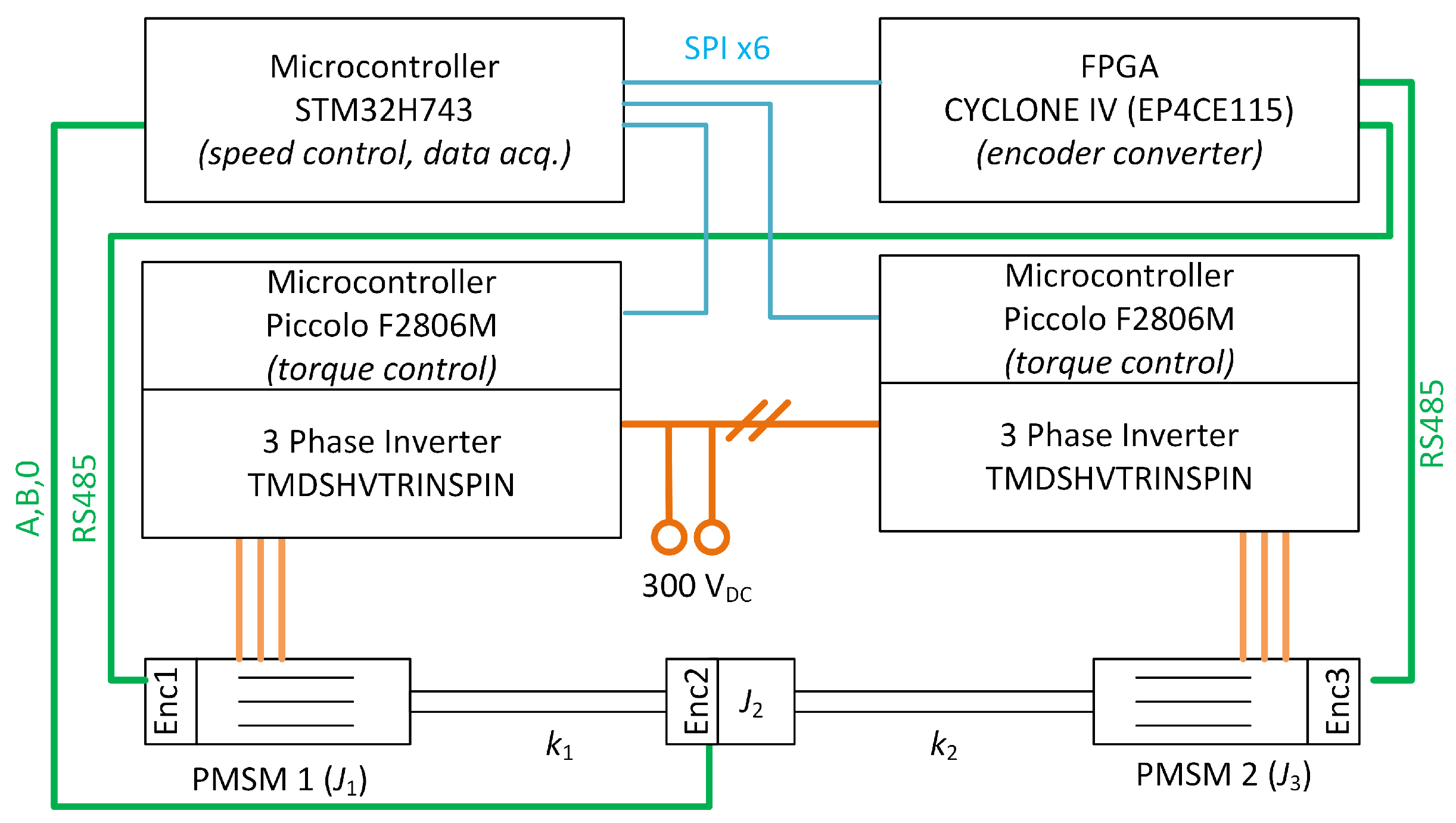
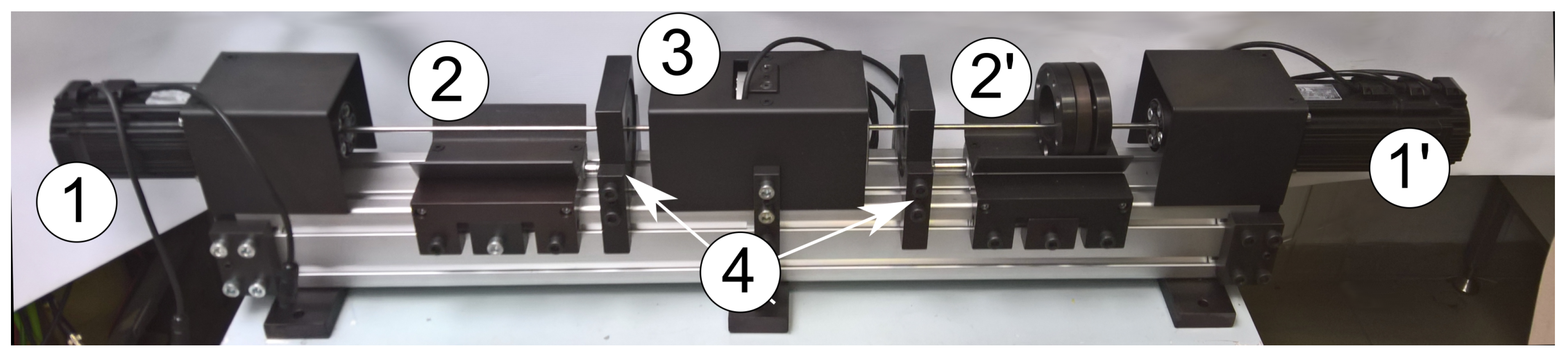
4.1. Laboratory Bench
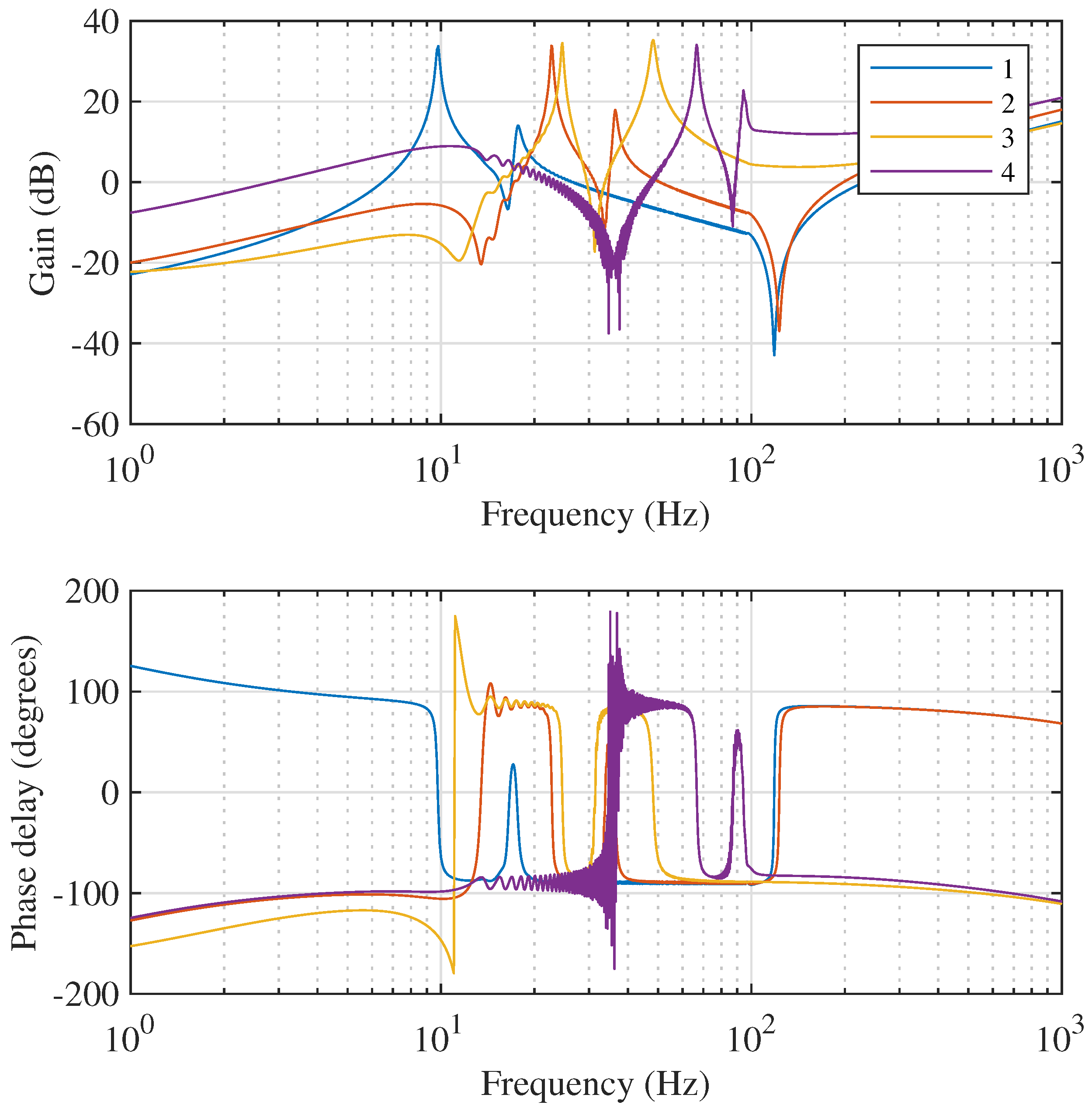
4.2. Test Configuration
- motor startup with = 10 rad/s;
- application of disturbance: load torque = 1 Nm;
- removal of disturbance: = 0 Nm;
- motor reverse, = 10 rad/s;
- application of disturbance: load torque = 1 Nm;
- removal of disturbance: = 0 Nm;
- end of test.
4.3. Comparison of Control Structures
5. Discussion
Author Contributions
Funding
Data Availability Statement
Conflicts of Interest
Abbreviations
| ANN | Artificial Neural Network |
| PMSM | Permanent Magnet Synchronous Motors |
| MLP | Multi-Layer Perceptron |
Appendix A

References
- Xia, J.; Guo, Z.; Li, Z. Optimal Online Resonance Suppression in a Drive System Based on a Multifrequency Fast Search Algorithm. IEEE Access 2021, 9, 55373–55387. [Google Scholar] [CrossRef]
- Wicher, B.; Brock, S. Comparison of Robustness of Selected Speed Control Systems Applied for Two Mass System with Backlash. In Advanced, Contemporary Control; Bartoszewicz, A., Kabzinski, J., Kacprzyk, J., Eds.; Springer International Publishing: Cham, Switzerland, 2020; pp. 1371–1382. [Google Scholar]
- Brock, S.; Łuczak, D.; Nowopolski, K.; Pajchrowski, T.; Zawirski, K. Two Approaches to Speed Control for Multi-Mass System With Variable Mechanical Parameters. IEEE Trans. Ind. Electron. 2017, 64, 3338–3347. [Google Scholar] [CrossRef]
- Luczak, D.; Wojcik, A. The study of neural estimator structure influence on the estimation quality of selected state variables of the complex mechanical part of electrical drive. In Proceedings of the 19th European Conference on Power Electronics and Applications (EPE’17 ECCE Europe), Warsaw, Poland, 11–14 September 2017. [Google Scholar]
- Li, X.; Zhou, W.; Luo, J.; Qian, J.; Ma, W.; Jiang, P.; Fan, Y. A New Mechanical Resonance Suppression Method for Large Optical Telescope by Using Nonlinear Active Disturbance Rejection Control. IEEE Access 2019, 7, 94400–94414. [Google Scholar] [CrossRef]
- Nowopolski, K.; Wicher, B.; Luczak, D.; Siwek, P. Recursive neural network as speed controller for two-sided electrical drive with complex mechanical structure. In Proceedings of the 22nd International Conference on Methods and Models in Automation and Robotics, Miedzyzdroje, Poland, 28–31 August 2017; pp. 576–581. [Google Scholar]
- Luczak, D.; Siwek, P.; Nowopolski, K. Speed Controller for Four-Mass Mechanical System with Two Drive Units. In Proceedings of the 2015 IEEE 2nd International Conference on Cybernetics (CYBCONF), Gdynia, Poland, 24–26 June 2015; pp. 449–454. [Google Scholar]
- Bobobekov, K.M. A Polynomial Method for Synthesizing a Two-Channel Regulator Stabilizing a Three-Mass System. In Proceedings of the XIV International Scientific-Technical Conference on Actual Problems of Electronics Instrument Engineering (APEIE), Novosibirsk, Russia, 2–6 October 2018; pp. 184–189. [Google Scholar]
- Hwang, S.-I.; Cho, S.-H.; Jung, J.-H.; Kim, J.-M. Phase Current Measurement Method of Dual Inverter-Motor Drive System Using a Single DC Link Current Sensor. Energies 2021, 14, 5626. [Google Scholar] [CrossRef]
- Kim, H.-W.; Amarnathvarma, A.; Kim, E.; Hwang, M.-H.; Kim, K.; Kim, H.; Choi, I.; Cha, H.-R. A Novel Torque Matching Strategy for Dual Motor-Based All-Wheel-Driving Electric Vehicles. Energies 2022, 15, 2717. [Google Scholar] [CrossRef]
- Ge, S.; Hou, S.; Yao, M. Electromechanical Coupling Dynamic Characteristics of the Dual-Motor Electric Drive System of Hybrid Electric Vehicles. Energies 2023, 16, 3190. [Google Scholar] [CrossRef]
- Nguyen, C.T.P.; Nguyen, B.-H.; Ta, M.C.; Trovão, J.P.F. Dual-Motor Dual-Source High Performance EV: A Comprehensive Review. Energies 2023, 16, 7048. [Google Scholar] [CrossRef]
- Liu, K.; Yang, P.; Wang, R.; Jiao, L.; Li, T.; Zhang, J. Observer-Based Adaptive Fuzzy Finite-Time Attitude Control for Quadrotor UAV. IEEE Trans. Aerosp. Electron. Syst. 2023, 58, 8637–8654. [Google Scholar] [CrossRef]
- Liu, K.; Yang, P.; Jiao, L.; Wang, R.; Yuan, Z.; Dong, S. Antisaturation fixed-time attitude tracking control based low-computation learning for uncertain quadrotor UAVs with external disturbances. Aerosp. Sci. Technol. 2023, 142 Pt B, 1270–9638. [Google Scholar] [CrossRef]
- Bahr, J.; Munchhof, M.; Isermann, R. Fault management for a Three Mass Torsion Oscillator. In Proceedings of the European Control Conference (ECC), Budapest, Hungary, 23–26 August 2009; pp. 3683–3688. [Google Scholar]
- Falaleev, S.; Badykov, R. Influence of turbomachinery vibration processes on the mechanical contact and dry gas seals. In Proceedings of the International Conference on Dynamics and Vibroacoustics of Machines (DVM), Samara, Russia, 16–18 September 2020; pp. 1–6. [Google Scholar]
- Melicio, R.; Mendes, V.M.F.; Catalao, J.P.S. Influence of a converter control malfunction on the harmonic behavior of wind turbines with permanent magnet generator. In Proceedings of the IEEE International Electric Machines & Drives Conference (IEMDC), Niagara Falls, ON, Canada, 15–18 May 2011; pp. 783–788. [Google Scholar]
- Cai, J.; Wang, J.; Zhang, J.; Weng, H. Study on Torsional Vibration Characteristics of Wind Turbine Drive Train. In Proceedings of the 5th International Conference on Energy, Electrical and Power Engineering (CEEPE), Chongqing, China, 22–24 April 2022; pp. 927–931. [Google Scholar]
- Li, H.; Chen, Z. Transient Stability Analysis of Wind Turbines with Induction Generators Considering Blades and Shaft Flexibility. In Proceedings of the IECON—33rd Annual Conference of the IEEE Industrial Electronics Society, Taipei, Taiwan, 5–8 November 2007; pp. 1604–1609. [Google Scholar]
- Han, X.; Wang, P.; Wang, P.; Qin, W. Transient stability studies of doubly-fed induction generator using different drive train models. In Proceedings of the IEEE Power and Energy Society General Meeting, Detroit, MI, USA, 24–28 July 2011. [Google Scholar]
- Qiu, J.J.; Ta, N. Multiple resonance of coupled lateral and torsional vibration excited by electromagnetic forces on rotor shaft system of generators. In Proceedings of the International Conference on Power System Technology, Kunming, China, 13–17 October 2002; pp. 2193–2197. [Google Scholar]
- Takeichi, Y.; Komada, S.; Ishida, M.; Hori, T. Speed control of symmetrical type three-mass resonant system by PID-controller. In Proceedings of the 4th IEEE International Workshop on Advanced Motion Control-AMC ’96-MIE, Mie, Japan, 18–21 March 1996; pp. 594–599. [Google Scholar]
- Kuznetsov, B.; Bovdui, I.; Nikitina, T.; Kolomiets, V.; Kobylianskyi, B. Multiobjective Parametric Synthesis of Robust Control by Rolling Mills Main Electric Drives. In Proceedings of the IEEE Problems of Automated Electrodrive. Theory and Practice (PAEP), Kremenchuk, Ukraine, 21–25 September 2020. [Google Scholar]
- Valenzuela, M.A.; Bentley, J.M.; Lorenz, R.D. Evaluation of torsional oscillations in paper machine sections. IEEE Trans. Ind. Appl. 2005, 41, 493–501. [Google Scholar] [CrossRef]
- Kwon, Y.S.; Hwang H., W.; Choi, Y.S. Stabilization loop design on direct drive gimbaled platform with low stiffness and heavy inertia. In Proceedings of the International Conference on Control, Automation and Systems, Seoul, Republic of Korea, 17–20 October 2007; pp. 320–325. [Google Scholar]
- Luczak, D. Mathematical Model of Multi-Mass Electric Drive System with Flexible Connection. In Proceedings of the 19th International Conference on Methods and Models in Automation and Robotics (MMAR), Miedzyzdroje, Poland, 2–5 September 2014; pp. 590–595. [Google Scholar]
- Torikai, K.; Katsura, S. Position control of 2-DOF resonant system based on modal-space control design. In Proceedings of the IEEE International Conference on Industrial Technology (ICIT), Lyon, France, 20–22 February 2018; pp. 286–291. [Google Scholar]
- Cychowski, M.; Jaskiewicz, R.; Szabat, K. Model Predictive Control of an elastic three-mass drive system with torque constraints. In Proceedings of the IEEE International Conference on Industrial Technology, Via del Mar, Chile, 14–17 March 2010; pp. 379–385. [Google Scholar]
- Saito, E.; Katsura, S. Vibration suppression of resonant system by using wave compensator. In Proceedings of the IECON—37th Annual Conference of the IEEE Industrial Electronics Society, Melbourne, VIC, Australia, 7–10 November 2011; pp. 4250–4255. [Google Scholar]
- Luczak, D.; Nowopolski, K. Identification of Multi-Mass Mechanical Systems in Electrical Drives. In Proceedings of the 2014 16th International Conference on Mechatronics—Mechatronika (ME), Brno, Czech Republic, 3–5 December 2014; pp. 275–282. [Google Scholar]
- Eker, I.; Vural, M. Experimental online identification of a three-mass mechanical system. In Proceedings of the IEEE Conference on Control Applications, Istanbul, Turkey, 25–25 June 2003; pp. 60–65. [Google Scholar]
- Villwock, S.; Pacas, M. Application of the Welch-Method for the Identification of Two- and Three-Mass-Systems. IEEE Trans. Ind. Electron. 2008, 55, 457–466. [Google Scholar] [CrossRef]
- Zawirski, K.; Nowopolski, K.; Siwek, P. Application of Cuckoo Search Algorithm for Speed Control Optimization in Two-Sided Electrical Drive. In Proceedings of the IEEE 18th International Power Electronics and Motion Control Conference (PEMC), Budapest, Hungary, 26–30 August 2018; pp. 651–656. [Google Scholar]
- Yang, X.S.; Suash, D. Cuckoo Search via Lévy flights. In Proceedings of the World Congress on Nature & Biologically Inspired Computing (NaBIC), Coimbatore, India, 9–11 December 2009; pp. 210–214. [Google Scholar]
- Pajchrowski, T.; Siwek, P.; Wojcik, A. Application of the Reinforcement Learning method for adaptive electric drive control with variable parameters. In Proceedings of the IEEE 19th International Power Electronics and Motion Control Conference (PEMC), Gliwice, Poland, 25–29 April 2021; pp. 687–694. [Google Scholar]
- Caponetto, R.; Fortuna, L.; Porto, D. Parameter tuning of a non integer order PID controller. In Proceedings of the 15th International Symposium on Mathematical Theory of Networks and Systems, Notre Dame, Indiana, 12–16 August 2002. [Google Scholar]
- Arena, P.; Fortuna, L.; Occhipinti, L.; Xibilia, M.G. Neural networks for quaternion-valued function approximation. In Proceedings of the IEEE International Symposium on Circuits and Systems—ISCAS ’94, London, UK, 30 May 1994–2 June 1994; Volume 6, pp. 307–310. [Google Scholar] [CrossRef]


| Parameter Name | Value for Conf. 1 | Value for Conf. 2 | Value for Conf. 3 | Value for Conf. 4 | Unit |
|---|---|---|---|---|---|
| Number of discs on motor 1 side | 6 | 3 | 0 | 0 | - |
| Number of discs on intermediate mass | 4 | 3 | 3 | 0 | - |
| Number of discs on motor 2 side | 6 | 3 | 6 | 0 | - |
| Moment of inertia | 7.2 | 4.2 | 1.2 | 1.2 | |
| Moment of inertia | 6.4 | 5.4 | 5.4 | 2.4 | |
| Moment of inertia | 7.2 | 4.2 | 7.2 | 1.2 | |
| Diameter of the shaft | 6 | 8 | 8 | 10 | mm |
| Stiffness of the shaft | 27.1 | 85.5 | 85.5 | 208.8 | Nm/rad |
| Mechanical resonance | 9.8 | 22.7 | 24.6 | 66.7 | Hz |
| Mechanical resonance | 17.6 | 36.3 | 48.2 | 94.3 | Hz |
| Response Type | Signal | Controller | Overshoot (%) | Undersh. (%) | |||||||
|---|---|---|---|---|---|---|---|---|---|---|---|
| Comm. | PI | 0.475676 | 0.018188 | 0.001610 | 3.142198 | 0.065218 | 0.002309 | 0.154800 | 7.799524 | 1.397745 | |
| ANN | 1.469595 | 0.091754 | 0.012745 | 17.108191 | 0.620226 | 0.040962 | 0.260700 | 3.704077 | 11.152766 | ||
| PI | 0.481832 | 0.019172 | 0.001970 | 3.314993 | 0.065401 | 0.002233 | 0.205700 | 12.360894 | 2.374302 | ||
| ANN | 1.450212 | 0.088613 | 0.013224 | 17.797861 | 0.597070 | 0.035857 | 0.314800 | 3.309337 | 10.888808 | ||
| PI | 0.450904 | 0.016901 | 0.001393 | 2.761537 | 0.057830 | 0.002120 | 0.154800 | 6.490114 | 1.022262 | ||
| ANN | 1.434597 | 0.085141 | 0.011761 | 17.664204 | 0.656812 | 0.040898 | 0.298500 | 7.847255 | 22.912434 | ||
| Disturb. | PI | 0.058514 | 0.004119 | 0.000572 | 0.044306 | 0.001910 | 0.000102 | 0.137300 | 12.848921 | 2.458527 | |
| ANN | 0.188302 | 0.074224 | 0.042927 | 0.041612 | 0.012643 | 0.006120 | 0.429800 | 3.778754 | 0.000000 | ||
| PI | 0.085405 | 0.006166 | 0.001041 | 0.072539 | 0.002327 | 0.000155 | 0.164400 | 17.229900 | 4.143409 | ||
| ANN | 0.236961 | 0.076389 | 0.043256 | 0.119628 | 0.016301 | 0.006538 | 0.482600 | 17.141712 | 5.829159 | ||
| PI | 0.042534 | 0.003134 | 0.000424 | 0.017494 | 0.000796 | 0.000048 | 0.097000 | 7.634733 | 1.628954 | ||
| ANN | 0.202230 | 0.075590 | 0.043484 | 0.056523 | 0.013624 | 0.006323 | 0.447200 | 8.133003 | 0.000000 |
| Response Type | Signal | Controller | Overshoot (%) | Undersh. (%) | |||||||
|---|---|---|---|---|---|---|---|---|---|---|---|
| Comm. | PI | 0.366910 | 0.009129 | 0.000411 | 2.550049 | 0.041573 | 0.001066 | 0.079400 | 1.777378 | 0.065308 | |
| ANN | 1.159534 | 0.067884 | 0.016721 | 13.978417 | 0.405992 | 0.020315 | 0.208600 | 9.093898 | 13.536801 | ||
| PI | 0.367358 | 0.009088 | 0.000411 | 2.572995 | 0.041187 | 0.001052 | 0.078100 | 1.905039 | 0.072693 | ||
| ANN | 1.192442 | 0.072759 | 0.017689 | 14.227942 | 0.396247 | 0.019711 | 0.247300 | 16.713779 | 14.590303 | ||
| PI | 0.366135 | 0.009511 | 0.000436 | 2.402996 | 0.040958 | 0.001131 | 0.083600 | 1.383679 | 0.040539 | ||
| ANN | 1.199338 | 0.072890 | 0.017531 | 14.202800 | 0.403441 | 0.020049 | 0.223500 | 30.165049 | 8.232933 | ||
| Disturb. | PI | 0.038624 | 0.001484 | 0.000091 | 0.025460 | 0.000702 | 0.000024 | 0.059400 | 11.625402 | 0.440067 | |
| ANN | 0.168603 | 0.069530 | 0.041595 | 0.031590 | 0.010509 | 0.005507 | 0.319200 | 3.523109 | 0.000000 | ||
| PI | 0.043004 | 0.001629 | 0.000185 | 0.027838 | 0.000695 | 0.000034 | 0.070100 | 10.884656 | 1.665872 | ||
| ANN | 0.179785 | 0.069617 | 0.041562 | 0.045032 | 0.010722 | 0.005512 | 0.321000 | 10.939501 | 2.014208 | ||
| PI | 0.033590 | 0.001359 | 0.000081 | 0.016916 | 0.000544 | 0.000021 | 0.059600 | 7.748143 | 0.316555 | ||
| ANN | 0.174003 | 0.069638 | 0.041620 | 0.037511 | 0.010643 | 0.005517 | 0.319100 | 7.485419 | 0.000000 |
| Response Type | Signal | Controller | Overshoot (%) | Undersh. (%) | |||||||
|---|---|---|---|---|---|---|---|---|---|---|---|
| Comm. | PI | 0.368796 | 0.009580 | 0.000441 | 2.444216 | 0.041375 | 0.001130 | 0.084000 | 1.294777 | 0.016356 | |
| ANN | 1.037062 | 0.051715 | 0.010257 | 12.470511 | 0.341269 | 0.015544 | 0.170800 | 5.273403 | 19.552395 | ||
| PI | 0.371152 | 0.009373 | 0.000426 | 2.560503 | 0.041567 | 0.001092 | 0.082100 | 1.384340 | 0.017960 | ||
| ANN | 1.046081 | 0.051978 | 0.010432 | 12.704889 | 0.322951 | 0.014224 | 0.204200 | 10.205833 | 14.884428 | ||
| PI | 0.371601 | 0.009617 | 0.000440 | 2.487840 | 0.042119 | 0.001150 | 0.082900 | 1.256414 | 0.017973 | ||
| ANN | 1.034782 | 0.049752 | 0.010044 | 12.662521 | 0.313893 | 0.013143 | 0.182800 | 13.500639 | 7.773084 | ||
| Disturb. | PI | 0.037192 | 0.001297 | 0.000068 | 0.022974 | 0.000582 | 0.000020 | 0.063100 | 11.319983 | 0.111228 | |
| ANN | 0.235775 | 0.096195 | 0.057317 | 0.062348 | 0.020240 | 0.010500 | 0.597300 | 5.100484 | 0.0000000 | ||
| PI | 0.041123 | 0.001379 | 0.000149 | 0.026829 | 0.000604 | 0.000030 | 0.061500 | 11.366243 | 1.665878 | ||
| ANN | 0.244301 | 0.096267 | 0.057291 | 0.076086 | 0.020523 | 0.010516 | 0.597900 | 11.070268 | 0.772131 | ||
| PI | 0.033103 | 0.001285 | 0.000068 | 0.017971 | 0.000558 | 0.000020 | 0.068600 | 8.744784 | 0.122135 | ||
| ANN | 0.240040 | 0.096426 | 0.057407 | 0.067576 | 0.020415 | 0.010535 | 0.598600 | 7.815338 | 0.000000 |
| Response Type | Signal | Controller | Overshoot (%) | Undersh. (%) | |||||||
|---|---|---|---|---|---|---|---|---|---|---|---|
| Comm. | PI | 0.348451 | 0.010413 | 0.000610 | 2.005618 | 0.031441 | 0.000930 | 0.120100 | 0.000000 | 0.000000 | |
| ANN | 0.429887 | 0.036262 | 0.018493 | 4.360812 | 0.043603 | 0.001786 | 0.071400 | 14.884961 | 20.404839 | ||
| PI | 0.348626 | 0.010402 | 0.000609 | 2.012884 | 0.031383 | 0.000928 | 0.120100 | 0.000000 | 0.000000 | ||
| ANN | 0.430648 | 0.036185 | 0.018508 | 4.498573 | 0.041529 | 0.001713 | 0.092300 | 8.486324 | 3.726196 | ||
| PI | 0.348800 | 0.010504 | 0.000616 | 1.985768 | 0.031714 | 0.000947 | 0.120400 | 0.000000 | 0.000000 | ||
| ANN | 0.436971 | 0.036434 | 0.018528 | 4.519956 | 0.043908 | 0.001760 | 0.093600 | 15.430262 | 1.817590 | ||
| Disturb. | PI | 0.034560 | 0.001145 | 0.000069 | 0.020327 | 0.000380 | 0.000011 | 0.055400 | 13.045721 | 0.073611 | |
| ANN | 0.163573 | 0.067318 | 0.040436 | 0.029538 | 0.009790 | 0.005181 | 0.279900 | 3.409328 | 0.000000 | ||
| PI | 0.036229 | 0.001329 | 0.000254 | 0.020725 | 0.000420 | 0.000060 | 0.055900 | 10.912074 | 3.708754 | ||
| ANN | 0.168881 | 0.067390 | 0.040478 | 0.035679 | 0.009856 | 0.005198 | 0.280000 | 10.835793 | 2.782432 | ||
| PI | 0.032739 | 0.001142 | 0.000070 | 0.016515 | 0.000356 | 0.000011 | 0.055700 | 8.743014 | 0.071546 | ||
| ANN | 0.165811 | 0.067342 | 0.040443 | 0.031936 | 0.009817 | 0.005183 | 0.280100 | 7.146510 | 0.442697 |
Disclaimer/Publisher’s Note: The statements, opinions and data contained in all publications are solely those of the individual author(s) and contributor(s) and not of MDPI and/or the editor(s). MDPI and/or the editor(s) disclaim responsibility for any injury to people or property resulting from any ideas, methods, instructions or products referred to in the content. |
© 2023 by the authors. Licensee MDPI, Basel, Switzerland. This article is an open access article distributed under the terms and conditions of the Creative Commons Attribution (CC BY) license (https://creativecommons.org/licenses/by/4.0/).
Share and Cite
Zawirski, K.; Brock, S.; Nowopolski, K. Recursive Neural Network as a Multiple Input–Multiple Output Speed Controller for Electrical Drive of Three-Mass System. Energies 2024, 17, 172. https://doi.org/10.3390/en17010172
Zawirski K, Brock S, Nowopolski K. Recursive Neural Network as a Multiple Input–Multiple Output Speed Controller for Electrical Drive of Three-Mass System. Energies. 2024; 17(1):172. https://doi.org/10.3390/en17010172
Chicago/Turabian StyleZawirski, Krzysztof, Stefan Brock, and Krzysztof Nowopolski. 2024. "Recursive Neural Network as a Multiple Input–Multiple Output Speed Controller for Electrical Drive of Three-Mass System" Energies 17, no. 1: 172. https://doi.org/10.3390/en17010172
APA StyleZawirski, K., Brock, S., & Nowopolski, K. (2024). Recursive Neural Network as a Multiple Input–Multiple Output Speed Controller for Electrical Drive of Three-Mass System. Energies, 17(1), 172. https://doi.org/10.3390/en17010172