A Study and Optimization of the Unsteady Flow Characteristics in the Last Stage Impeller of a Small-Scale Multi-Stage Hydraulic Turbine

Abstract

The demand for small-size multi-stage hydraulic turbines is experiencing rapid growth due to the ongoing efforts towards energy conservation and emission reduction. On account of their compact structural design, these turbines feature a more intricate internal flow configuration, rendering them prone to the creation of low-pressure zones, resulting in vapor–liquid two-phase flow, accompanied by the development of intense vibrations and noise, thereby adversely affecting the safety and stability of turbine operations. Concurrently, an innovative method for analyzing flow fields has been formulated combined with two-dimensional frequency domain visualization technology and proper orthogonal decomposition, serving to establish a diagnostic and optimization framework for the unsteady flow structures within rotating machinery by considering the features related to frequency distribution, spatial distribution, and energy contributions. It was found that there are two main unsteady flow structures which are the areas with high risks of vaporization under this study condition. According to the flow characteristics of the analysis, an optimization scheme was proposed to improve the two-phase flow problem in the secondary impeller, and the preliminary results were satisfactory.

1. Introduction

Considering the advancing global energy revolution, an increasing consensus has emerged regarding the necessity for the advancement of low-carbon and clean energy development. This shift not only presents significant opportunities but also entails formidable challenges for the advancement of energy storage and recycling technology [1]. In comparison to other energy storage technologies, pumped storage stands out as the most mature and versatile green energy storage method, boasting discernible economic advantages [2]. Pumped storage technology is an important means of energy storage and transformation. It has strong adjustment ability, flexibility, high efficiency, mature technology, low development cost, long service life, and can store unstable tidal energy and offshore wind energy. It is of great significance to the stable operation of the power grid and the stable supply of energy [3].

Simultaneously, there is a growing focus on small and micro-pumped storage systems attributed to their compact installation, minimal water requisites, and adaptable site layout [4]. These inherent attributes bestow upon them promising prospects for application across various industries, particularly in the realms of energy recovery and small-scale energy storage [5]. Currently, the design parameters for small multi-stage hydraulic turbines are progressing towards heightened levels of compactness and efficiency. The inherent complexity of the internal flow within a small-scale multi-stage hydraulic turbine is noteworthy, and cavitation is one of them.

Cavitation is a unique physical property of liquid due to local pressure drops to saturated vapor pressure; the continuity of water is destroyed to form bubbles, which includes inception, growth, contraction, and ultimate collapse [6,7]. Cavitation in a hydraulic turbine involves a transition from single-phase liquid flow to vapor–liquid mixed two-phase flow. The intricate nature of this two-phase flow introduces alterations in the natural frequency of the fluid and significantly impacts the overall performance of the hydraulic system [8]. In vane hydraulic machinery utilizing liquid as the working medium, cavitation tends to occur in specific flow regions characterized by high velocity and low pressure. Escaler et al. [9] studied several turbine cavitation flow phenomena with experiments and observed that under full load conditions, the highest propensity for cavitation risk occurred within the low-pressure region on the suction surface of the blade. The complex and compact structure of a small multi-stage turbine makes its internal flow more intense and cavitation more easy, especially in the last impeller with the lowest pressure. Additionally, in the unsteady numerical simulation of hydraulic machinery, the variation in physical parameters, such as water density, dramatically impacts the unsteady flow structure and pressure pulsation characteristics [10]. Furthermore, these phenomena have the potential to induce vibrations and noise disturbances, thereby posing risks to the secure and stable operation of the system. The above problems have also become a major obstacle constraining the advancement of small-scale pumped storage systems.

It is a notably difficult to analyze the internal unsteady flow of a hydraulic turbine, primarily attributed to its compact structure and intricate flow characteristics. This complexity has attracted the attention of numerous scholars who have employed various methods, including frequency analysis and entropy production analysis, to study the unstable flow within pump turbines. A.V. Minakov et al. [11] employed the frequency analysis method to analyze the flow field of a high-head hydraulic turbine. They discovered that a vortex rope behind the runner is the primary contributor to low-frequency pressure pulsations in hydraulic turbines. The intensity and frequencies of pressure pulsations are contingent on dimensionless flow parameters, including unit discharge and swirl number behind the runner. Xiao et al. [12] conducted numerical simulations of unsteady flow in a mixed-flow hydraulic turbine. Through frequency analysis and comparison with experimental results, they found that the pulsations throughout the flow passage are primarily caused by three factors: rotor–stator interference between the runner and the guide vane, the blade channel vortex in the runner blade passage, and the helical vortex rope in the draft tube. Liu et al. [13] conducted unsteady numerical simulations on a centrifugal fuel pump, analyzing the frequency and entropy production within the impeller under different operating conditions. They found that the primary frequency of pressure fluctuation in the impeller corresponds to the shaft frequency. The region of high entropy generation is predominantly situated near the vane.

The suppression of internal flow to optimize the performance is also a hot research topic, which has high engineering significance. Water jet injection control is one of the commonly used control methods which belongs to the category of active control techniques [14] (including water injection and air admission). The pressure pulsations induced using vortex ropes in the draft tube of the Francis turbine due to off-design operating conditions can be mitigated by using active water jet injection control [15,16]. Sabri Deniz et al. [17,18] conducted both experimental and numerical investigations to assess the influence of various injection parameters by employing flow control techniques involving water injection in the vaneless space and guide vanes near the leading edge. Lewis [19] demonstrated the method of adding water jets to the trailing edge of the guide vanes for improving the Francis hydroturbine performance during off-design operation by adjusting the runner inlet swirl angle. Subodh Khullar et al. [20] numerically analyzed water jet injection in the draft tube of a Francis turbine under three different partial load conditions.

The previous literature has predominantly analyzed the internal flow of pump turbines from perspectives such as frequency and entropy increase; however, it has been challenging to identify specific unstable flow structures swiftly and accurately through these approaches. To address this, the present study introduces a novel flow analysis method based on the spatial distribution, frequency distribution, and energy distribution of the flow field, which enables a more targeted identification of unstable flow structures within the hydraulic turbine. And an active water injection control method is suggested to ameliorate the unsteady flow structure within the impeller. Theoretical foundation and technical support are proposed for the analysis and improvement of the unstable flow issues in hydraulic turbines.

2. Numerical Simulation and Validation

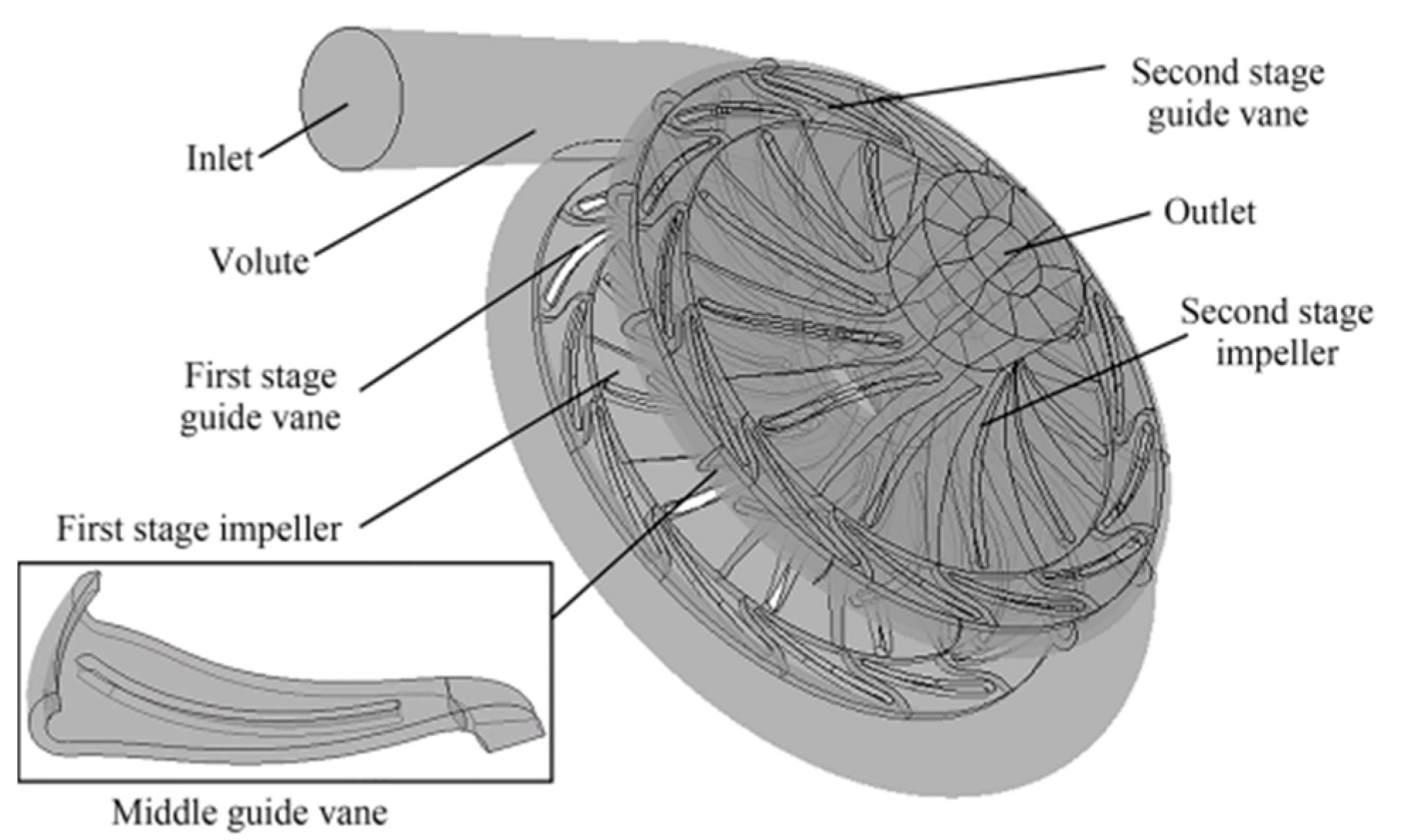
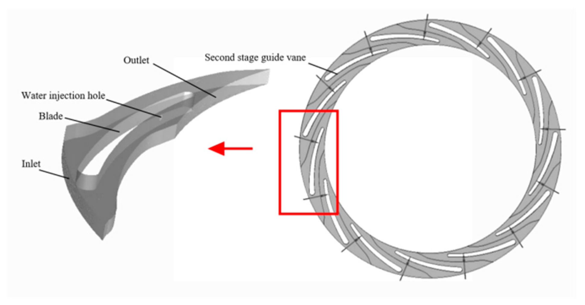
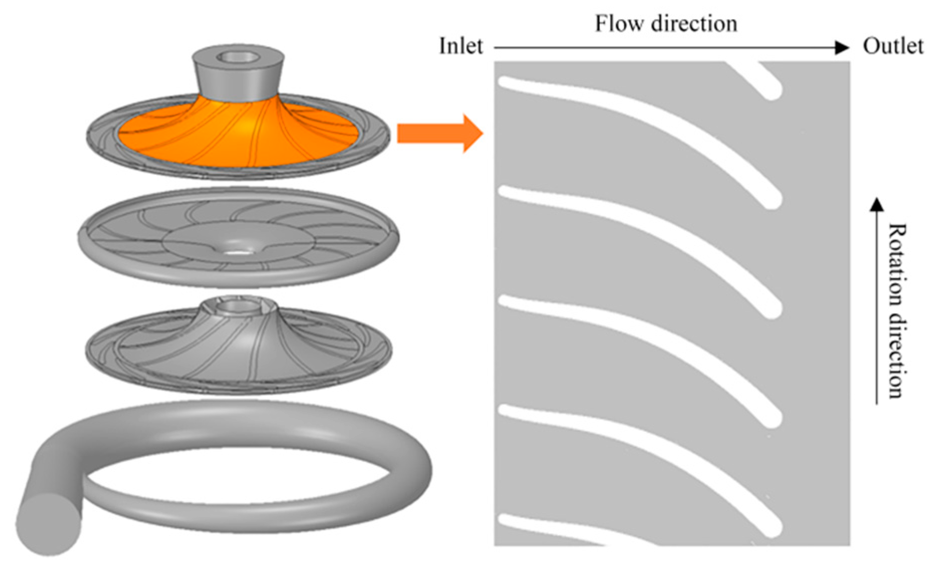
2.1. Two-Stage Hydraulic Turbine Model

The design parameters of the hydraulic turbine are listed below: design flow rate Q_d = 55.0 m³/h, rated speed n = 2985 r/min, total inlet pressure p_in = 16.5 MPa, total outlet pressure p_out = 13.5 MPa, available head H_d = 306 m under the design flow rate.

Table 1. Geometric parameters of hydraulic turbine model.

Part	Parameters	Data
Impeller	Impeller outlet diameter D1/mm	60.00
	Impeller inlet diameter D2/mm	182.00
	Impeller hub diameter Dh/mm	32.50
	Shroud blade wrap angle φf/(°)	44.50
	Hub blade wrap angle φr/(°)	36.80
	Shroud blade exit angle β1f/(°)	35.00
	Hub blade exit angle β1r/(°)	51.00
	Number of blades z	11
Volute	Base circle diameter of volute D3/mm	232.00
	Inlet tube length of volute L1/mm	120.00
	Inlet diameter of volute D4/mm	50.00

shows the geometric parameters of the hydraulic turbine, which had been designed by the self-developed design software TurboTides based on forward design method. The 3D structure is shown in Figure 1. The impellers in the model were closed impellers, and there was no clearance between the hub and shroud and the impeller blades.

Computational fluid dynamics (CFD) is widely used in the pump industry to investigate intricate flow characteristics [21,22]. In this paper, ANSYS CFX, a commercial calculation software of the finite volume method based on finite element, was used for numerical calculation, which absorbs the numerical accuracy of the finite element method on the basis of ensuring the conservation characteristics of the finite volume method. Meanwhile, the mass conservation equation, momentum conservation equation, and energy conservation equation were used as the governing equation. The detached eddy simulation (DES) method based on the SST k-ω model [23] was employed to study the two-stage hydraulic turbine. The Zwart–Gerber–Belamri model [24] was utilized as the cavitation model. The volute’s inlet boundary was designated as the flow inlet, while the average static pressure outlet was assigned as the turbine’s outlet boundary. Under the design flow conditions, the inlet flow rate was set to 15.3 kg/s, the outlet average static pressure was set to 0.3 atm. The working fluid considered was liquid water at 25 °C, with the addition of water vapor. At the inlet boundary, the volume fractions of liquid water and water vapor were set to 1 and 0, respectively. The two-stage impeller basin was set as the rotating domain, the speed was −2985 r/min, and the other basins were static domains. The dynamic and static component interfaces were configured in Transient Rotor Stator mode, while other connections were established in General Connection mode. And the steady calculation’s convergence outcome served as the initial condition for the subsequent unsteady calculation.

The convergence criteria, Root Mean Square (RMS), was set as 10⁻⁵. The computational method employed was the finite volume method. A high-resolution scheme was applied to the convective term, and the second-order backward Euler scheme was used for the transient terms. Meanwhile, an isothermal heat transfer model was used in the simulation.

The sampling interval for this simulation was 0.00008375 s, corresponding to a sampling frequency of 11,940.3 Hz. The blade passing frequency St_BPF was 547.25 Hz. According to the Nyquist sampling theorem, the sampling frequency should not exceed twice the highest frequency. The characteristic frequencies analyzed in this paper were primarily St_0.064 and St_1.182. According to Equation (4), their corresponding sampling frequencies can be calculated as 35.02 Hz and 646.85 Hz, respectively. Both frequencies fell within twice the BPF and were significantly lower than the sampling frequency of 11,940 Hz. Therefore, the time step chosen in this work meets the requirement. To reduce frequency errors, we aimed to increase the number of revolutions within the available computational resources. The total calculation time in the paper was 0.7035 s, which equaled the time of 35 revolutions of the impeller, and the frequency error was 1.4215 Hz.

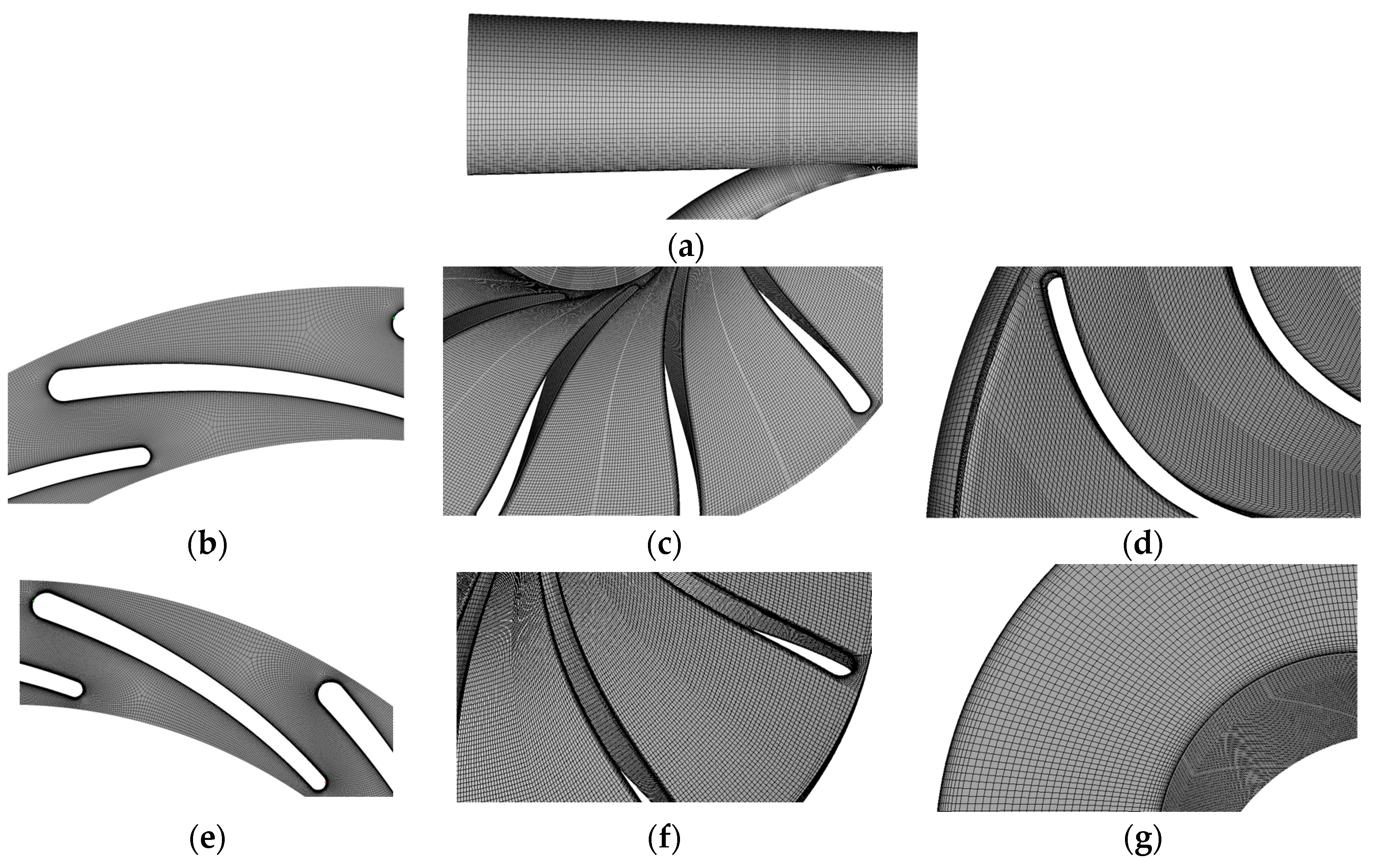
2.2. Grid Independence Analysis

In this paper, ICEM CFD was used to draw the hexahedral structured grid with better computational convergence and more efficient solution for each component of the hydraulic turbine. In order to ensure the computational efficiency and accuracy of the results, boundary layer encryption was carried out on the guide vane and impeller blades. The height, height ratio, and number of layers of the boundary layer were set to 0.001, 1.2, and 20, respectively, and the mesh quality of each component was higher than 0.3. Four distinct grid sets with varying numbers were generated, and then the mesh of each component was imported into ANSYS CFX for merging.

Details and grid independence analysis results of the 4 sets of grids are shown in

Table 2. Grid information and grid independence analysis.

Flow-Passing Parts		Grid 1	Grid 2	Grid 3	Grid 4
Volute		0.37 × 106	0.47 × 106	0.70 × 106	1.11 × 106
First-stage guide vane		0.34 × 106	0.46 × 106	0.83 × 106	1.21 × 106
First-stage impeller		1.09 × 106	1.82 × 106	2.65 × 106	3.10 × 106
Middle guide vane		0.73 × 106	1.10 × 106	1.75× 106	2.23 × 106
Second-stage guide vane		0.54 × 106	0.80 × 106	1.04 × 106	1.50 × 106
Second-stage impeller		1.34 × 106	2.09 × 106	2.90 × 106	3.31 × 106
Outlet chamber		0.32 × 106	0.64 × 106	0.93 × 106	1.38 × 106
Total grid		4.75 × 106	7.38 × 106	10.8 × 106	13.8 × 106
Result	η	75.2%	76.4%	78.9%	79.2%
	H (m)	272.57	272.50	293.92	296.37
	(H-Hd)(Hd)−1	10.9%	10.9%	3.9%	3.1%

. The difference between the computed head H and the design head H_d for Grid 3 and Grid 4, expressed as (H-H_d)/H_d, is less than 4. The calculation results tended to be stable; the calculation results for grid 3 and grid 4 differed by no more than 1%, and the efficiency of these two grids also differed by no more than 1%. Considering the computing resources and time cost, grid 3 with 10.8 million grids was selected. The details of each component of grid 3 are shown in Figure 2, in which the guide vanes and impeller blades of each stage showed that the blade surfaces of each component underwent boundary layer refinement. The maximum Y+ value on the surface of the impeller blade was less than 15, and the maximum Y+ value on the surface of the guide vanes of each stage was less than 40, and the minimum Y+ value for all the surfaces was 0.18.

3. Calculation and Analysis Methods

3.1. Cavitation Model

The DES method based on the SST k-ω model was used to develop the unsteady calculations. The Zwart–Gerber–Belamri cavitation model [25,26,27] was used for the cavitation calculations, and the mixture hybrid model was chosen for the multiphase flow model. The cavitation models [28,29] are shown in Equations (1) and (2).

When P ≤ P_vap

$$R_e=F_{vap}\frac{3{\alpha }_{nuc}(1-{\alpha }_v){\rho }_v}{R_b}\sqrt{\frac{2(p_v-p)}{3{\rho }_1}}$$

(1)

When P ≤ P_vap

$$R_c=F_{cond}\frac{3{\alpha }_v{\rho }_v}{R_b}\sqrt{\frac{2(p-p_v)}{3{\rho }_1}}$$

(2)

where R_e and R_c are the evaporation rate and condensation rate; F_vap and F_cond are the empirical coefficients of evaporation and condensation, generally taking 50 and 0.01; α_nuc is the initial volume fraction of the vacuole; α_v is the volume fraction of the vacuole; R_b is the radius of the vacuole; ρ_v and ρ₁ are the density of the vacuole, fluid work density; and p_v is the saturation vaporization pressure of the liquid work, take the saturation vaporization pressure of water at 25 degrees Celsius as 3574 Pa.

3.2. Numerical Analysis Methods

To obtain the pressure signal of the impeller flow field, the dimensionless parameter span was utilized to describe the relative surface between the hub and shroud. Three monitoring surfaces were established within the secondary impeller, as illustrated in Figure 3. Additionally, Figure 4 displayed the arrangement of flow field monitoring points within the secondary impeller, with each point positioned along the Span0.5 section of the flow channel. The monitoring points were arranged on the Span0.5 surface. The pressure strength was expressed by the dimensionless coefficient C_p [30].

$$C_p=\frac{p-\stackrel{\_}{p}}{\rho u^2/2}\times 100\%$$

(3)

where p is the instantaneous pressure value of the monitoring point, $\stackrel{\_}{p}$ is the local average pressure, u is the circumferential velocity of the outer diameter of the impeller, and ρ is the density of water.

We employed the Strouhal number (St) [31] to non-dimensionalize the frequency of pressure pulsations:

$$St=\frac{f}{f_{BPF}}$$

(4)

where f is the frequency and f_BPF is the blade passing frequency. For the turbine rotor blades studied in this paper, the passing frequency f_BPF is 547.25 Hz. Utilizing Equation (4), the corresponding Strouhal number St_BPF is calculated as 1, indicating St = 1.

POD is a widely used method of processing large amounts of data in image processing and signal analysis, among others [32]. The flow field snapshot POD method was used in this study since the spatial dimension was higher than the temporal one, which considered a collection of flow field observations at a series of discrete moments [33]. The eigenvalues of each POD mode reflected the energy contribution of this mode to the flow field so as to obtain the main high-energy POD mode of the flow field. Based on arranging the spatial coordinates of grid nodes, the spatial distribution of the flow field of each mode could be obtained by combining it with the POD mode [34].

Using pressure as the characteristic quantity of the flow field, the pressure data of each grid node at a certain discrete moment could be arranged in a column vector p(x, t_i) in a specific spatial order, which served as a snapshot of the flow field. The collection of flow field snapshots could be represented as follows:

$$U^n={\{p(x,t_i)\}}_{i=1}^n$$

(5)

where p represents the pressure value of the flow field; x represents the sequence number of each grid node; t_i represents the discrete moments; and n represents the number of flow field snapshots. Among them, the characteristic quantities of the flow field at each moment can be seen as the superposition of the fundamental flow and fluctuating pressure values:

$$p(x,t_i)=p_0(x,t_i)+p^{\prime }(x,t_i)$$

(6)

By employing the POD method, the fluctuating component could be orthogonally decomposed. It could be expressed using the product of the POD modal coefficient a_j and the modal basis Φ_j:

$$p^{\prime }(x,t_i)={\displaystyle \sum _{j=1}^n{a}_j(t_i)}{\Phi }_j(x)$$

(7)

where Φ_j(x) represents the POD modal basis, and a_j(t_i) represents the modal coefficient of the jth POD basis at time t_i.

To obtain the POD modal basis, the relevant matrix C was computed:

$$C=P^{T}P$$

(8)

$$P=\left[p^{\prime }(x,t_1)p^{\prime }(x,t_2)\cdots p^{\prime }(x,t_n)\right]$$

(9)

$$C{A}_j={\lambda }_j{A}_j$$

(10)

where P represents a sequence matrix composed of n discrete moment flow field snapshot pressure fluctuation data. C denotes the correlation matrix, which is a symmetric matrix. j represents the jth eigenvalue of the POD mode, while A_j represents the corresponding eigenvector.

The formulas for the modal coefficient a_j and modal basis Φ_j of each POD mode are as follows:

$$a_j={\Phi }_j{}^{T}P$$

(11)

$${\Phi }_j=P{A}_j/\sqrt{{\lambda }_j}$$

(12)

The magnitudes of the eigenvalues of each POD mode reflected the contribution of that mode to the energy of the flow field. By sorting the POD modes according to their energy contribution, we could further identify the main high-energy POD modes of the flow field. Additionally, by performing a Fourier transform on the modal coefficients a_j corresponding to the high-energy modes, we could extract the characteristic frequencies associated with those modes.

To obtain the distribution characteristics of unsteady flow structure and pulsation in a two-dimensional space, the frequency domain visualization analysis method of a two-dimensional flow field characteristic quantity of unsteady flow proposed by Yang et al. [35] was used.

The time domain signal distribution of the flow field in the whole monitoring surface in unsteady flow was obtained by numerical simulation. These time domain signals of the one-dimensional characteristic quantities were processed by Fast Fourier Transform (FFT) to obtain their discrete peak frequency and corresponding amplitude magnitudes. Then, the high-order spectrum analysis of these one-dimensional characteristic signals in the time domain was performed to obtain their nonlinear frequencies in the frequency domain.

Combined with the nonlinear frequency of each monitoring surface, the two-dimensional frequency domain distribution database of the flow field characteristics corresponding to the flow field monitoring surface was obtained by the time-frequency domain conversion method. The characteristic frequency of the unsteady flow structure in this region was determined by comparing the high amplitude region in the database with the unsteady flow region, and then the two-dimensional distribution figure of the flow field characteristic quantity corresponding to the characteristic frequency was extracted from the database. The figure could show the distribution of flow field characteristics in each flow component at this characteristic frequency and could visually observe the distribution position, shape, and strength of the unsteady flow structure.

3.3. Compressible Model

Given the relatively negligible temperature variations during the working conditions, a constant temperature assumption was made for the simulation. Yang et al. [36] simplified the original function representing the density of water in terms of temperature and pressure using the Tait equation, resulting in a revised function solely dependent on pressure:

$$\rho ={\rho }_0+{\left(1+\frac{n\left(p-p_0\right)}{k_0}\right)}^{\frac{1}{n}}$$

(13)

where p₀ is the reference pressure of water at 25 °C, ρ₀ is the density of water under the reference pressure p₀, k₀ is the reference pressure of the bulk modulus (2.2103 MPa), n is the density index and taken 7.15, p is the pressure of water, and ρ is the density of water under the pressure p. The pressure in the formula is absolute pressure.

The present study employed ANSYS CFX 2019 software to implement Equation (13) through the CFX Command Language (CCL) to consider the weak compressibility of water in the numerical calculations. The outcomes revealed that when the number of grids and CPU were the same, the compressibility increased the calculation time, but the overall calculation was friendly. Therefore, it was suitable for this simulation.

In this simulation, this compressible model based on the Tait–Murnaghan equation worked only in the liquid phase. When the pressure of the flow field was less than the saturation vaporization pressure (3574 Pa in this simulation setting), the working medium changed from the liquid phase to the vapor phase. At this time, the model did not work, and the cavitation model (Zwart–Gerber–Belamri model) worked.

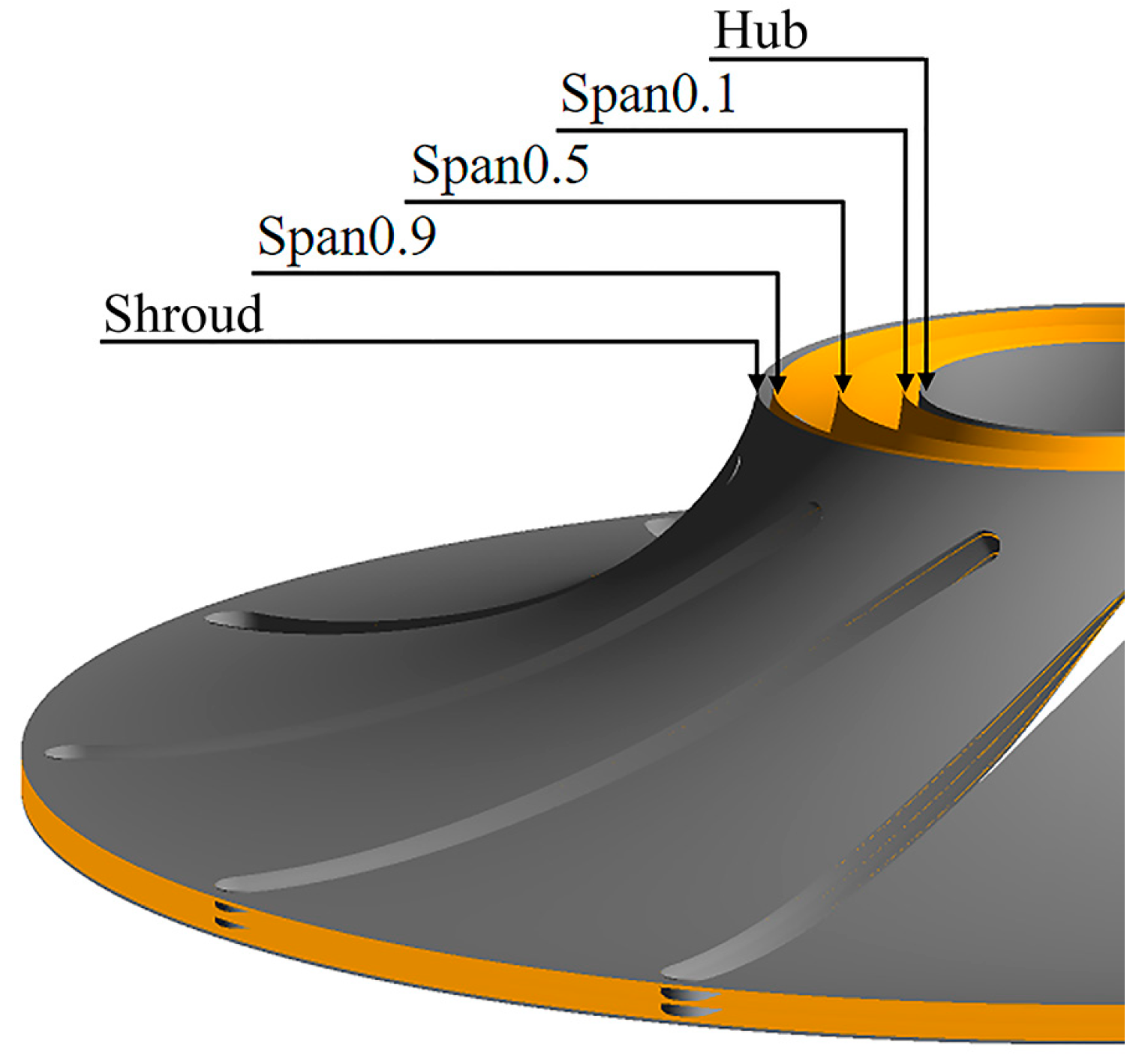
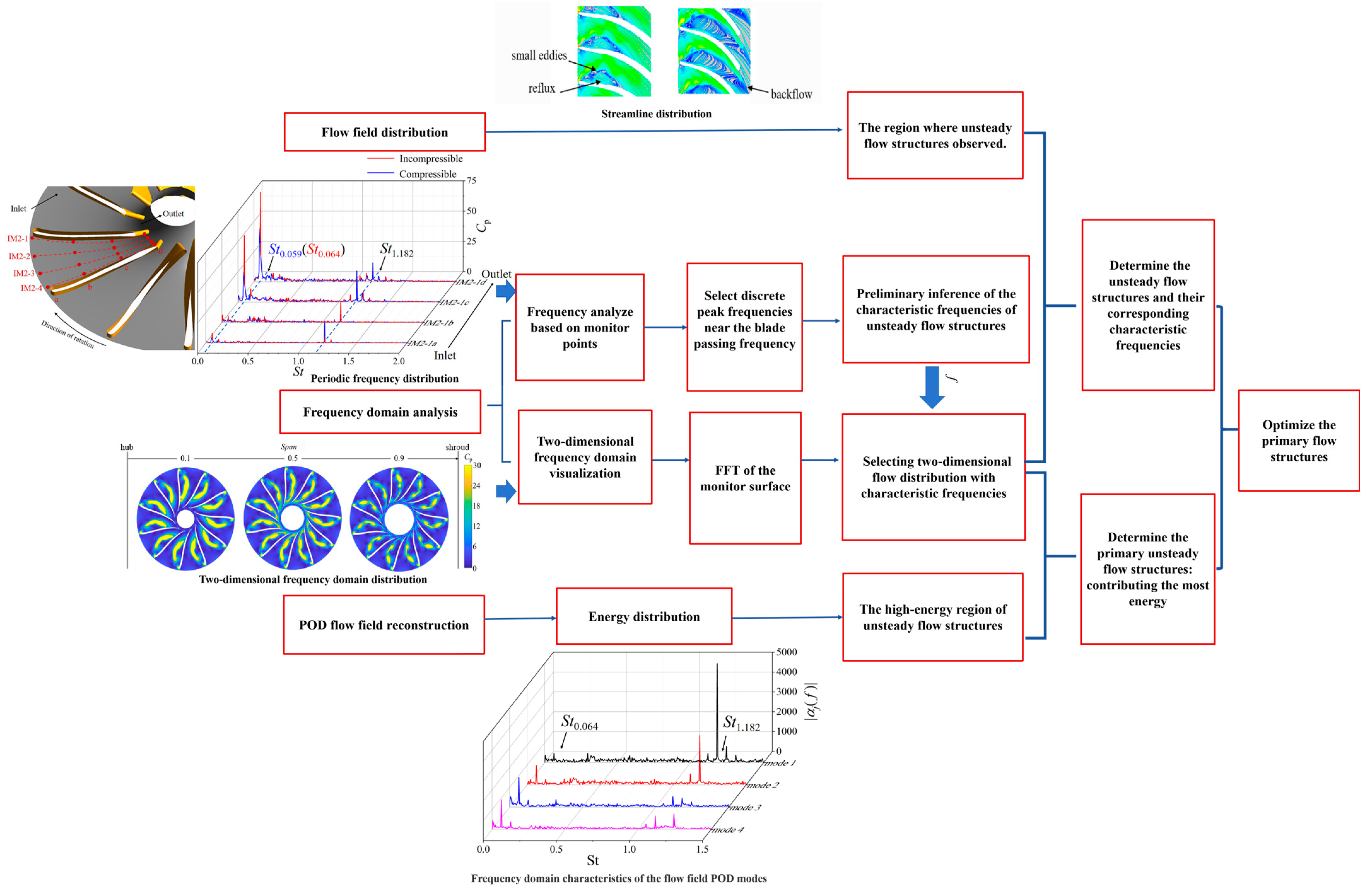
3.4. Flow Field Analysis Methods

The present study introduces a novel approach to analyze and optimize the unsteady flow within a turbine impeller, as shown in Figure 5. Firstly, intuitive spatial flow distribution can be obtained through the flow field distribution in the impeller, such as streamline, velocity contour, vorticity, etc. As certain unsteady flows may become intricate, arising from the superposition of several interacting flow structures, it is often challenging to discern their specific characteristics directly from the flow distribution.

Consequently, frequency domain analysis is employed to identify the influence of pulsations at periodic frequencies within the flow field. This study primarily focuses on analyzing discrete peak frequency pulsations near the blade passing frequency (BPF) and below the BPF. Some of these frequency peaks correspond to the harmonic frequency of some unsteady flow structures, while others may be the linear superposition of several unsteady flow characteristic frequencies.

Through the traditional frequency analysis, discrete and prominent frequency peaks in the flow filed (such as pressure, velocity, etc.) are observed. The next step is to find the characteristic frequencies of the periodic unsteady flows that caused these discrete frequencies.

Subsequently, a two-dimensional frequency domain visualization method is employed to display the intensity of flow distribution at these characteristic frequencies. This process aims to obtain a two-dimensional flow distribution at frequencies corresponding to the flow structure on the monitoring surface.

Taking pressure pulsation as an example, the detailed implementation is as follows. Fast Fourier transform (FFT) was carried out on the pressure of monitoring points on the whole monitoring surface to obtain the pressure pulsation intensity distribution at different frequencies. These flow distribution diagrams are then compared with the unsteady flow in the first-step intuitive spatial flow distribution to identify the shape and flow characteristics of the corresponding flow structure.

At the same time, there are many unsteady flow structures in complex flow fields. Determining which is the main factor causing the problem under this working condition is also the focus and difficulty of our optimization design. To solve this problem, the Proper Orthogonal Decomposition (POD) method is adopted to ascertain the specific energy contribution of the flow structures to the flow field. The flow field data are reconstructed by using the Proper Orthogonal Decomposition (POD) method, yielding the energy distribution of the flow field and the high-energy regions of the flow structures.

Subsequently, through further comparison with the two-dimensional frequency domain distribution map, the primary flow structures within the unsteady flow regime, those exerting the greatest influence on the flow field and contributing the most energy, are elucidated. When optimizing the flow field, priority can be given to the optimization of these primary flow structures.

4. Effect of Working Fluid Compressibility in the Last-Stage Impeller

During the calculation, it was observed that the presence of liquid vaporization was noticeable within the turbine with the decrease in outlet pressure. The distribution of cavitation within the turbine at the designed flow rate is illustrated in Figure 6. The accumulation of cavitation was predominantly located in the channel of the secondary impeller and the proximity to the impeller outlet as the outlet static pressure decreased to 0.3 atm.

Therefore, when the outlet pressure decreased, the area where two-phase flow was most likely to occur was the impeller of the second stage, and the cavitation zone of the impeller is analyzed below. To enable an intuitive description and analysis of the flow field of the impeller, the radial cross sections of different span values of the secondary impeller were established, and the structure is shown in Figure 7.

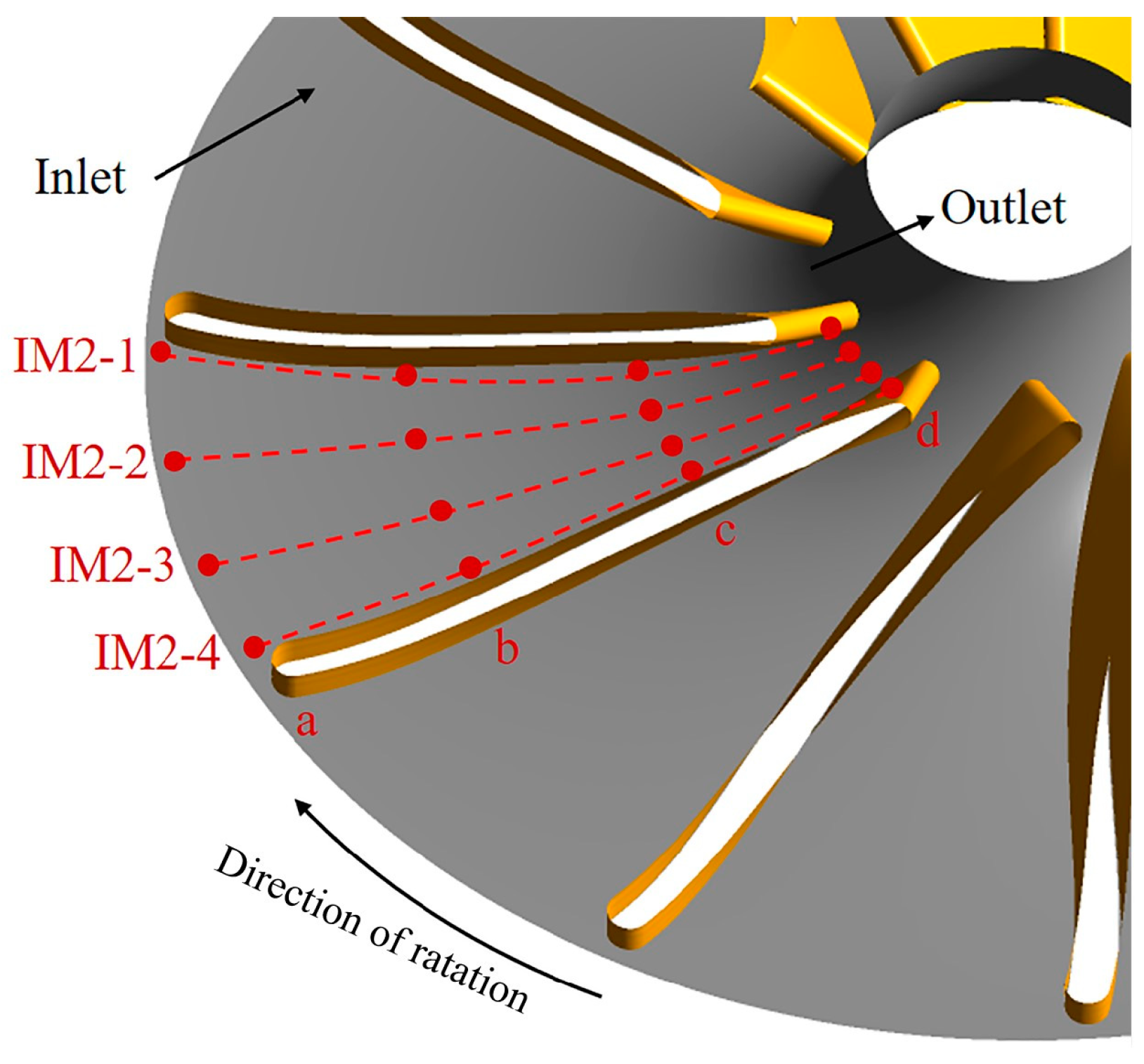
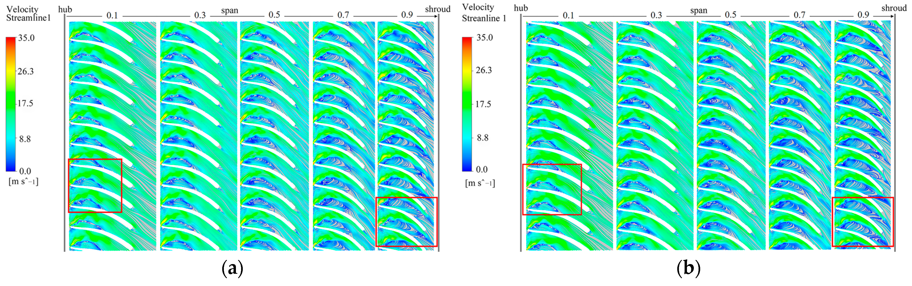
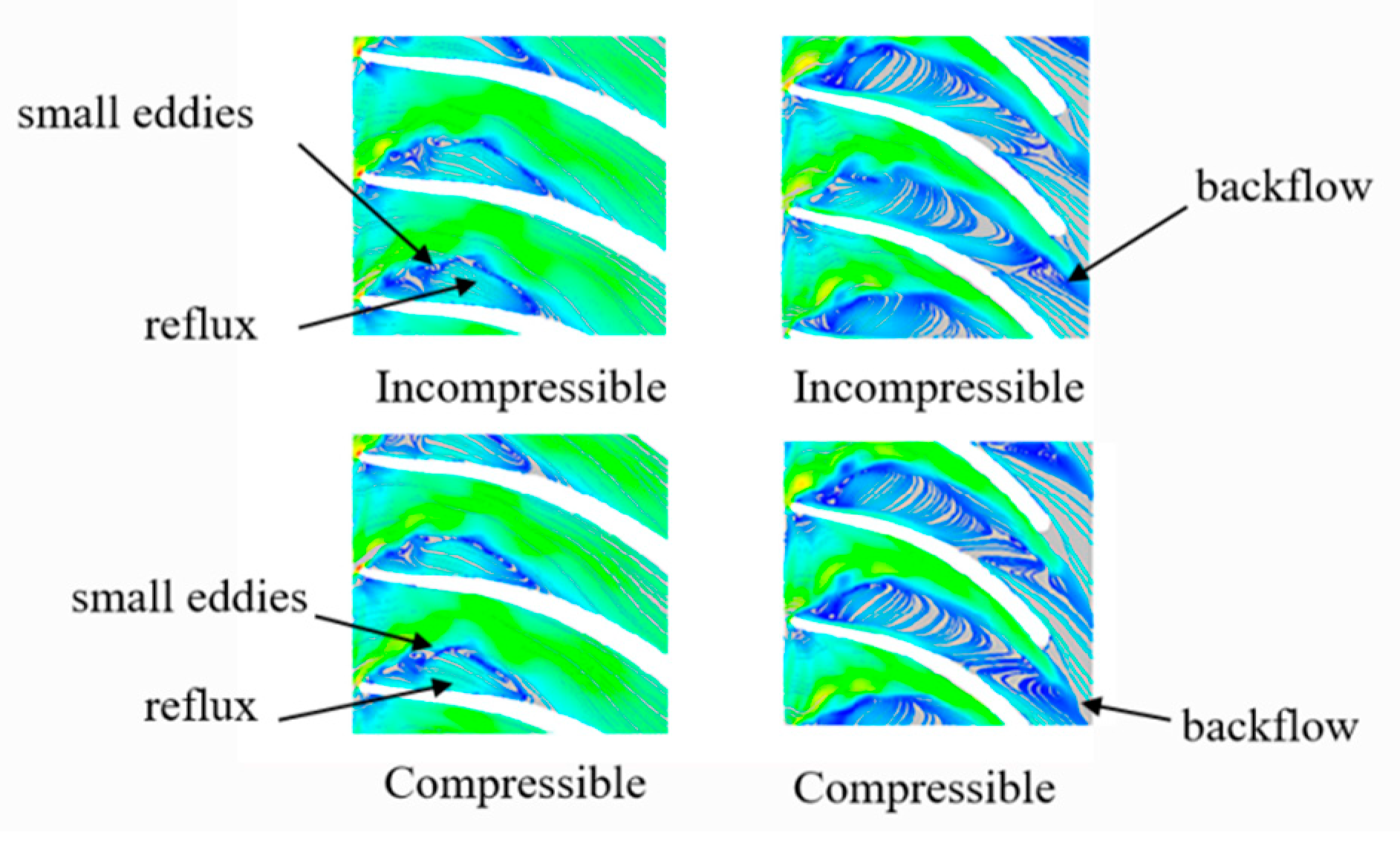
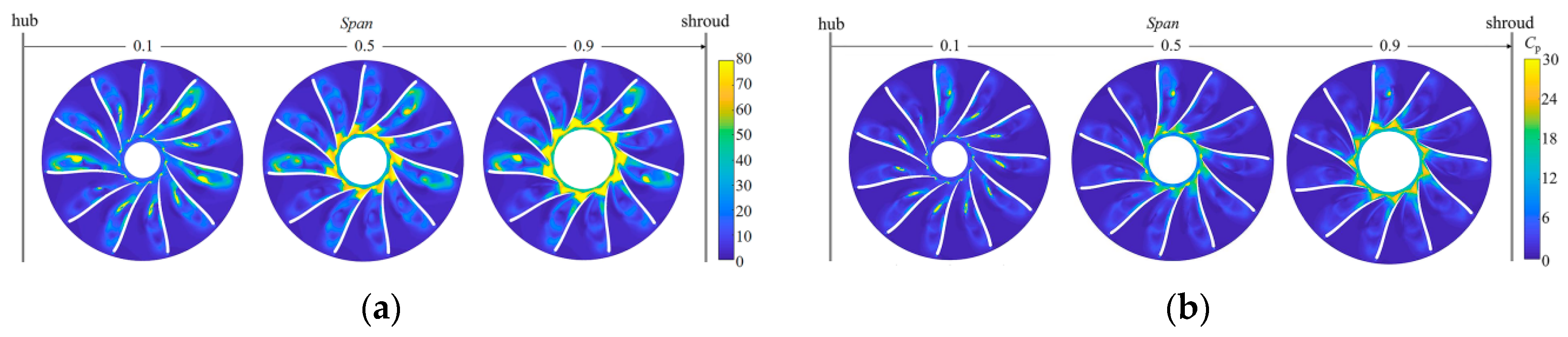
4.1. Flow Field Analysis of the Last-Stage Impeller

The comparison of the flow field in the last-stage impeller with and without considering the compressibility of the liquid phase is illustrated in Figure 8, and the details can be seen in Figure 9. It can be observed from Figure 8 that irrespective of whether compressibility was considered or not, two distinct flow structures manifested within the impeller runner. Firstly, a significant reflux region was evident near the suction surface of the impeller inlet, with its size correlating to that of the cavitation area. Additionally, several small eddies were observed along the outer edge of this reflux, near the leading edge of the blade, and gradually increased in magnitude towards the shroud direction.

Another noteworthy flow structure was identified as the backflow occurring in the vicinity of the outlet and shroud regions. In this region, the influence of compressibility on the liquid phase was prominently pronounced.

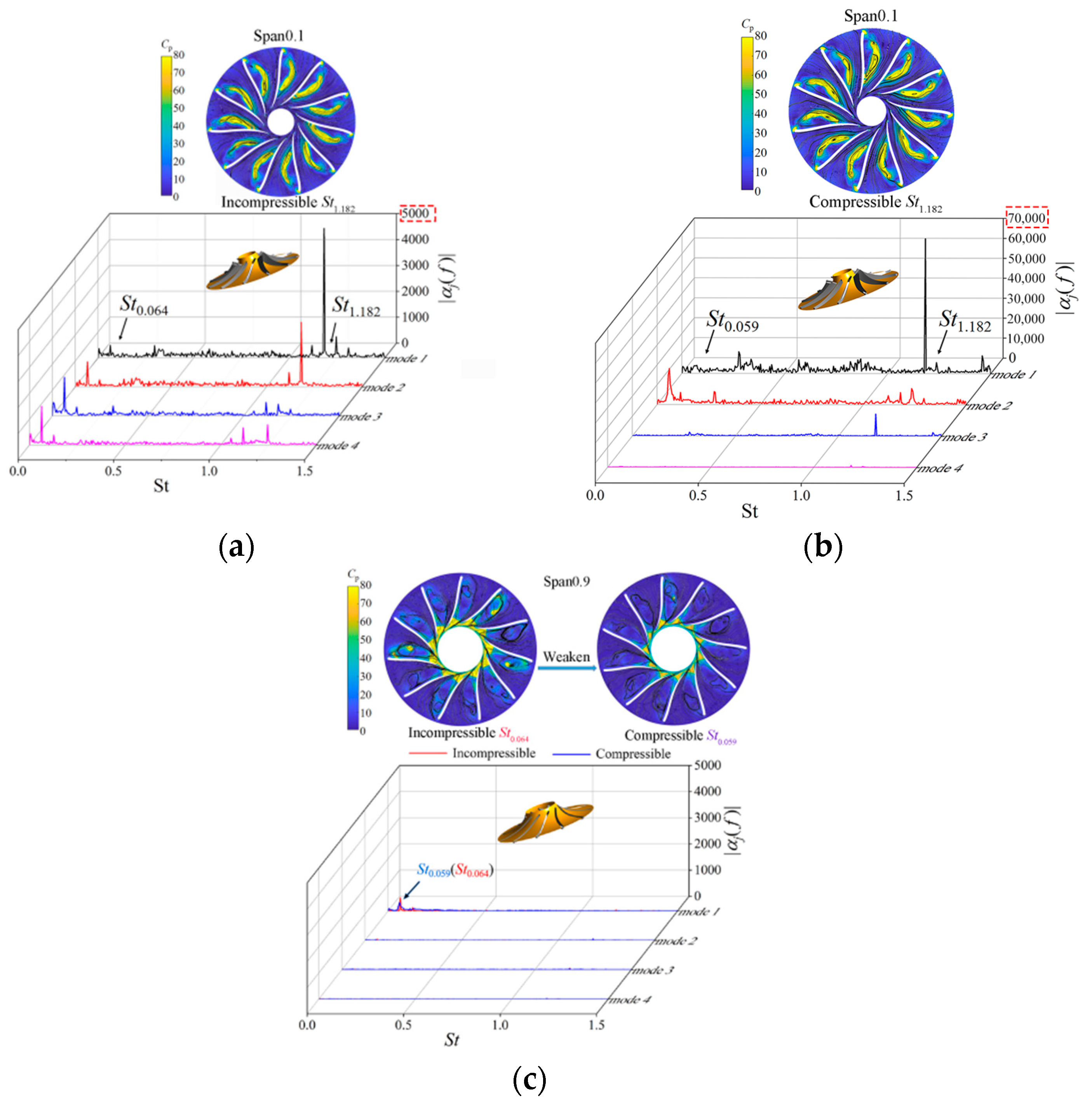
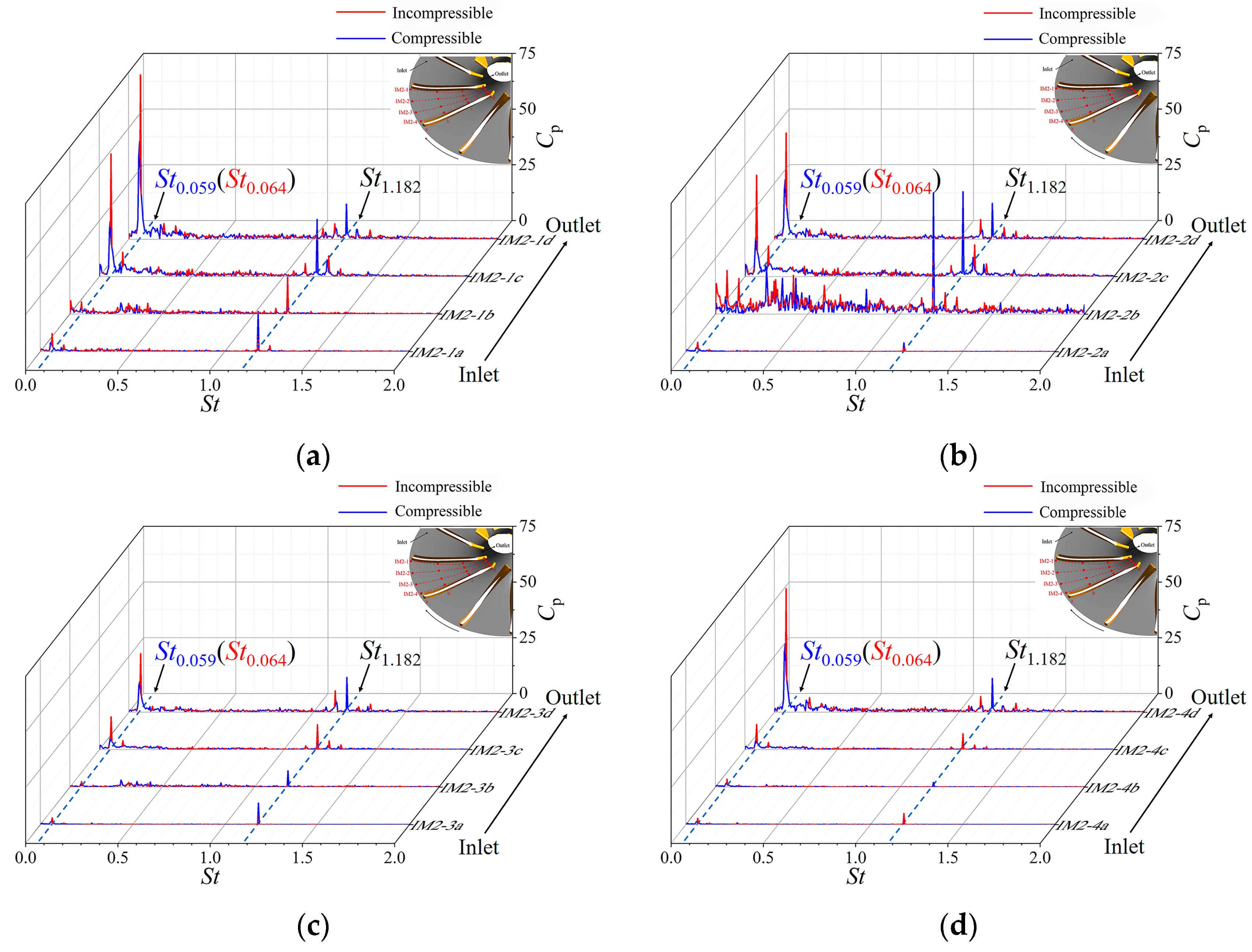
4.2. Pressure Spectrum Analysis of Secondary Impeller

To conduct a more comprehensive examination of these two flow structures within the impeller, an analysis of pressure pulsation was conducted. Spectrum analysis of pressure pulsation at each monitoring point within the secondary impeller was undertaken to identify the primary contributions of pressure pulsation occurring inside the impeller. As depicted in Figure 10, in the absence of considering the compressibility of water, the prominent frequency peaks were mainly observed at St_0.064 and St_1.182. St_1.182 is identified as a linear superposition frequency of the blade passing frequency St = 1 (St_BPF) and the characteristic frequency St_0.064, expressed as St_1.182 ≈ St_BPF + 3 St_0.064. In Figure 10b, the monitoring points are located near the middle of the flow channel, and all kinds of unsteady flows develop completely. Therefore, in addition to the peaks detected in other detection lines (St_0.064 and St_1.182), there are many small pulsating peaks below the frequency of the blade passing frequency St_BPF.

Upon considering the compressibility, the frequency peak below the BPF shifted to St_0.059, with a frequency sampling error of ΔSt = 0.0045; it could be presumed that the discrete frequencies St_0.064 and St_0.059 were caused by the same unsteady flow structure. Regarding the amplitude at this frequency, the results indicated that the pulsation was more pronounced when the water compressibility was not considered. The peak value of the pressure fluctuation amplitude C_p for characteristic frequency St_0.064 occurred at IM2-1d (impeller outlet), and considering compressibility, the peak value decreased from 72 to 59. For characteristic frequency St_1.182, the peak value of C_p occurred at IM2-2b (within the impeller passage), and considering compressibility, the peak value slightly increased from 50 to 52.

Consequently, a preliminary deduction could be made that the secondary impeller encompassed two primary unstable flow structures: one was around St_0.064 and the other was St_1.182. Additionally, it was noteworthy that the compressibility of the water exhibited distinct implications on these two structures.

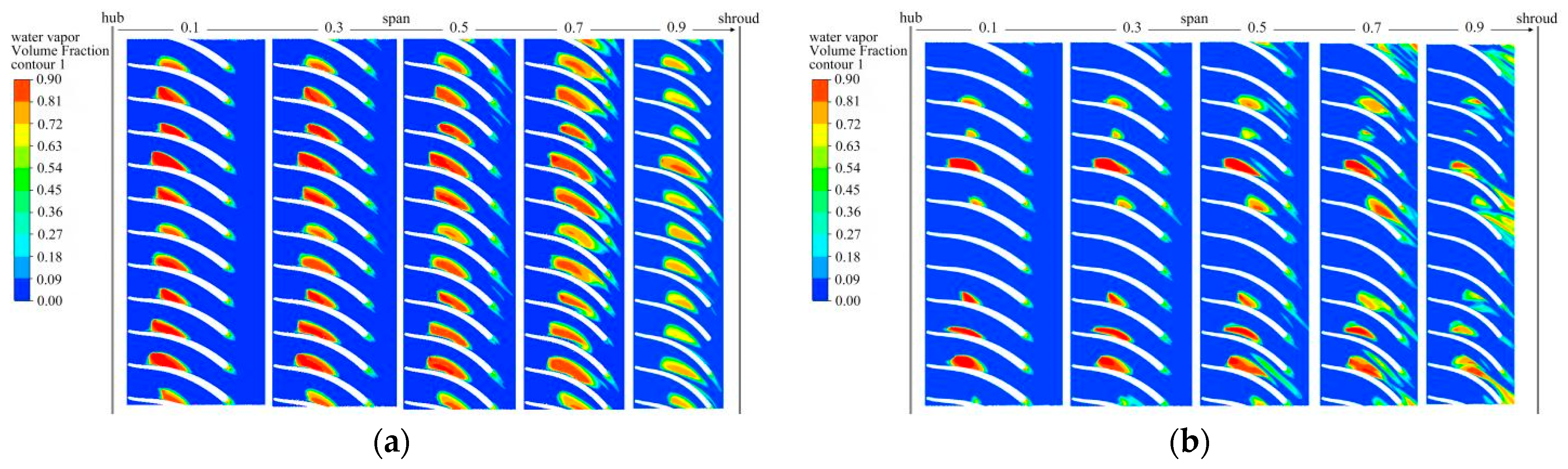
4.3. Analysis of the Distribution of Unsteady Flow Structures in the Secondary Impeller

This section primarily focuses on the spatial distribution analysis of the flow structure corresponding to the two characteristic frequencies within the impeller, illustrated in Figure 11 and Figure 12.

Figure 11 presents the two-dimensional distribution of the pressure pulsation amplitude for both incompressible and compressible results at the characteristic frequency St_0.064 within the secondary impeller. It is evident that the region with high amplitude is predominantly concentrated at the outlet of the impeller, with the most pronounced occurrence observed near the shroud (Span0.9). This feature was consistent with the previous analysis of the outlet backflow characteristics. Therefore, it was inferred that the characteristic frequency of the outlet backflow was St_0.064. Furthermore, the comparison results showed that considering the compressibility of the fluid, the peak value of the pressure fluctuation amplitude C_p decreased significantly by 18.1%, and the strength and area of the backflow were both reduced in the calculation results.

For the characteristic frequency St_1.182, as depicted in Figure 12, the high amplitude region of this frequency was predominantly located on the suction surface of the impeller, with the most pronounced occurrence observed near the hub (Span0.1). This observation aligned with the presence of the reflux and the small eddies along the outer edge of this reflux. Furthermore, the pressure amplitude analysis revealed that the pressure fluctuation intensity of these small eddies surpassed that of the inner reflux, with the intensity gradually diminishing from the hub towards the shroud. And, considering the compressibility, the action strength of the small eddies was slightly increased, and the peak value of the pressure fluctuation amplitude C_p increased by 4%.

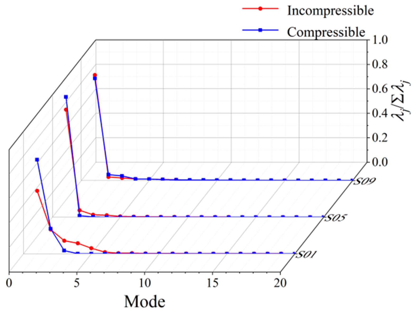
4.4. Analysis of Energy Distribution of Flow Field Based on POD

In this section, we aim to analyze the energy distribution of the unsteady flow structures of the flow field in the second impeller.

Based on the aforementioned analysis, two prominent flow structures with characteristic frequencies were identified within the secondary impeller: St_0.064, associated with the backflow at the impeller outlet and predominantly occurring near the shroud; and St_1.182, corresponding to a significant flow structure on the suction side of the impeller. The subsequent section aims to analyze the energy ratio of these two flow structures, employing the POD method.

In Figure 13, the energy distribution of the pressure pulsation was presented as follows. The first 20 orders at each monitoring surface of the impeller, both with and without considering the compressibility of water, were ranked, and the comparison revealed that the first-order mode had the largest proportion of energy at each monitoring surface. Notably, at Span0.1 and Span0.5, the peak value of the first order mode increased by 49.3% and 10.2%, respectively, while at Span0.9, it decreased by 3.2%. In the subsequent analysis, we selected the first four orders for frequency domain analysis.

In Figure 14, a comparison of the first four POD modes was conducted in the frequency domain for each monitoring surface of the impeller. The analysis revealed that the periodic flow structure exhibiting the characteristic frequency St_1.182 near the hub played a significant role as the primary contributor to the pulsation energy within the flow field. Additionally, it was observed that the flow structure corresponding to St_1.182 not only served as the most dominant energy contributor at the hub but was also notably influenced by the compressibility of water. As shown in Figure 14a,b, for Span0.1, the peak value of the modal coefficient of St_1.182 increased from 5560 to 67,710, which increased by nearly 1120%, and the pressure pulsation amplitude also increased. This indicates that the energy proportion of the flow structure near the hub corresponding to St_1.182 in the flow channel was significantly amplified, and its reflux degree was more serious.

In contrast, in Figure 14c, for the periodic pulsation with the characteristic frequency St_0.064, the modal coefficient at Span0.9 decreased by 32.2%. At the same time, the two-dimensional amplitude of the pressure pulsation was also reduced. That means the strength and area of the backflow near the shroud corresponding to St_0.064 were both reduced.

5. Optimization Scheme

In this section, we address the schema optimization aimed at enhancing the two-phase flow issues within the secondary impeller.

Based on the analysis conducted in the preceding section, the flow structure exhibiting the maximum energy ratio relative to the two-phase flow zone of the secondary impeller was identified as the small eddies encircling the reflux, characterized by the frequency St_1.182, near the inlet leading edge of the suction surface of the impeller. Consequently, we devised a strategy to mitigate the backflow arising from flow separation at the inlet leading edge of the secondary impeller by modifying the upstream flow field. Specifically, we introduced a controlled water injection, with a predetermined velocity, through the opening hole of the second-stage guide vane. The schematic diagram of this approach is depicted in Figure 15.

At the trailing edge of the second-stage fixed guide vane, a hole was opened near the trailing edge of each vane in the middle between hub and shroud to inject water. The aperture of the water injection hole was 1.4 mm. The velocity coefficient C_v calculated by Equation (14) was used for dimensionless processing of transient velocity fluctuations.

$$C_v=\frac{v-\overline{v}}{\overline{v}}$$

(14)

where v represents the instantaneous velocity value of the monitoring point, and $\stackrel{\_}{v}$ is the average velocity of for a while.

The direction of water injection in the hole is shown by the black arrow in Figure 15. The speed C_v = 0.173 was slightly greater than the flow speed of water in the second-stage guide vane.

The internal flow field of the two-stage impeller after water injection is shown in Figure 16 and Figure 17. Figure 16b illustrates the vapor distribution of the two-stage impeller following the optimization of water injection. It is evident that significant improvements have been achieved. Compared to the previous state, the vapor volume in some portions of the flow passage has decreased to 0, and in other sections of the flow passage has also decreased by 30% to 40%. According to the flow field distribution in Figure 17b, the small eddies with a characteristic frequency of St_1.182 were well suppressed.

Figure 18 presents the two-dimensional amplitude distribution of pressure pulsations corresponding to characteristic frequency St_1.182 before and after optimization. The spatial distribution of the characteristic frequency St_1.182 is notably attenuated, providing evidence that the water injection optimization strategy effectively enhances the unsteady flow structures.

6. Conclusions

For this small-scale hydraulic turbine, the last stage impeller is the area with the lowest pressure and the most complex flow structure, with a high risk of vaporization. Meanwhile, the results of considering the compressibility of the working medium could capture more details regarding the flow structures. And the proposed optimization scheme could effectively improve the unsteady flow structures in the flow field. The specific conclusions are as follows:

• Based on the analysis of POD and two-dimensional frequency domain visualization and flow field distribution, it was found that the last stage impeller has two main flow structures, which were the areas with high risks of vaporization under this study condition. The corresponding characteristic frequencies were St_0.064 and St_1.182.
• The flow structure of St_1.182 also had a high risk of forming an evaporation zone on the suction surface of the impeller near the hub. This flow structure was composed of a large reflux and some small eddies at the outer edge of the reflux. These small eddies were near the leading edge of the suction side of impeller blades and they were the largest energy contributor in the impeller. The impact of water compressibility on the internal flow structures was a significant factor that should not be ignored. The flow structures of St_1.182 demonstrate amplified pressure fluctuations, while the other one exhibited reduced pressure fluctuations.
• The strategy of water injection in the upstream guide vane could mitigate the backflow arising from flow separation at the inlet leading edge of the secondary impeller to alleviate the vapor–liquid two-phase flow in this area. That means the analysis of space, frequency, and energy distribution had a good effect on the evaluation of unsteady flow structures in the flow field, which provided a direction for the establishment of the diagnosis and optimization framework of unsteady flow structures in rotating machinery.

References

1. Zhang, Y.; Luo, H.; Wang, C. Progress and trends of global carbon neutrality pledges. Adv. Clim. Chang. Res. 2021, 17, 88–97. [Google Scholar]
2. Peng, C.D. Contribute to the realization of the goal of “carbon peak and carbon neutrality” speed up the development of pumped storage power plants. Hydropower Pumped Storage 2021, 7, 4–6. [Google Scholar]
3. Liu, X.; Pang, J.; Li, L.; Zhao, W.; Wang, Y.; Yan, D.; Zhou, L.; Wang, Z. Comparative Study on Numerical Calculation of Modal Characteristics of Pump-Turbine Shaft System. J. Mar. Sci. Eng. 2023, 11, 2068. [Google Scholar] [CrossRef]
4. Nautiyal, H.; Varun; Kumar, A. Reverse running pumps analytical, experimental and computational study: A review. Renew. Sustain. Energy Rev. 2010, 14, 2059–2067. [Google Scholar] [CrossRef]
5. Yang, J.; Zhang, X.; Wang, X.; Sun, Q.; Zhang, J. Overview of research on energy recovery hydraulic turbine. Fluid Mach. 2011, 39, 29–33. [Google Scholar]
6. Varaksin, A.Y.; Ryzhkov, S.V. Vortex Flows with Particles and Droplets (A Review). Symmetry 2022, 14, 2016. [Google Scholar] [CrossRef]
7. Wang, Y.; Li, M.; Liu, H.L.; Chen, J.; Lv, L.L.; Wang, X.L.; Zhang, G.X. Optimized Geometric Structure of a Rotational Hydrodynamic Cavitation Reactor. J. Appl. Fluid Mech. 2023, 16, 1218–1231. [Google Scholar]
8. Yang, J.; Zhou, L.; Wang, Z. The numerical simulation of draft tube cavitation in Francis turbine at off-design conditions. Eng. Comput. 2016, 33, 139–155. [Google Scholar] [CrossRef]
9. Escaler, X.; Ekanger, J.V.; Francke, H.H.; Kjeldsen, M.; Nielsen, T.K. Detection of Draft Tube Surge and Erosive Blade Cavitation in a Full-Scale Francis Turbine. J. Fluids Eng. 2015, 137, 1676–1685. [Google Scholar] [CrossRef]
10. Liu, J.; Liu, S.; Wu, Y.; Jiao, L.; Wang, L.; Sun, Y. Numerical investigation of the hump characteristic of a pump–turbine based on an improved cavitation model. Comput. Fluids 2012, 68, 105–111. [Google Scholar] [CrossRef]
11. Minakov, A.V.; Platonov, D.V.; Dekterev, A.A.; Sentyabov, A.V.; Zakharov, A.V. The analysis of unsteady flow structure and low frequency pressure pulsations in the high-head francis turbines. Int. J. Heat Fluid Flow 2015, 53, 183–194. [Google Scholar] [CrossRef]
12. Xiao, Y.X.; Wang, Z.W.; Yan, Z.G.; Li, M.A.; Xiao, M.; Liu, D.Y. Numerical analysis of unsteady flow under high-head operating conditions in francis turbine. Eng. Comput. 2010, 27, 365–386. [Google Scholar]
13. Liu, R.S.; Zhang, L.; Li, Y.M.; Wang, K. Analysis of Internal Flow Characteristics of Fuel Centrifugal Pump. Constr. Mach. Equip. 2023, 54, 88–96. [Google Scholar]
14. Jafarzadeh Juposhti, H.; Maddahian, R.; Cervantes, M.J. Optimization of axial water injection to mitigate the Rotating Vortex Rope in a Francis turbine. Renew. Energy 2021, 175, 214–231. [Google Scholar] [CrossRef]
15. Resiga, R.; Vu, T.; Muntean, S.; Ciocan, G.; Nennemann, B. Jet Control of the Draft Tube Vortex Rope in Francis Turbines at Partial Discharge. In Proceedings of the 23rd IAHR Symposium Conference, Gdansk, Poland, 12–14 September 2022; pp. 67–80. [Google Scholar]
16. Muntean, S.; Resiga, R.; Bosioc, A. 3D Numerical Analysis of Unsteady Pressure Fluctuations in a Swirling Flow without and with Axial Water Jet Control. In Proceedings of the 14th International Conference on Fluid Flow Technologies (CMFF’09), Budapest, Hungary, 9–12 September 2009; Volume 2, pp. 510–518. [Google Scholar]
17. Deniz, S.; von Burg, M.; Tiefenthaler, M. Investigation of the Flow Instabilities of a Low Specific Speed Pump Turbine Part 2: Flow Control with Fluid Injection. J. Fluids Eng. 2022, 144, 071210. [Google Scholar] [CrossRef]
18. Deniz, S.; Del Rio, A.; von Burg, M.; Tiefenthaler, M. Investigation of the Flow Instabilities of a Low Specific Speed Pump Turbine Part 1: Experimental and Numerical Analysis. J. Fluids Eng. 2022, 144, 071209. [Google Scholar] [CrossRef]
19. Lewis, B. Improving Unsteady Hydroturbine Performance during Off-Design Operation by Injecting Water from the Trailing Edge of the Wicket Gates; The Pennsylvania State University: State College, PA, USA, 2014. [Google Scholar]
20. Khullar, S.; Singh, K.M.; Cervantes, M.J.; Gandhi, B.K. Numerical Analysis of Water Jet Injection in the Draft Tube of a Francis Turbine at Part Load Operations. J. Fluids Eng. 2022, 144, 111201. [Google Scholar] [CrossRef]
21. Osman, F.K.; Zhang, J.; Lai, L.; Kwarteng, A.A. Effects of Turbulence Models on Flow Characteristics of a Vertical Fire Pump. J. Appl. Fluid Mech. 2022, 15, 1661–1674. [Google Scholar]
22. Chen, J.; Zheng, Y.; Zhang, L.; Chen, X.; Liu, D.; Xiao, Z. Influence Analysis of Runner Inlet Diameter of Hydraulic Turbine in Turbine Mode with Ultra-Low Specific Speed. Energies 2023, 16, 7086. [Google Scholar] [CrossRef]
23. Lai, H.; Wang, H.; Zhou, Z.; Zhu, R.; Long, Y. Research on Cavitation Performance of Bidirectional Integrated Pump Gate. Energies 2023, 16, 6784. [Google Scholar] [CrossRef]
24. Song, Y.; Fan, H.; Huang, Z. Study on radial force characteristics of double-suction centrifugal pumps with different impeller arrangements under cavitation condition. Proc. Inst. Mech. Eng. Part A J. Power Energy 2021, 235, 421–431. [Google Scholar] [CrossRef]
25. Fu, Y.; Xie, J.; Shen, Y.; Pace, G.; Valentini, D.; Pasini, A.; D’Agostino, L. Experimental and numerical study on cavitation performances of a turbopump with and without an inducer. Proc. Inst. Mech. Eng. Part G J. Aerosp. Eng. 2022, 236, 1098–1111. [Google Scholar] [CrossRef]
26. Yuan, J.; Hou, J.; Fu, Y.; Hu, J.; Zhang, H.; Shen, C. A study on the unsteady characteristics of the backflow vortex cavitation in a centrifugal pump. Shock. Vib. 2018, 37, 24–30. [Google Scholar]
27. Sun, H.; Yuan, S.; Luo, Y. Characterization of cavitation and seal damage during pump operation by vibration and motor current signal spectra. Proc. Inst. Mech. Eng. Part A J. Power Energy 2019, 233, 132–147. [Google Scholar] [CrossRef]
28. Geng, L.; Escaler, X. Assessment of RANS turbulence models and Zwart cavitation model empirical coefficients for the simulation of unsteady cloud cavitation. Eng. Appl. Comput. Fluid Mech. 2020, 14, 151–167. [Google Scholar] [CrossRef]
29. Kozubková, M.; Rautová, J.; Bojko, M. Mathematical Model of Cavitation and Modelling of Fluid Flow in Cone. Procedia Eng. 2012, 39, 9–18. [Google Scholar] [CrossRef]
30. Li, D.Y.; Han, L.; Wang, H.J.; Gong, R.Z.; Wei, X.Z.; Qin, D.Q. Pressure fluctuation prediction in pump mode using large eddy simulation and unsteady Reynolds-averaged Navier-Stokes in a pump-turbine. Adv. Mech. Eng. 2016, 8, 965–974. [Google Scholar] [CrossRef]
31. Yang, J.; Pavesi, G.; Liu, X.; Xie, T.; Liu, J. Unsteady Flow Characteristics Regarding Hump Instability in the First Stage of a Multistage Pump-Turbine in Pump Mode. Renew. Energy 2018, 127, 377–385. [Google Scholar] [CrossRef]
32. He, J.; An, Q.; Jin, J.; Feng, S.; Zhang, K. Experimental Study and Simulation of Cavitation Shedding in Diesel Engine Nozzle using Proper Orthogonal Decomposition and Large Eddy Simulation. J. Therm. Sci. 2023, 32, 1487–1500. [Google Scholar] [CrossRef]
33. Lin, D.; Su, X.; Yuan, X. The Development and Mechanisms of the High Pressure Turbine Vane Wake Vortex. J. Eng. Gas Turbines Power Trans. ASME 2018, 140, 092601. [Google Scholar] [CrossRef]
34. Liao, Z.Y.; Yang, J.; Liu, X.H.; Hu, W.L.; Deng, X.R. Analysis of Unsteady Flow Structures in a Centrifugal Impeller Using Proper Orthogonal Decomposition. J. Appl. Fluid Mech. 2020, 14, 89–101. [Google Scholar]
35. Yang, J.; Xie, T.; Liu, X.; Si, Q.; Liu, J. Study of Unforced Unsteadiness in Centrifugal Pump at Partial Flow Rates. J. Therm. Sci. 2019, 30, 88–99. [Google Scholar] [CrossRef]
36. Yang, J.; Liu, J.; Liu, X.; Xie, T. Numerical Study of Pressure Pulsation of Centrifugal Pumps with the Compressible Mode. J. Therm. Sci. 2019, 28, 106–114. [Google Scholar] [CrossRef]
Figure 1. Three-dimensional geometric model of a two-stage hydraulic turbine.
Energies 17 00107 g001
Figure 2. Grid diagram of the overflow parts of the turbine. (a) Volute; (b) first-stage guide vane;(c) first-stage impeller; (d) middle guide vane; (e) second-stage guide vane; (f) second-stage impeller; (g) outlet chamber.
Energies 17 00107 g002
Figure 3. The flow field monitoring surface in the secondary impeller.
Energies 17 00107 g003
Figure 4. The flow field monitoring points in the secondary impeller of Span0.5. (a–d) indicates the row number of the monitor points.
Energies 17 00107 g004
Figure 5. Flow field analysis methods.
Energies 17 00107 g005
Figure 6. The distribution of cavitation zones inside the turbine under design flowrate with outlet static pressure 0.3 atm.
Energies 17 00107 g006
Figure 7. Secondary impeller radial section diagram.
Energies 17 00107 g007
Figure 8. The streamline distribution at different span cross-sections in the second-stage impeller. The red boxes show the main unsteady flow structures of the impeller. (a) Without considering the compressibility of water; (b) considering the compressibility of water.
Energies 17 00107 g008
Figure 9. The detail flow structures in the secondary impeller and the comparison of intensity without and with considering the compressibility of water. Different colors indicate the velocity of the streamline at different positions.
Energies 17 00107 g009
Figure 10. Comparison of pressure pulsation spectrum at the monitoring point in the secondary impeller runner. (a) IM2-1; (b) IM2-2; (c) IM2-3; (d) IM2-4.
Energies 17 00107 g010
Figure 11. Comparison of two-dimensional distribution of pressure pulsation amplitude with characteristic frequency St0.064 (St0.059) within the second-stage impeller. (a) Case without considering compressibility; (b) case considering compressibility (ColorBar adjustment).
Energies 17 00107 g011
Figure 12. The comparison of two-dimensional distribution of pressure pulsation amplitude with characteristic frequency St1.182 in the second-stage impeller. (a) Case without considering compressibility; (b) case considering compressibility (ColorBar adjustment).
Energies 17 00107 g012
Figure 13. Comparison of energy distribution of the 20th order POD modal.
Energies 17 00107 g013
Figure 14. The comparison of the frequency domain characteristics of the flow field POD modes on each monitoring surface in the second-stage impeller. The red dashed boxes mark the difference in the range of modal coefficients between the two figures. (a) Case without considering compressibility of Span0.1; (b) case considering compressibility of Span0.1; (c) case without and with considering compressibility of Span0.9.
Energies 17 00107 g014
Figure 15. The second-stage guide vane water injection model.
Energies 17 00107 g015
Figure 16. The vapor distribution at different span cross-sections in the second-stage impeller. (a) Vapor distribution before water injection; (b) vapor distribution after water injection.
Energies 17 00107 g016
Figure 17. Cross-sectional streamline distribution in the second-stage impeller after water injection. The red boxes mark the main unsteady flow structures of the impeller. (a) Cross-sectional flow distribution after water injection; (b) cross-sectional flow distribution after water injection.
Energies 17 00107 g017
Figure 18. The comparison of two-dimensional distribution of pressure pulsation amplitude with characteristic frequency St1.182 in the second-stage impeller before and after optimization. (a) Case before optimization; (b) case after optimization.
Energies 17 00107 g018