Household Carbon Footprint Characteristics and Driving Factors: A Global Comparison Based on a Dynamic Input–Output Model

Abstract

Carbon emissions are rapidly increasing with continuing global economic development, necessitating an urgent energy revolution. Often, when calculating carbon footprint, analysts have failed to account for changes in capital stock and the impact of indirect emissions caused by the consumption of imported products. Furthermore, the homogenization of industrial and resident sectors has reduced our understanding of the specific driving forces behind carbon emissions. To avoid such locational and temporal biases, this study employs a dynamic input–output model to re-estimate the carbon footprint of only residents. We deconstruct residential emissions into different consumption categories and conduct a comparative analysis between developed and developing countries from across the world. To this end, data from 44 global economies were obtained from the World Input–Output Database for the period from 2000 to 2014. For developing countries, food consumption had the highest share of embodied carbon emissions, maintaining a share of over 20%, whereas in developed countries, housing consumption had the highest share, remaining at over 30%. In most countries, the consumption level and emission intensity effects were the most important drivers of carbon emission increases and carbon emission decreases, respectively. However, the contributions of the two varied considerably in different countries, with the maximum impact of the emission intensity effect on the carbon footprint of a single category reaching 854.31% in the US and 99.34% in China. These findings will help countries tailor their emission reduction policies to local conditions and emphasize that emission reductions should start by reducing the emission intensity and consumption structure of the corresponding sectors.

1. Introduction

Rapid industrial development and the massive use of fossil fuels have caused serious environmental problems. Climate change, characterized by global warming, may lead to a series of natural disasters such as melting glaciers, spread of diseases, rising sea levels, and the emergence of extreme weather. From 1965 to 2020, the world’s primary energy consumption increased from 155.22 EJ to 556.63 EJ, and carbon emissions increased from 11.673 billion tons to 42.084 billion tons, both of which are increases of more than 250%. Therefore, a revolution of energy and actions to reduce world carbon emissions are urgent. In 2016, an international treaty known as the Paris Agreement set a target to maintain the global temperature rise within 2 °C, calling on the world to work together to reduce and control greenhouse gas emissions. Currently, more than 100 countries have made carbon neutral commitments, and some countries (e.g., Bhutan and Suriname) have already achieved their carbon neutral targets.

In some European counties, the direct carbon emissions caused by residential energy consumption have surpassed those of industries [1]. Likewise, residential energy consumption has become the second largest source of CO₂ emissions in China [2]. Further, household consumption is a significant component of final demand and a source of embodied carbon emissions. Population growth, improvements in living standards, and lifestyle changes can directly or indirectly affect a country’s efforts to reduce carbon emissions. By conducting carbon footprint assessments based on household consumption and analyzing the associated emission characteristics and driving factors, policymakers can target and implement effective carbon reduction policies to encourage residents to adopt sustainable practices and facilitate the transition towards a low-carbon economy.

The existing literature tends to focus on a particular country or region [3,4,5], neglecting comparisons between different countries. Some researchers have found that developed and developing countries have different trends in carbon emissions [6], and that developed countries generally perform better in terms of low-carbon economic efficiency [7]. However, amongst developing countries, different energy consumption structures, industrial development levels, and residential living habits lead to different changes in carbon emissions [8]. Therefore, the study analyzes the major global economies by including them in a unified framework and comparing their similarities and differences. Accounting for and characterizing the embodied carbon emissions of residents in global, developed, and developing countries can help define carbon emission responsibilities more accurately, identify carbon emission characteristics, and allow to formulate carbon reduction policies.

The study differs from previous work in the following ways. First, we extend the boundary of dynamic carbon footprint accounting to the residential sector to solve the misestimation caused by the neglect of capital stock changes in traditional models, taking both the geographical bias caused by international trade and the temporal bias caused by capital changes into account. Second, unlike prior studies, we conduct an analysis of dynamic changes in the global carbon emissions of different countries. Third, industrial sectors are combined by consumption, which not only avoids the loss of segmentation characteristics caused by an excessive combination of industrial sectors but also makes industrial classification more consistent with residents’ consumption characteristics. Thus, the carbon footprint characteristics and driving factors obtained in this study are more targeted.

This study demonstrates the similarities and differences between developed and developing countries in terms of the characteristics and driving forces of embodied carbon emissions from household consumption. The remainder of this paper is organized as follows. Section 2 presents a detailed literature review, including the literature related to carbon emission accounting and Logarithmic Mean Divisia Index (LMDI) analysis. Section 3 clarifies the main data sources and price adjustment methods as well as the carbon footprint accounting and LMDI decomposition models. Section 4 presents the carbon footprint of residents in each country and its characteristics and drivers of change and explores the impact of each consumption type on residents’ carbon emissions. Section 5 compares the differences in carbon emission characteristics and drivers between developed and developing countries and makes policy recommendations. Finally, Section 6 presents our conclusions.

2. Literature Review

“Carbon footprint” refers to the accumulated carbon dioxide emissions generated from different production processes [9]. Carbon footprints can be broadly measured by either “direct carbon emissions”, which is the amount of carbon emissions from direct energy use in activities, or “indirect carbon emissions”, which is the amount of carbon emissions from energy consumption during production [9,10]. Data on direct carbon emissions are highly applicable and easily available on many databases and statistical reports [11]. However, this method has obvious disadvantages. On the one hand, the accounting results are largely influenced by emission factors [12,13] and are subject to large uncertainties. On the other hand, direct carbon accounting only considers the production process but not the consumption process, ignoring the possibility of transferring high-emitting industries abroad, which may lead to “carbon leakage” [14]. The implied emissions for residential consumption are much higher than the direct emissions [15]. Existing research has shown that the embodied carbon emissions from the residential sector in the US account for 77% of total emissions [16]. In China, indirect energy consumption from residential consumption is 1.35 times higher than direct energy consumption [17]. Currently, an increasing number of studies are focusing on the total direct or indirect carbon emissions during the product life cycle.

Several methods exist to account for carbon footprint, including input–output analysis (IOA) [18,19,20] and life cycle assessment (LCA) [21,22,23] as well as the consumer lifestyle approach (CLA) [9,24,25]. Of these, IOA provides a standard analytical process and can be easily combined with other methods, and therefore, it is the most commonly used [15]. It is also often necessary to combine IOA when using LCA and CLA methods.

The multi-regional input–output (MRIO) approach distinguishes the sources of imports in the intermediate flow matrix from those in the final demand matrix, which can make a more accurate distinction between inbound and outbound emissions. In terms of practical applications, [18] used a quasi-multi-regional input–output model (QMRIO) to account for the residential carbon footprint of UK and found that household CO₂ emissions in 2004 were 15% higher than those in 1990. Ref. [3] calculated the residential carbon footprint of Estonia, Latvia, and Lithuania from 1995 to 2011 and found that most of their indirect emissions were associated with Russia and China. Ref. [5] distinguished the concept of “production-side carbon emissions” and “consumption-side carbon emissions” and found that China’s production-side carbon emissions were significantly higher than its consumption-side emissions.

All the above studies account for the residential carbon footprint from a static perspective. However, static input–output models ignore the dynamic changes in capital formation, making it difficult to accurately describe capital changes and economic development. Dynamic input–output models can distinguish between capital formation and capital use over time; thus, they can reflect the impact of capital changes more realistically. Ref. [26] developed an input–output model of dynamic capital stock that combines national accounting, dynamic material flow analysis, dynamic input–output analysis, and inventory models in a life cycle assessment. Moreover, [10] incorporated capital changes into the accounting system by applying the dynamic input–output model to carbon emissions. It estimated carbon emission intensity more accurately and modified the deviation between current and future emissions.

Thus, here, we construct a dynamic input–output model for embodied carbon emissions following [10] approach. Specifically, we incorporate dynamic changes in capital stock into traditional models and solve the problem of misestimation caused by neglecting capital stock changes.

Some studies have conducted decomposition analyses after accounting for the carbon footprint to clarify the characteristics of residents’ carbon footprints and their synergistic relationship with other economic factors. Decomposition analysis takes various forms, such as factor decomposition and structural decomposition. The underlying principle is to decompose a variable into multiple factors to identify the main drivers of the change.

Economic development and environmental energy factors are the two driving factors of residents’ carbon footprint [4,27]. Some studies have also taken inter-regional trade [5], economic transformation, and demographic structure into account [28,29]. Among these factors, economic development tends to increase carbon emissions, whereas energy and carbon emission intensities tend to decrease [4,30,31]. Furthermore, urbanization affects resident carbon emissions [32,33], and there are some differences between urban and rural residents in terms of carbon emissions [34].

From a comparative perspective between countries, [35] used structural decomposition to examine the main forces driving the energy footprints of Denmark, the United Kingdom, France, and the US. The result showed that the footprint is largely influenced by declining energy intensity and increasing per capita consumption, and the trade sourcing effect has become increasingly important since 1995. Ref. [36] examined six factors of carbon emissions and showed that although emissions in the new European Union countries decreased overall, it was not enough to offset the increase from their increased demand. Ref. [37] divided the driving factors of air pollutants into economic activity, economic structure, distribution structure, and emission intensity and studied these factors in China, India, the US, and Japan. This study showed that the distribution structure is a key factor in increasing air pollutants in Japan and China but also plays a key role in reducing emissions in the US and India. However, few studies have explored the differences between developed and developing countries and how carbon footprints are determined by different consumption categories.

3. Methods and Data

3.1. Data Sources

The global input–output tables used in this study were derived from the World Input–Output Database (WIOD) [38] released in 2016. The tables cover the years 2000–2014 and include 43 major economies as well as a “Rest of the World” (RoW) category, with each economy comprising 56 industrial sectors. It is important to note that the data for China and Taiwan in the WIOD are presented separately, but for the purposes of this paper, they are combined into a single category referred to as “China”. Carbon emissions data were sourced from the Environmental Accounts (EA) of the WIOD (2016 edition), which contain information on carbon emissions and energy use by country and sector from 2000 to 2016. To calculate the total embodied carbon emissions from residential consumption, we used population data from the Organization for Economic Co-operation and Development (OECD) database to examine carbon emissions from residential consumption per capita.

The WIOD (2016 edition) offers input–output tables of current prices denoted in millions of USD for the years 2000–2014 and input–output tables of previous years’ prices for the years 2001–2014. However, it does not provide input–output tables at constant prices, which requires adjusting for the effects of price changes on the input–output structure. This study used 2000 as the base year and adjusted for inflation using exchange rate data from 2000 to 2014 and price indices by sector from the Socio-Economic Accounts (SEA) (2016 edition) to obtain input–output tables at comparable prices to the base year. Data such as depreciation and fixed capital stock, which are not included in the input–output tables, were also adjusted using the same method to ensure that the data used are valued in USD at the 2000 exchange rate and price level.

3.2. Methods

3.2.1. Embodied Carbon Emission Accounting

The Multiple Regional Input–Output Model (MRIO) incorporates not only the input–output relationships within a given region but also the intermediate and final demand flows between regions. This enables the model to capture technological and production linkages between regions.

Table 1. Summary table of MRIO.

			Intermediate Demand				Final Demand		Total
			Region r		Region s		Region r	Region s
			Industry 1	Industry 2	Industry 1	Industry 2
Intermediate input	Region r	Industry 1	$z_{rr}^{11}$	$z_{rr}^{12}$	$z_{rs}^{11}$	$z_{rs}^{12}$	$f_{rr}^1$	$f_{rs}^1$	$y_r^1$
		Industry 2	$z_{rr}^{21}$	$z_{rr}^{22}$	$z_{rs}^{21}$	$z_{rs}^{22}$	$f_{rr}^2$	$f_{rs}^2$	$y_r^2$
	Region s	Industry 1	$z_{sr}^{11}$	$z_{sr}^{12}$	$z_{ss}^{11}$	$z_{ss}^{12}$	$f_{sr}^1$	$f_{ss}^1$	$y_s^1$
		Industry 2	$z_{sr}^{21}$	$z_{sr}^{22}$	$z_{ss}^{21}$	$z_{ss}^{22}$	$f_{sr}^2$	$f_{ss}^2$	$y_s^2$
Primary input			$v_r^1$	$v_r^2$	$v_s^1$	$v_s^2$
Total			$x_r^1$	$x_r^2$	$x_s^1$	$x_s^2$

shows a summary table of MRIO.

Using the MRIO model to calculate the embodied carbon emissions in the output, the calculation formula is as follows:

$$CF=F{\left(I-A\right)}^{-1}Y$$

(1)

where $CF$ represents the embodied carbon emissions in the output,$Y$ represents the total output, and $F$ represents the direct carbon emission intensity—that is, the ratio of direct carbon emissions in production to total output. $E=F{\left(I-A\right)}^{-1}$ represents the embodied carbon emission intensity, where ${\left(I-A\right)}^{-1}$ is the Leontief inverse matrix.

For households, the embodied carbon emissions from consumption, $CF\_HH$, were calculated as follows:

$$CF\_HH=F{\left(I-A\right)}^{-1}C$$

(2)

where $C$ represents household consumption expenditure.

The MRIO model does not account for changes in capital stock or variations in the carbon emission intensity of capital across countries. To address this limitation, [10] proposed assumptions about the dynamic relationships of capital stock. Specifically, they assumed that (1) the embodied carbon emission intensity of depreciation in period t is equal to the embodied carbon emission intensity of capital stock in period (t − 1), and (2) the embodied carbon emission intensity of inventory in period t is equal to the embodied carbon emission intensity of the total output in period (t − 1). Based on these assumptions, a dynamic accounting equation for the embodied carbon emissions can be constructed as follows:

$$g_{r,t}^i+{{\displaystyle \sum }}_s{{\displaystyle \sum }}_j{z}_{sr,t}^{ji}{\epsilon }_{s,t}^j+d_{r,t}^i{\overline{\epsilon }}_{r,t-1}+c_{r,t}^i{\epsilon }_{r,t-1}^i=\left(y_{r,t}^i+c_{r,t}^i\right){\epsilon }_{r,t}^i$$

(3)

where r and s represent the regions, t represents the period, i represents the sector, $g_{r,t}^i$ represents direct carbon emissions, $z_{sr,t}^{ji}$ represents intermediate inputs, $d_{r,t}^i$ represents depreciation, $c_{r,t}^i$ represents inventory use, $y_{r,t}^i$ represents total output, ${\epsilon }_{s,t}^j$ represents the embodied carbon emission intensity, and ${\overline{\epsilon }}_{r,t-1}$ represents the capital embodied carbon emission intensity in period (t − 1).

The accounting equation for the regional capital stock embodied carbon emissions can be constructed as follows:

$$FC{S}_{r,t-1}{\overline{\epsilon }}_{r,t-1}-{{\displaystyle \sum }}_i{d}_{r,t}^i{\overline{\epsilon }}_{r,t-1}+{{\displaystyle \sum }}_{s } {{\displaystyle \sum }}_{j}GFC{F}_{sr,t}^j{\epsilon }_{s,t}^j=FC{S}_{r,t}{\overline{\epsilon }}_{r,t}$$

(4)

where $FC{S}_{r,t-1}$ represents the capital stock in region r at the end of the previous period, $GFC{F}_{sr,t}^j$ represents the capital formation in region r from sector j in region s in period t, and ${\displaystyle \sum }_s{\displaystyle \sum }_{j}GFC{F}_{sr,t}^j$ represents the total capital formation in region r. Assuming that the embodied carbon emission intensity of capital stock and total output in the first two periods is the same—that is, ${\overline{\epsilon }}_{r,t_0}={\overline{\epsilon }}_{r,t_1}$ and ${\epsilon }_{r,t_0}^i={\epsilon }_{r,t_1}^i$—Equations (3) and (4) can be solved simultaneously to obtain the embodied carbon emission intensity of the first two periods and then to derive the embodied carbon emission intensity for period $t_3$ and all subsequent periods.

Referring to [6], this study uses the EU KLEMS database released in 2019 [39,40] and the WIOD database released in 2013 [38] to calculate each country’s 2000–2014 depreciation rates:

$$deprat{e}_{r,t}^i=\left(FC{S}_{r,t-1}^i+GFC{E}_{r,t}^i+FC{S}_{r,t}^i\right)/FC{S}_{r,t-1}^i$$

(5)

The annual fixed capital depreciation data were obtained by multiplying the depreciation rate calculated using Equation (8) by the fixed capital stock data in SEA (2016 edition) (To ensure the robustness of the results, this study conducted a sensitivity test by adjusting the fixed capital stock in 2000 to 0.5 times and 1.5 times the current year. Based on these adjustments, the total output embodied carbon emission intensity and capital embodied carbon emission intensity were recalculated. The results indicate that the average change in carbon emission intensity did not exceed 5%, indicating the robustness of the findings). The EU28 and US data were calculated using the EU KLEMS database, whereas data for countries other than Switzerland, Croatia, Norway, and the RoW were calculated using SEA (2013 version). As the data for 2010–2014 are missing from the SEA (2013 version), the average depreciation rates for the previous three years were used instead. For Switzerland, Croatia, Norway, and the RoW, data for 2000–2014 are missing, and the average depreciation rates for other countries were used instead.

After calculating the embodied carbon emissions intensity, the embodied carbon emissions in the consumption of households in period t in region r, denoted by $CF\_H{H}_{r,t}$, can be calculated using the following formula:

$$CF\_H{H}_{r,t}={{\displaystyle \sum }}_s{{\displaystyle \sum }}_{j}e{c}_{sr,t}^j={{\displaystyle \sum }}_s{{\displaystyle \sum }}_j{\epsilon }_{s,t}^{j}h{h}_{sr,t}^j$$

(6)

3.2.2. Factor Decomposition Analysis

To investigate the factor changes in households’ embodied carbon emissions, this study employed a factor decomposition analysis. Based on the Kaya equation [41]. Ref. [42] proposed the LMDI decomposition method. Compared with other methods, the LMDI decomposition method solves the residual value problem in decomposition [43] and has been widely used in the literature [44,45,46]. In this study, the changes in embodied carbon emissions were divided into population size, consumption level, consumption structure, and emission intensity. The formula used is as follows:

$$CF\_HH={{\displaystyle \sum }}_{i}CF\_H{H}_i={{\displaystyle \sum }}_i\frac{CF\_H{H}_i}{C\_H{H}_i}\times \frac{CF\_H{H}_i}{CF\_HH}\times \frac{CF\_HH}{population}\times population={{\displaystyle \sum }}_i{\in }_i\times S_i\times F\times P$$

(7)

where $CF\_HH$ refers to the embodied carbon emissions of households; $CF\_H{H}_i$ represents the embodied carbon emissions per capita generated by consumption category i, where i is the consumption category; and ε, S, F, and P represent the emission intensity effect, consumption structure effect, consumption level effect, and population size effect, respectively. The specific formula for each effect is as follows:

$$\Delta CF\_HH={{\displaystyle \sum }}_i\Delta CF\_H{H}_i={{\displaystyle \sum }}_i\left(\Delta P_i+\Delta F_i+\Delta S_i+\Delta {\in }_i\right)$$

(8)

$$\Delta \in ={{\displaystyle \sum }}_i\frac{CF\_H{H}_i^t-CF\_H{H}_i^0}{lnCF\_H{H}_i^t-lnCF\_H{H}_i^0}\times ln\frac{{\in }_i^t}{{\in }_i^0}$$

(9)

$$\Delta \mathrm{S}={{\displaystyle \sum }}_i\frac{CF\_H{H}_i^t-CF\_H{H}_i^0}{lnCF\_H{H}_i^t-lnCF\_H{H}_i^0}\times ln\frac{S_i^t}{S_i^s}$$

(10)

$$\Delta F={{\displaystyle \sum }}_i\frac{CF\_H{H}_i^t-CF\_H{H}_i^0}{lnCF\_H{H}_i^t-lnCF\_H{H}_i^0}\times ln\frac{F^t}{F^0}$$

(11)

$$\Delta P={{\displaystyle \sum }}_i\frac{CF\_H{H}_i^t-CF\_H{H}_i^0}{lnCF\_H{H}_i^t-lnCF\_H{H}_i^0}\times ln\frac{P^t}{P^0}$$

(12)

where $\Delta \in$, $\Delta S$, $\Delta F$, and $\Delta P$ correspond to the contributions of the four types of effects to the difference in embodied carbon emissions per capita. If the value is positive, it means that the effect increases the carbon emissions of household consumption, which is referred to as the “carbon increase effect” in the following; otherwise, it decreases the carbon emissions of household consumption, which is referred to as the “carbon reduction effect” in the following. To better illustrate the impact of consumption structure on carbon emissions, the 56 industrial sectors in the WIOD were combined into 10 household consumption expenditure categories, as shown in Appendix A 

Table A1. Sectoral matching related to consumer expenditure.

Consumption Category	Industry of WIOD
Food	Crop and animal production, hunting and related service activities; Forestry and logging; Fishing and aquaculture; Manufacture of food products, beverages and tobacco products
Clothing	Manufacture of textiles, wearing apparel and leather products
Housing	Mining and quarrying; Manufacture of other non-metallic mineral products; Electricity, gas, steam and air conditioning supply; Water collection, treatment and supply; Sewerage; waste collection, treatment and disposal activities; materials recovery; remediation activities and other waste management services; Construction; Real estate activities
Household Facilities	Manufacture of wood and of products of wood and cork, except furniture; manufacture of articles of straw and plaiting materials; Manufacture of chemicals and chemical products; Manufacture of rubber and plastic products; Manufacture of basic metals; Manufacture of fabricated metal products, except machinery and equipment; Manufacture of electrical equipment; Manufacture of machinery and equipment n.e.c.; Manufacture of furniture; other manufacturing; Repair and installation of machinery and equipment; Activities of households as employers; undifferentiated goods- and services-producing activities of households for own use
Transport	Manufacture of coke and refined petroleum products; Manufacture of motor vehicles, trailers and semi-trailers; Manufacture of other transport equipment; Wholesale and retail trade and repair of motor vehicles and motorcycles; Land transport and transport via pipelines; Water transport; Air transport; Warehousing and support activities for transportation
Communications	Postal and courier activities; Telecommunications
Accommodation services	Accommodation and food service activities
Health Care	Manufacture of basic pharmaceutical products and pharmaceutical preparations; Human health and social work activities
Education and Entertainment Services	Manufacture of paper and paper products; Printing and reproduction of recorded media; Manufacture of computer, electronic and optical products; Publishing activities; Motion picture, video and television program production, sound recording and music publishing activities; programming and broadcasting activities; Computer programming, consultancy and related activities; information service activities; Education
Others	Wholesale trade, except of motor vehicles and motorcycles; Retail trade, except of motor vehicles and motorcycles; Financial service activities, except insurance and pension funding; Insurance, reinsurance and pension funding, except compulsory social security; Activities auxiliary to financial services and insurance activities; Legal and accounting activities; activities of head offices; management consultancy activities; Architectural and engineering activities; technical testing and analysis; Scientific research and development; Advertising and market research; Other professional, scientific and technical activities; veterinary activities; Administrative and support service activities; Public administration and defence; compulsory social security; Other service activities; Activities of extraterritorial organizations and bodies

.

4. Results

4.1. The Contribution of Embodied Carbon Emissions of Households

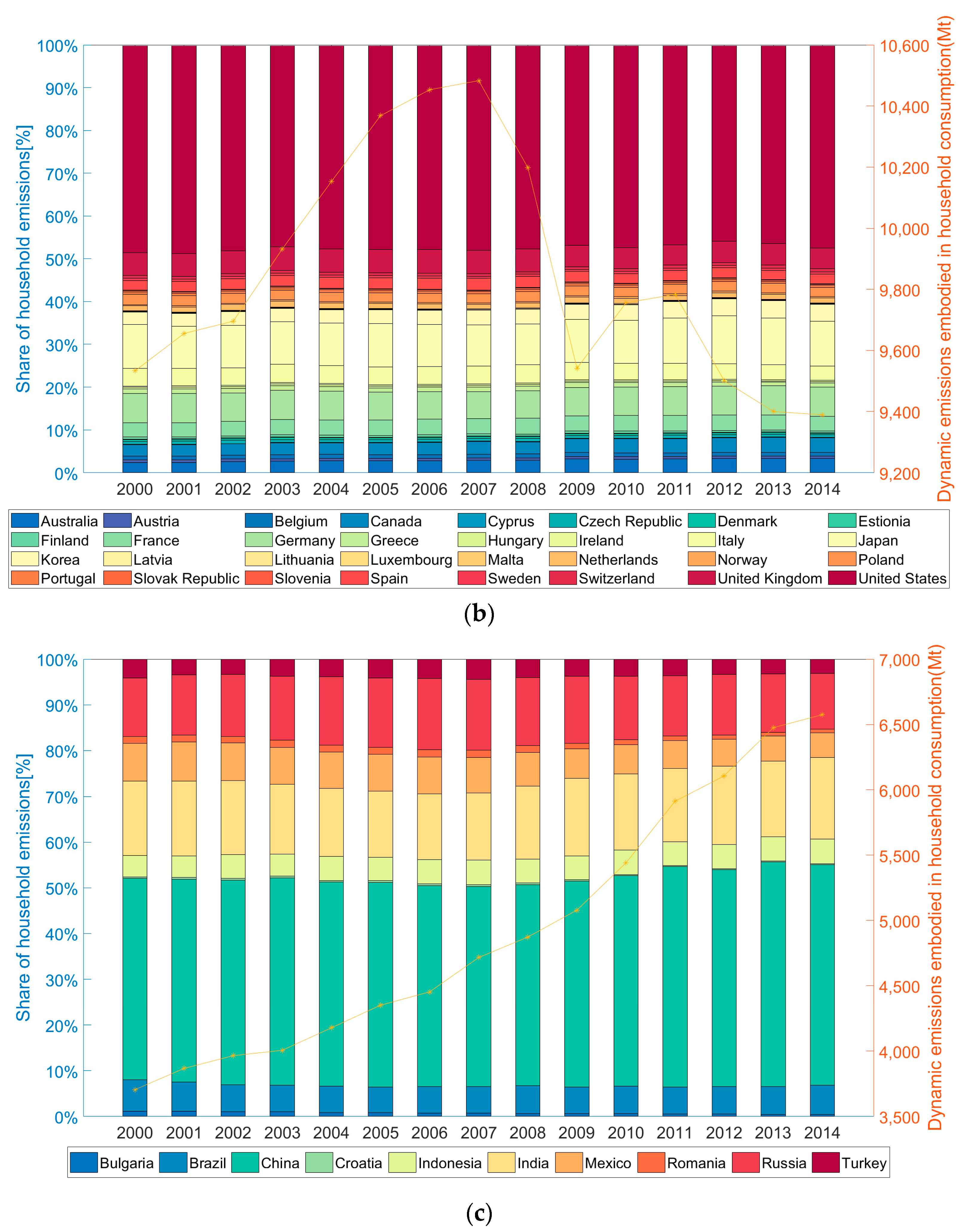
This study examined and compared the traditional and dynamic embodied carbon emissions of households worldwide in both developed and developing countries, which were shown in Figure 1. Whether looking globally, or at specific developed/developing countries, the dynamic embodied carbon emissions of households consistently exceed their traditional embodied carbon emissions. This is because the traditional model does not account for implicit carbon emissions included in capital inputs and does not consider the temporal deviation between current consumption and future emissions owing to changes in capital stock [10]. This results in an underestimation of the carbon footprint. In 2014, the proportion of embodied carbon emissions underestimated by traditional models was 24.02% and 26.03% of the carbon footprint of households in developed and developing countries, respectively. This highlights the importance of re-estimating household carbon footprints using dynamic models, particularly in developing countries during periods of rapid capital accumulation.

From 2000 to 2014, both direct and embodied carbon emissions in developing countries exhibited continuous upward trends. Specifically, the dynamic embodied carbon emissions of households increased from 3704.98 Mt to 6574.25 Mt, while traditional embodied carbon emissions of households rose from 3164.56 Mt to 5216.26 Mt. In contrast, the trend of direct and embodied carbon emissions in developed countries was slightly different. Direct carbon emissions continued to decline, while embodied carbon emissions initially rose and then fell. This suggests that in the early stages of carbon emission reduction, developed countries transferred carbon emissions to other regions by importing products with high embodied carbon emissions, leading to the illusion of lower direct carbon emissions. The peak of traditional embodied carbon emissions occurred in 2005 at 8679.21 Mt, and the peak of dynamic embodied carbon emissions occurred in 2007 at 10,483.18 Mt. The difference between the two is due to the time shift caused by carbon emissions stored in fixed capital.

We calculated embodied carbon emissions of economies and showed the results in Figure 2. In terms of total embodied carbon emissions, the US has remained the top emitter, followed by China, the EU, India, and Japan in second to fifth positions, respectively. The rankings of each economy fluctuated slightly over the 15-year period; however, the changes were not significant. Moreover, the rankings of the countries differ significantly when embodied carbon emissions per capita are considered. The US maintains its position as the top emitter, but China, the European Union, and India experience significant declines in their rankings, dropping to the 12th, 8th, and 15th rankings, respectively. In contrast, developed countries such as Australia, Switzerland, and Canada move up in their rankings. Nevertheless, these countries appear to have achieved “low-carbon” development because of their small population sizes. Conversely, the high emissions in countries with large populations, such as China and India, are largely attributed to their large population bases, and these countries face greater pressure to reduce their emissions from residential consumption.

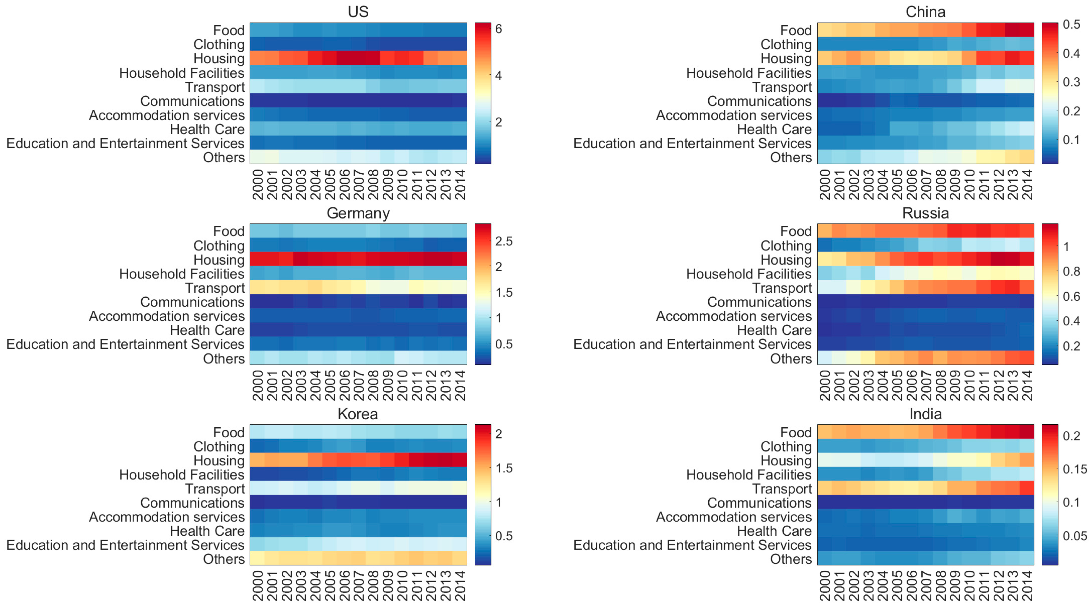
Significant differences exist in the embodied carbon emissions from household consumption categories between developed and developing countries, which were shown in Figure 3. Food consumption was the category with the highest share of embodied carbon emissions in developing countries, and the Engel coefficient of carbon emissions from households (i.e., the ratio of embodied carbon emissions from food consumption to total embodied carbon emissions from household consumption) remained above 20% from 2000 to 2014. Additionally, the share of embodied carbon emissions in categories such as clothing and household facilities was higher in developing countries than in developed countries. In developing countries, basic living needs are the most significant sources of households’ carbon footprint, and Engel’s coefficient of carbon emissions shows a decreasing trend as households’ living standards and disposable income increase. The different income levels, consumption habits, and consumption patterns of residents in each country, as well as the domestic industrial structure and product quantity and quality, cause differences in the consumption structures of each country. These differences have resulted in different structures of the embodied carbon footprints of residents’ consumption.

In developed countries, housing consumption had the highest share of embodied carbon emissions, which remained at approximately 30% throughout the 15 years. This is in contrast to developing countries, where the share was only approximately 20%. The share of embodied carbon emissions from transportation, household facilities, and healthcare was also higher in developed countries than in developing countries.

Each country has unique characteristics in terms of consumption categories, in addition to common trends, which were shown in Figure 4. For instance, China has a lower share of embodied carbon emissions from transportation consumption than other countries, with the highest share reaching only 10.24%, indicating success in achieving low-carbon travel. However, China’s share of embodied carbon emissions from healthcare, education, and entertainment services has increased significantly faster than that of other countries, reflecting the changing consumption structure due to economic development and rising living standards. Germany, South Korea, and India have had little change in the structure of households’ dynamic carbon footprints over the past 15 years. In the US, the share of household carbon emissions rose and then fell, with the turning point occurring around 2008, reflecting the impact of the financial crisis on residential consumption.

4.2. Decomposition Analysis of Changes in Total Carbon Footprint

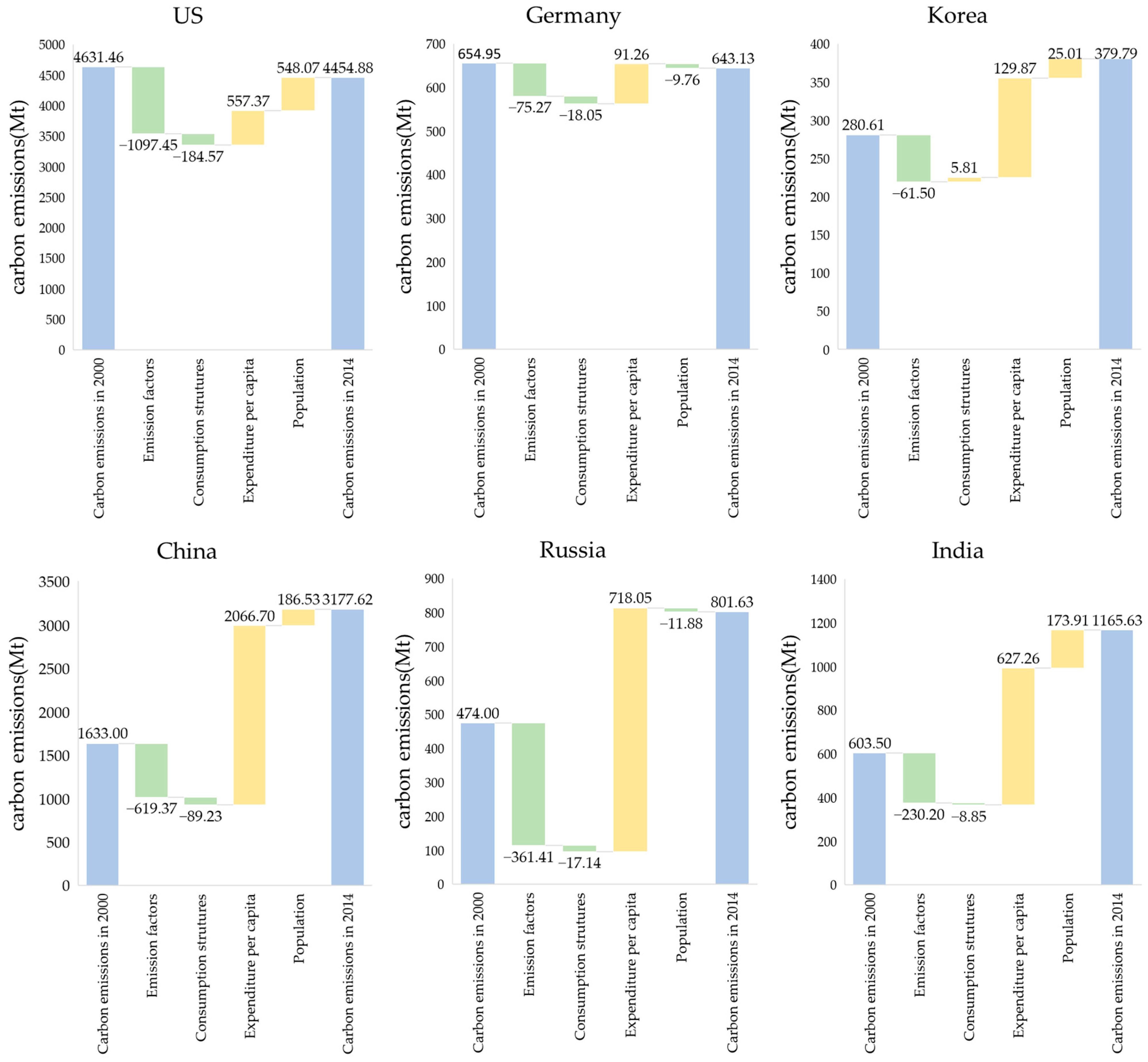
To further investigate the factors driving the changes in carbon footprint between 2000 and 2014, an LMDI decomposition analysis was conducted, and the results were shown in Figure 5. The US and Germany saw a decrease in total carbon emissions, whereas China, Russia, India, and South Korea all experienced an increase. The emission intensity effect had a similar impact in all countries, resulting in a reduction in the residential carbon footprint. In contrast, the consumption level effect had the opposite effect, contributing to an overall increase in the carbon footprint for all countries. This effect emerged as the primary driver of carbon emission growth due to increased household consumption. In addition, the consumption structure effect had a mixed impact on carbon emissions across different countries. Finally, the population size effect was positive for all countries except Germany and Russia, which is consistent with the change in population size over the 15-year period.

China, South Korea, and India experienced much greater increases in carbon emissions because of the consumption level effect rather than the population size effect. Conversely, in the US, both effects contributed almost equally to carbon emissions increasing. Additionally, the consumption structure effect resulted in a reduction in carbon emissions for all countries except South Korea. This reduction was particularly significant in the US and Germany, reaching 104.53% and 152.70%, respectively.

4.3. Decomposition Analysis of Change into Category and Structural Components

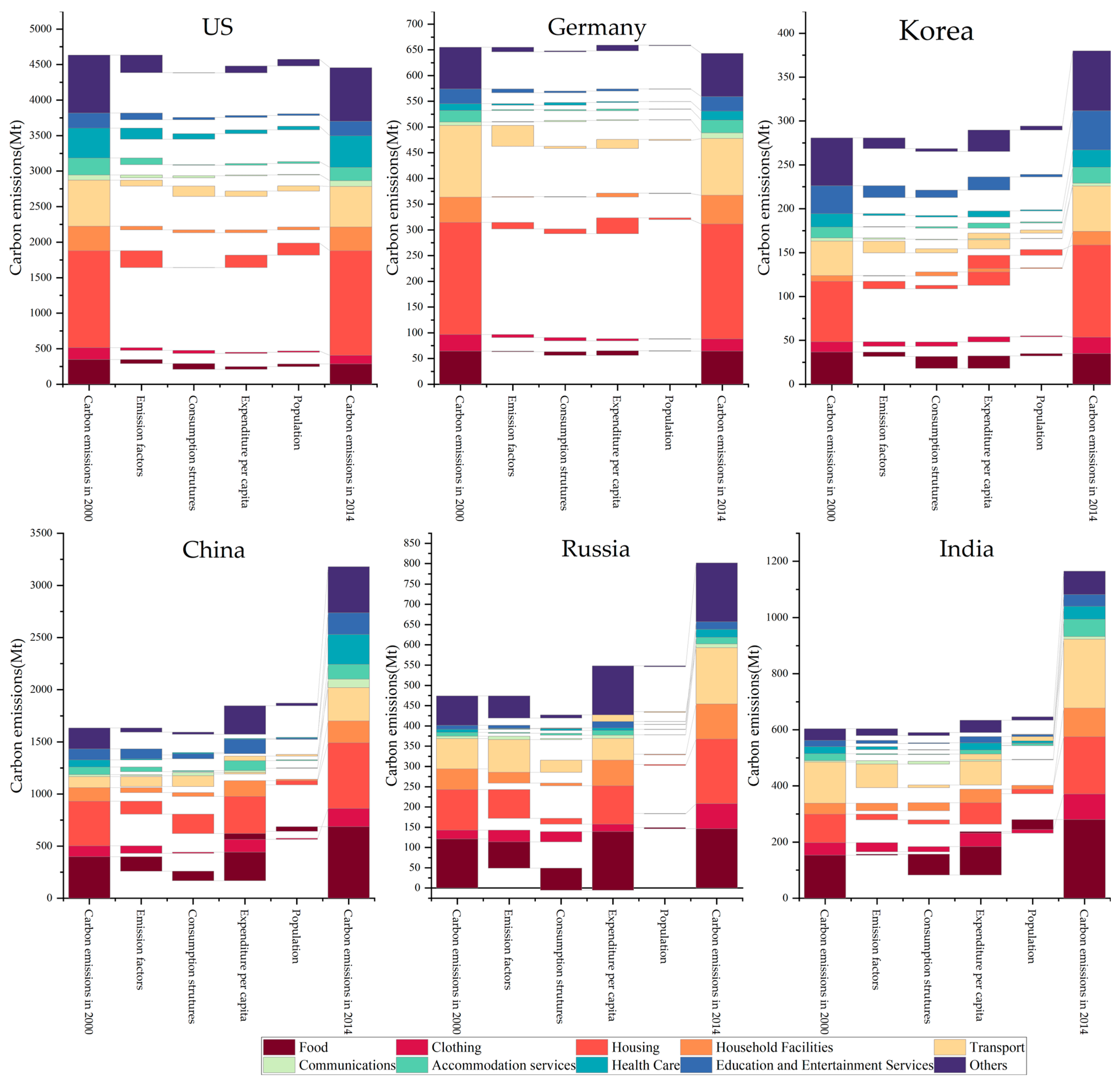
To further explore the impact of each consumption category, we conducted an LMDI analysis of the consumption in different categories and the results were shown in Figure 6. The carbon footprints of China, Russia, and India increased in all categories, whereas the US, Germany, and South Korea achieved carbon reductions in seven, three, and two consumption categories, respectively. For China, the five categories that showed the highest increase in carbon emissions were food, other goods and services, healthcare, transportation, and housing, all of which increased by more than 200 Mt over the 15 years. These five categories also accounted for the largest share of the carbon footprint of Chinese residential consumption in 2014. Therefore, to reduce emissions in the residential sector, it is essential to control the carbon emissions of these five categories. In the US, residential carbon emission reductions have been achieved in seven categories: transportation, food, other goods and services, accommodation services, clothing, education, culture and entertainment services, and household equipment supplies and services.

The emissions intensity effect is generally the strongest contributor to changes in carbon emissions across most consumer categories, although its impact varies by country. For example, in the US, the emission intensity effect contributed the most to carbon reduction from education consumption, with a reduction contribution of 854.31%. In contrast, in China, this effect achieved a much lower contribution of only 99.34% and its absolute impact was relatively low, making it impossible to counterbalance the carbon increase resulting from other effects, especially the consumption level effect.

The effect of consumption structure on carbon emissions varies significantly across consumption categories. In China, it reduced carbon emissions in housing, food, household equipment and services, and other goods and services, whereas it triggered an increase for other categories. Similarly, consumption structure resulted in an increase in carbon emissions in most consumption categories in Russia, India, and South Korea, and the absolute carbon reduction was small and insufficient to offset this. In contrast, in the US and Germany, which achieved total carbon emission reduction, the consumption structure effect caused a carbon reduction effect in most categories, with the exception of communication, education, and healthcare. The consumption structure and the emission intensity effects were almost the same in terms of carbon reduction, and the carbon reduction effect of the consumption structure effect exceeded that of the emission intensity effect.

5. Discussion

5.1. Differences in Household Carbon Footprint in Developing and Developed Countries

This study further highlights significant variations between developed and developing countries in the carbon footprints of household consumption categories. Consumption structures and the intensity of embodied carbon emissions vary between economies. For instance, in 2014, the embodied carbon emission intensity of food in developing countries was 1.22, which was twice as high as that in developed countries (0.66). Consequently, the proportion of food consumption in developing countries was as high as 21.82%, which was more than twice that of developed countries (6.99%). Differences in carbon emission categories have significant implications for changes in carbon emissions across countries. For instance, in China, the transportation, food, and other goods and services categories have witnessed a significant increase in carbon emissions over the last 15 years, while the US has achieved considerable carbon emission reductions in these categories. This discrepancy leads to varying trends in carbon emissions between developed and developing countries. To achieve carbon emission reductions, developing countries such as China must focus on reducing the embodied carbon emissions of basic needs such as food, clothing, housing, and transportation.

In addition to differences in emission categories, there are variations in the drivers of emission changes between different countries. For instance, while emission intensity reduction is the most critical factor in China, its reduction rate is lower than that of the US and Germany, at 621.50% and 636.70%, respectively. Therefore, China can learn from the advanced experiences of other countries and focus on promoting emission reduction and energy-saving technologies and improving energy efficiency.

Furthermore, consumption structures and emission intensity contributed 5.78% and 40.10%, respectively, to carbon reduction in China. The contribution of the consumption structure effect is negligible compared with the other three effects. Although China’s consumption structure reduced carbon emissions, the change was minimal. The most significant factor was the emission intensity effect, which represents the dynamic carbon footprint corresponding to a unit of residential consumption. Its contribution represents a reduction in the production process, including the use of clean energy, carbon sequestration technologies, resource conservation, and green technological innovations.

It is also interesting to note that for most consumption categories, the emission intensity effect triggered different levels of carbon reduction. However, in China and Russia, the emission intensity effect leads to an increase in the carbon footprint of healthcare consumption. Economic development has improved people’s lives, but it also causes environmental problems such as air pollution, water pollution, and the greenhouse effect. These problems lead to an increase in healthcare expenditure. Moreover, the carbon emission intensity of healthcare consumption increased between 2000 and 2014, further exacerbating the greenhouse effect. The healthcare sector is a significant source of greenhouse gases [47], and the rising carbon intensity of healthcare consumption has made it more challenging to reduce residential emissions. To address this issue, it is necessary to promote low-carbon healthcare operations, establish a low-carbon healthcare system, and reduce the carbon intensity of the healthcare sector through clean renewable energy substitution, the establishment of recycling systems, efficient pollutant disposal, and the use of reasonable carbon capture technologies.

5.2. Policy Implications for Shifts in Carbon Emissions

Based on these findings, countries should consider their specific consumption characteristics when formulating carbon reduction policies for residential sectors. In developing countries, focusing on reducing emissions from housing, food, and transportation can lead to significant reductions as these categories account for more than half of the total consumption carbon emissions. Therefore, encouraging low-carbon patterns in these areas can be effective.

Reducing carbon emission intensity during production processes is also a powerful way to reduce residential carbon emissions. Improving energy efficiency, increasing the use of clean energy, and investing in green innovation and carbon capture technologies can help reduce the embodied carbon emission intensity. Additionally, reducing the input of high-emission intermediate goods can reduce carbon emission intensity.

Changes in consumption structure can also contribute to reducing the carbon footprint. Reducing consumption in high-carbon intensity categories and increasing consumption in low-carbon intensity categories can help offset the carbon footprint increase due to population growth and consumption levels.

Given the pressure of a large population and rapidly increasing consumption levels, reducing emission intensity and changing consumption structures with a dual approach is necessary to achieve carbon reduction in the residential sector. In addition to strictly managing direct carbon emissions from industrial production processes, the government should introduce policies to encourage residents to reduce their consumption of products with high carbon emission intensities.

6. Conclusions

This study employed a dynamic input–output model to accurately assess the global carbon footprint and applied LMDI decomposition analysis to investigate the key drivers of residential carbon emissions across various countries. Direct carbon emissions fail to account for the regional transfer of carbon emissions, and the traditional accounting methods ignore the temporal transfer of carbon emissions. Hence, it is necessary to re-estimate residents’ carbon footprints using dynamic models.

The analysis revealed substantial differences between developed and developing countries in terms of the carbon footprint of residential consumption categories and their driving forces, leading to divergent trends in household carbon footprints. The impacts of population size, consumption level, and emission intensity were consistent across countries, while consumption structure effects varied. For most countries, an increase in residential consumption expenditure was the most important reason for the increase in carbon emissions, whereas a decrease in carbon emission intensity was the biggest driver for countries to reduce carbon emissions.

In developing countries, the absolute emission intensity effect is lower, and the consumption structure effect of most consumption categories leads to an increase in carbon emissions. Additionally, the absolute amount of carbon reduction in sectors that achieve carbon reduction is smaller, making it difficult to offset the increase in carbon emissions due to the increase in consumption expenditure and population growth. Therefore, countries must focus on improving their consumption structure and reducing the emission intensity of high-carbon-emitting consumption categories to decrease carbon emissions. It is essential for all countries to prioritize reducing the emission intensity and transforming consumption patterns to effectively address the challenge of reducing carbon emissions. Compared to developed countries such as the US and Germany, these efforts are even more crucial for developing countries.

This research has some limitations, leaving open various directions that future researchers could explore. Firstly, using data that are more updated or detailed to account for residents’ carbon footprint may uncover new features and changes through longer time series. Secondly, considering international trade factors in the LMDI decomposition analysis by distinguishing between the consumption of domestic and imported goods could improve our understanding of the drivers behind residential carbon footprints. Lastly, the inclusion of residents’ characteristics, such as income or education level, would allow for a detailed investigation into the heterogeneity of their carbon emissions.

References

1. Li, Y.; Zhang, H. Regional differences in the effects of urbanization on household CO2 emissions: An analysis based on provincial panel data in China. Resour. Sci. 2016, 38, 545–556. [Google Scholar]
2. Cao, X.; Gao, Y.; Liu, Z. Analysis of the impact of urbanization of rural population on carbon emissions of residential energy consumption. Chin. Rural Econ. 2021, 10, 64–83. [Google Scholar]
3. Brizga, J.; Feng, K.; Hubacek, K. Household carbon footprints in the Baltic States: A global multi-regional input–output analysis from 1995 to 2011. Appl. Energy 2017, 189, 780–788. [Google Scholar] [CrossRef]
4. Kurniawan, R.; Sugiawan, Y.; Managi, S. Cleaner energy conversion and household emission decomposition analysis in Indonesia. J. Clean. Prod. 2018, 201, 334–342. [Google Scholar] [CrossRef]
5. Peng, S.; Zhang, W.; Sun, C. Measurement of carbon emissions and influencing factors on production and consumption in China. Econ. Res. J. 2015, 50, 168–182. [Google Scholar]
6. Chen, Z.M.; Chen, P.; Lenzen, M.; Xiao, B.; Malik, A. Global Embodied Energy Flow and Stock Analysis with Endogeneous Fixed Capital. Environ. Sci. Technol. 2022, 56, 17197–17205. [Google Scholar] [CrossRef]
7. Zhang, Y.; Shen, L.; Shuai, C.; Tan, Y.; Ren, Y.; Wu, Y. Is the low-carbon economy efficient in terms of sustainable development? A global perspective. Sustain. Dev. 2019, 27, 130–152. [Google Scholar] [CrossRef]
8. Wang, Q.; Zhou, Y. Evolution and drivers of production-based carbon emissions in China and India: Differences and similarities. J. Clean. Prod. 2020, 277, 123958. [Google Scholar] [CrossRef]
9. Bin, S.; Dowlatabadi, H. Consumer lifestyle approach to US energy use and the related CO2 emissions. Energy Policy 2005, 33, 197–208. [Google Scholar] [CrossRef]
10. Chen, Z.M.; Ohshita, S.; Lenzen, M.; Wiedmann, T.; Jiborn, M.; Chen, B.; Lester, L.; Guan, D.; Meng, J.; Xu, S.; et al. Consumption-based greenhouse gas emissions accounting with capital stock change highlights dynamics of fast-developing countries. Nat. Commun. 2018, 9, 3581. [Google Scholar] [CrossRef]
11. IPCC. 2019 Refinement to the 2006 IPCC Guidelines for National Greenhouse Gas Inventories; IPCC: Geneva, Switzerland, 2019. [Google Scholar]
12. IPCC. 2006 IPCC Guidelines for National Greenhouse Gas Inventories; IPCC: Geneva, Switzerland, 2006. [Google Scholar]
13. Liu, Z.; Guan, D.; Wei, W.; Davis, S.J.; Ciais, P.; Bai, J.; Peng, S.; Zhang, Q.; Hubacek, K.; Marland, G.; et al. Reduced carbon emission estimates from fossil fuel combustion and cement production in China. Nature 2015, 524, 335–338. [Google Scholar] [CrossRef] [PubMed]
14. Rocco, M.V.; Golinucci, N.; Ronco, S.M.; Colombo, E. Fighting carbon leakage through consumption-based carbon emissions policies: Empirical analysis based on the World Trade Model with Bilateral Trades. Appl. Energy 2020, 274, 115301. [Google Scholar] [CrossRef]
15. Zhang, X.; Luo, L.; Skitmore, M. Household carbon emission research: An analytical review of measurement, influencing factors and mitigation prospects. J. Clean. Prod. 2015, 103, 873–883. [Google Scholar] [CrossRef]
16. Jones, C.M.; Kammen, D.M. Quantifying Carbon Footprint Reduction Opportunities for US Households and Communities. Environ. Sci. Technol. 2011, 45, 4088–4095. [Google Scholar] [CrossRef] [PubMed]
17. Ding, Q.; Cai, W.; Wang, C.; Sanwal, M. The relationships between household consumption activities and energy consumption in china—An input-output analysis from the lifestyle perspective. Appl. Energy 2017, 207, 520–532. [Google Scholar] [CrossRef]
18. Druckman, A.; Jackson, T. The carbon footprint of UK households 1990–2004: A socio-economically disaggregated, quasi-multi-regional input-output model. Ecol. Econ. 2009, 68, 2066–2077. [Google Scholar] [CrossRef]
19. Machado, G.; Schaeffer, R.; Worrell, E. Energy and carbon embodied in the international trade of Brazil: An input-output approach. Ecol. Econ. 2001, 39, 409–424. [Google Scholar] [CrossRef]
20. Wiedmann, T.; Wood, R.; Minx, J.C.; Lenzen, M.; Guan, D.; Harris, R. Carbon footprint time series of the UK—Results from a multi-region input-output model. Econ. Syst. Res. 2010, 22, 19–42. [Google Scholar] [CrossRef]
21. Alfredsson, E.C. “Green” consumption—No solution for climate change. Energy 2004, 29, 513–524. [Google Scholar] [CrossRef]
22. Saner, D.; Heeren, N.; Jäggi, B.; Waraich, R.A.; Hellweg, S. Housing and mobility demands of individual households and their life cycle assessment. Environ. Sci. Technol. 2013, 47, 5988–5997. [Google Scholar] [CrossRef]
23. Zhang, L.X.; Wang, C.B.; Song, B. Carbon emission reduction potential of a typical household biogas system in rural China. J. Clean. Prod. 2013, 47, 415–421. [Google Scholar] [CrossRef]
24. Wang, Z.; Yang, L. Indirect carbon emissions in household consumption: Evidence from the urban and rural area in China. J. Clean. Prod. 2014, 78, 94–103. [Google Scholar] [CrossRef]
25. Wei, Y.M.; Liu, L.C.; Fan, Y.; Wu, G. The impact of lifestyle on energy use and CO2 emission: An empirical analysis of China’s residents. Energy Policy 2007, 35, 247–257. [Google Scholar] [CrossRef]
26. Pauliuk, S.; Wood, R.; Hertwich, E.G. Dynamic Models of Fixed Capital Stocks and Their Application in Industrial Ecology. J. Ind. Ecol. 2015, 19, 104–116. [Google Scholar] [CrossRef]
27. Cao, Q.; Kang, W.; Xu, S.; Sajid, M.J.; Cao, M. Estimation and decomposition analysis of carbon emissions from the entire production cycle for Chinese household consumption. J. Environ. Manag. 2019, 247, 525–537. [Google Scholar] [CrossRef]
28. Ding, Y.; Li, F. Examining the effects of urbanization and industrialization on carbon dioxide emission: Evidence from China’s provincial regions. Energy 2017, 125, 533–542. [Google Scholar] [CrossRef]
29. Zang, X.; Zhao, T.; Wang, J.; Guo, F. The effects of urbanization and household-related factors on residential direct CO2 emissions in Shanxi, China from 1995 to 2014: A decomposition analysis. Atmos. Pollut. Res. 2017, 8, 297–309. [Google Scholar] [CrossRef]
30. Das, A.; Paul, S.K. CO2 emissions from household consumption in India between 1993–94 and 2006–07: A decomposition analysis. Energy Econ. 2014, 41, 90–105. [Google Scholar] [CrossRef]
31. Wang, W.; Kuang, Y.; Huang, N. Study on the decomposition of factors affecting energy-related carbon emissions in Guangdong province, China. Energies 2011, 4, 2249–2272. [Google Scholar] [CrossRef]
32. Guo, W.; Sun, T. The Impact of Population Structure Changes on Carbon Emissions from Energy Consumption in China—Based on the Perspective of Urbanization and Resident Consumption. J. Appl. Stat. Manag. 2017, 36, 295–312. [Google Scholar]
33. Zhu, Q.; Wei, T. The impact of population urbanization on carbon emissions from the perspective of household consumption. China Popul. Resour. Environ. 2013, 23, 21–29. [Google Scholar]
34. Du, W. Analysis of indirect carbon emissions from Chinese residents based on LMDI decomposition model. China Popul. Resour. Environ. 2016, 26, 5–9. [Google Scholar]
35. Kulionis, V.; Wood, R. Explaining decoupling in high income countries: A structural decomposition analysis of the change in energy footprint from 1970 to 2009. Energy 2020, 194, 116909. [Google Scholar] [CrossRef]
36. Araújo IF, D.; Jackson, R.W.; Ferreira Neto, A.B.; Perobelli, F.S. European union membership and CO2 emissions: A structural decomposition analysis. Struct. Chang. Econ. Dyn. 2020, 55, 190–203. [Google Scholar] [CrossRef]
37. Xie, R.; Wang, F.; Chevallier, J.; Zhu, B.; Zhao, G. Supply-side structural effects of air pollutant emissions in China: A comparative analysis. Struct. Chang. Econ. Dyn. 2018, 46, 89–95. [Google Scholar] [CrossRef]
38. Timmer, M.P.; Dietzenbacher, E.; Los, B.; Stehrer, R.; de Vries, G.J. An Illustrated User Guide to the World Input-Output Database: The Case of Global Automotive Production. Rev. Int. Econ. 2015, 23, 575–605. [Google Scholar] [CrossRef]
39. Adarov, A.; Stehrer, R. Tangible and Intangible Assets in the Growth Performance of the EU, Japan and the US; WIIW: Vienna, Austria, 2019. [Google Scholar]
40. Stehrer, R.; Bykova, A.; Jäger, K.; Reiter, O.; Schwarzhappel, M. Industry Level Growth and Productivity Data with Special Focus on Intangible Assets; WIIW: Vienna, Austria, 2019. [Google Scholar]
41. Kaya, Y. Impact of Carbon Dioxide Emission Control on GNP Growth: Interpretation of Proposed Scenarios; IPCC: Geneva, Switzerland, 1990. [Google Scholar]
42. Ang, B.W.; Zhang, F.Q.; Choi, K.H. Factorizing changes in energy and environmental indicators through decomposition. Energy 1998, 23, 489–495. [Google Scholar] [CrossRef]
43. Ang, B.W. The LMDI approach to decomposition analysis: A practical guide. Energy Policy 2005, 33, 867–871. [Google Scholar] [CrossRef]
44. Wang, B.; Sun, Y.; Chen, Q.; Wang, Z. Determinants analysis of carbon dioxide emissions in passenger and freight transportation sectors in China. Struct. Chang. Econ. Dyn. 2018, 47, 127–132. [Google Scholar] [CrossRef]
45. Wang, Z.; Liu, W.; Yin, J. Driving forces of indirect carbon emissions from household consumption in China: An input–output decomposition analysis. Nat. Hazards 2015, 75, 257–272. [Google Scholar] [CrossRef]
46. Yuan, R.; Rodrigues JF, D.; Wang, J.; Tukker, A.; Behrens, P. A global overview of developments of urban and rural household GHG footprints from 2005 to 2015. Sci. Total Environ. 2022, 806, 150695. [Google Scholar] [CrossRef] [PubMed]
47. Sherman, J.D.; MacNeill, A.; Thiel, C. Reducing pollution from the health care industry [Short Survey]. JAMA-J. Am. Med. Assoc. 2019, 322, 1043–1044. [Google Scholar] [CrossRef] [PubMed]
Figure 1. Global direct carbon emissions, household direct carbon emissions, household traditional household carbon emissions, and household dynamic household carbon emissions, 2000–2014. (a) Total carbon emissions; (b) carbon emissions per capita. Direct carbon emissions data from EA accounts of WIOD (2016 version).
Energies 16 03884 g001aEnergies 16 03884 g001b
Figure 2. Dynamic embodied carbon emissions of households in economies worldwide in 2014. (a) All economies; (b) developed countries; (c) developing countries.
Energies 16 03884 g002aEnergies 16 03884 g002b
Figure 3. Dynamic embodied carbon emissions from global household consumption by category in 2014.
Energies 16 03884 g003
Figure 4. Dynamic embodied carbon emissions from various consumption categories of households in six countries from 2000 to 2014, with the unit of the vertical axis being Mt. Due to the length of the paper and the comparability between countries, only the results from the US, Germany, South Korea, China, Russia, and India are displayed in the figure.
Energies 16 03884 g004
Figure 5. The LMDI results of residents’ carbon footprints in six countries from 2000 to 2014. The purple bars represent the total carbon footprint from residents’ consumption in 2000 and 2014. The emission intensity effect, consumption structure effect, consumption level effect, and population size effect are represented by the bars labeled “Emission factors”, “Consumption structures”, “Expenditure per capita”, and “Population”, respectively. Yellow indicates that the effect increases carbon emissions, while green stands for reduction.
Energies 16 03884 g005
Figure 6. The LMDI results of the carbon footprint of residents’ consumption by category in six countries from 2000 to 2014. The purple bars represent the total carbon footprint. “Emission factors”, “Consumption structures”, “Expenditure per capita”, and “Population” represent the amount of carbon emission change due to these factors. Columns above the baseline show an increase in carbon emission, while columns below the baseline show a decrease.
Energies 16 03884 g006