Abstract
In recent years, time series forecasting has become an essential tool for stock market analysts to make informed decisions regarding stock prices. The present research makes use of various exponential smoothing forecasting methods. These include exponential smoothing with multiplicative errors and additive trend (MAN), exponential smoothing with multiplicative errors (MNN), and simple exponential smoothing with additive errors (ANN) for the forecasting of the stock prices of six different companies in the petroleum, electricity, and gas industries that are listed in the IBEX35 index. The database employed for this research contained the IBEX35 index values and stock closing prices from 3 January 2000 to 30 December 2022. The models trained with this data were employed in order to forecast the index value and the closing prices of the stocks under study from 2 January 2023 to 24 March 2023. The results obtained confirmed that although none of the proposed models outperformed the rest for all the companies, it is possible to calculate forecasting models able to predict a 95% confidence interval about real stock closing values and where the index will be in the following three months.
1. Introduction
In recent years, a worldwide rise in energy prices has been observed. This rise has been affected by both the COVID-19 pandemic and the Russian invasion of Ukraine [1]. In the case of the European Union, the Europe 2020 Strategy to promote smart, sustainable, and inclusive growth, the Green Deal [2], and the Sustainable Development Goals [3] have also impacted energy prices [4]. There are studies that confirm how both the COVID-19 pandemic and the Russian invasion of Ukraine have influenced the rise of energy prices [4] but have not significantly changed the European Union energy policies, which continue to promote the exploitation of renewable energy resources and support the improvement of energy efficiency systems to reduce climate polluting emissions.
In this context, among the main characteristics of global energy markets are price volatility and instability of development [5]. At the same time, macroeconomic data points out that a global recession in the second semester of 2023 [6] would be possible, but not sure. A recession like the one predicted would have a serious impact on some Western economies like Spain, which have already suffered seriously due to the financial crisis of 2007 [7,8], whose main consequences were a rise in unemployment and high levels of private debt [9].
Recent studies [10,11] have pointed out that despite the prevalence of common global factors affecting energy prices, local conditions such as tax regimes, energy sources, and demand also have great importance when it comes to fixing energy prices. In Spain, the energy sector has experienced a profound change in the last thirty years that has introduced markets and competition into the once-regulated monopolies of hydrocarbons, electricity, and gas. Within a complex international environment [12,13,14], the Spanish energy sector currently faces a transformation, but a necessary one if the goal of decarbonization is to be achieved.
In Spain, the most important companies in the energy sector that are publicly traded are included in the IBEX35. The IBEX35, an acronym for the Iberian Index, is the main stock market index in Spain. Nowadays, it is made up of the 35 largest companies by market capitalization. This is a weighted index like many others (i.e., SP500, FTSE 100), which means that not all companies have the same importance in it.
According to World Bank data [15], the market capitalization of all companies listed in 2020 in all the stock markets in the world was over 90 trillion US dollars. This large amount of money explains the current interest in the study of market dynamics. From the point of view of the weak version of the efficient-market hypothesis (EMH) [16,17], asset prices represent all the information that is currently known about past prices and disprove forecasts made based solely on price data. This implies that, according to such a theory, everyone who invests in stocks should be able to get the same return; as a result, nobody could outperform the market using technical analysis. It would not seem beneficial under these conditions to create strategies to anticipate the evolution of stock prices. Despite this concept and taking into account that this hypothesis would be false, many authors do not believe that markets are entirely efficient [18,19], especially considering phenomena such as their tendency to overreact in the short term [20,21]. Additionally, several of the key premises of the EMH have been shown to be false [22]. Considering these facts and the large amount of money present in the stock markets, the growing interest in the study of market dynamics and the creation of forecasting models makes sense.
In recent years, time series forecasting has become an essential tool for stock market analysts to make informed decisions regarding stock prices [22]. One of the significant benefits of using time series forecasting in the stock market is its ability to predict future stock prices. By analyzing historical data, analysts can identify patterns and trends in stock market behavior, which can help predict future stock prices [23]. This information can be used to make informed investment decisions, such as buying, selling, or holding a particular stock. Forecasting models can also help identify potential risks and opportunities in the market, allowing investors to adjust their investment strategies accordingly [23].
Another benefit of time series forecasting is its ability to identify long-term trends in the stock market [24]. By analyzing historical data over a more extended period, analysts can identify long-term trends in the market and use this information to develop long-term investment strategies [22].
Although time series forecasting is a valuable tool for predicting stock market trends, it does have its limitations. One of the most significant of these is that it relies on historical data, which may not be an accurate representation of future market behavior. The stock market is subject to many external factors, such as economic conditions, political events, and company-specific news, which can affect stock prices in unpredictable ways [22]. This means that historical data may not always be a reliable predictor of future trends.
Another limitation of time series forecasting is the potential for overfitting [25,26]. Overfitting occurs when a model is too closely fitted to historical data, leading to poor performance when new data is introduced. This can result in inaccurate predictions and investment decisions based on flawed data.
Therefore, time series forecasting is a valuable tool for predicting stock market trends and identifying potential investment opportunities [27]. Although it has its limitations, such as the reliance on historical data and the potential for overfitting, it remains an essential tool for investors and analysts.
The aim of the present study is to forecast the stock prices of IBEX35 companies in the petroleum, electricity, and gas industries, making use of time series methodologies. The purpose of this research is not only to develop forecasting models but also to analyze stock price dynamics under different market conditions. Due to the complexity of financial decisions in a changing environment, individuals who make them must consider several variables that require sophisticated mathematical models for their analysis [22]. Therefore, the fields of multivariate data analysis and machine learning have produced some of the most promising tools used in this undertaking. In the case of the present research, however, the study is limited to time series-based models. The present work focuses on the study of models based on time series given that they are, on the one hand, explainable models and, on the other, models in which only the price of the shares of the companies considered in the research will be taken into account for the forecast of future share prices. Please note that the main point of interest of this research is that, as far as the authors know, there is very little research that works with this kind of company [22].
This paper is organized as follows. After this introductory section, there is another in which the materials and methods employed in this study are described in detail. This section includes the database employed and the methodologies used for forecasting. After the description of the methodology, the results obtained for the forecasting of the time series are presented in the results section. Finally, an in-depth discussion is detailed in the discussion section.
2. Materials and Methods
This section includes the database employed in this research and also describes the methodologies used for forecasting.
2.1. The IBEX35 and the Companies under Study
The IBEX35 is a market capitalization-weighted index that tracks the performance of the 35 largest and most liquid Spanish stocks traded on the Bolsa de Madrid. Market capitalization is a measure of a company’s value, calculated by multiplying the number of outstanding shares by the current stock price. This index was launched on 14 January 1992, with a base value of 3000 points. It is calculated and published in real-time during trading hours and is used as a benchmark index for the Spanish equity market.
The makeup of the IBEX35 is reviewed twice a year, in June and December, with changes made based on market capitalization and liquidity criteria. The index is dominated by companies in the financial, energy, and telecommunications sectors, with some of the largest and most well-known Spanish companies, such as Banco Santander, Telefonica, and Repsol, featuring prominently.
Investors use the IBEX35 to track the performance of the Spanish equity market and to make investment decisions based on the index’s movements. Additionally, the IBEX35 can be used as a tool for portfolio diversification, allowing investors to gain exposure to a broad range of Spanish companies across multiple sectors. Overall, the IBEX35 is an important indicator of the Spanish economy’s health and provides a useful benchmark for investors seeking exposure to the Spanish equity market.
Table 1 shows all the companies that are part of IBEX35 in the second semester of 2022, including their relative weight in this index and the sector to which they belong. In the case of the present research, companies that belong to the electricity and gas, and petroleum sectors are studied. Those companies belonging to such sectors in IBEX35 are ENAGAS, ENDESA, IBERDROLA, NATURGY, RED ELECTRICA, and REPSOL. The sum weight of all these companies in the IBEX35 index is 21.88%, with weights ranging from 1.01% of ENAGAS to 12.4% of IBERDROLA.

Table 1.
Companies that belong to IBEX35 in the second semester of 2022 including their sector and weight in the index.
ENAGAS (Empresa Nacional del Gas) is a Spanish company founded in 1972. It is a company specializing in gas transport certified as Transmission System Operator (TSO) by the European Union, and it is also the owner of some regasification plants. Ninety percent of its stocks are free float. ENAGAS had featured in the IBEX35 since 2002, when it went public.
ENDESA (Empresa Nacional de Electricidad, S.A.) is a Spanish company founded in 1944. It was created as a state-owned company, and the sale of stocks and the company privatization was performed in 1988 when trading of stocks on the New York Stock Exchange started. Its main activities are currently electricity generation, distribution, commercialization, and also gas commercialization. Since the first quarter of 2009, ENDESA has been part of the ENEL Group (ente nazionale per l’energia elettrica), a multinational energy company based in Italy and a leading integrated operator in the world’s electricity and gas markets, focused on the European and Latin American markets.
IBERDROLA is a Spanish company founded in 1992 from the merger of two companies, Hidroeléctrica Española and Iberduero. This is the main energy group by market capitalization in the Spanish market, and its main activities are the production, distribution, and commercialization of electric energy. IBERDROLA is now one of the top five European electrical utilities in terms of stock market capitalization, with operations in dozens of countries on four continents.
NATURGY, whose legal name is Naturgy Energy Group S.A., is a Spanish company that works in the electric and gas markets. Although it was founded in 1991, the companies that merged to create NATURGY date back to the 19th Century.
Red Eléctrica Corporación S.A. is the company that operates the electric system in Spain, having more than 45,000 kms of power lines in service. It also has a presence in the international market and works as the operator of other electric networks in countries like Chile and Peru. Currently, it is also the owner of Hispasat, a company that operates telecommunication satellites.
REPSOL S.A. is a Spanish petrochemical and energy company based in Madrid (Spain). It was founded in 1987 after the merger of some petrochemical companies. It was previously a state-owned company but was privatized in 1989. Nowadays, it is a global company that operates in Asia, Africa, America, and Europe.
Figure 1, Figure 2, Figure 3, Figure 4, Figure 5 and Figure 6 show the stock closing prices of the six companies under study from 3 January 2000 to 30 December 2022, except in the case of ENAGAS (Figure 1), whose data starts on 26 June 2002. Figure 7 also shows the IBEX35 index closing prices from 3 January 2000 to 30 December 2022 of this index. Please note that the information used for the training of the models proposed in this article will be only that corresponding to these time series.
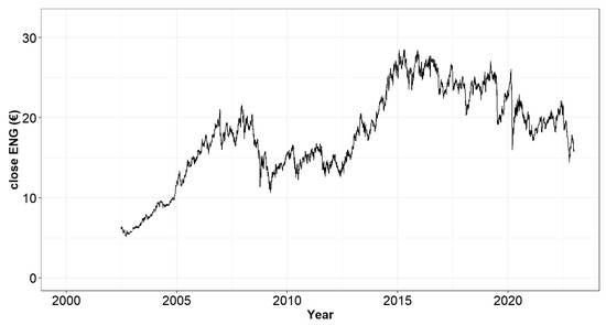
Figure 1.
ENAGAS stock closing prices from 26 June 2002 to 30 December 2022.
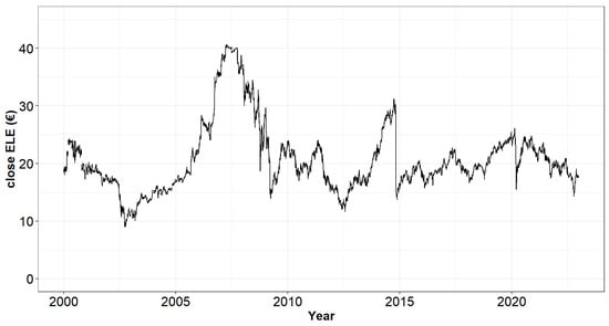
Figure 2.
ENDESA stock closing prices from 3 January 2000 to 30 December 2022.
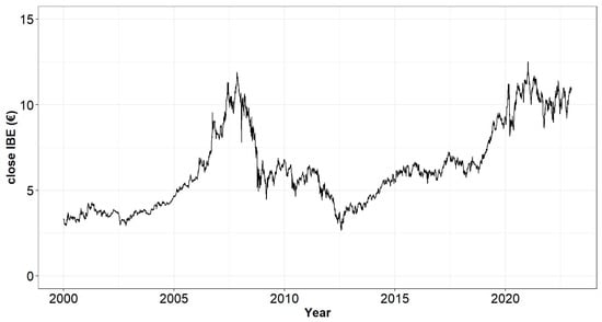
Figure 3.
IBERDROLA stock closing prices from 3 January 2000 to 30 December 2022.
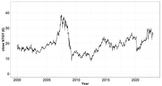
Figure 4.
NATURGY stock closing prices from 3 January 2000 to 30 December 2022.
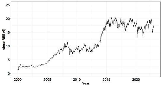
Figure 5.
RED ELECTRICA stock closing prices from 3 January 2000 to 30 December 2022.
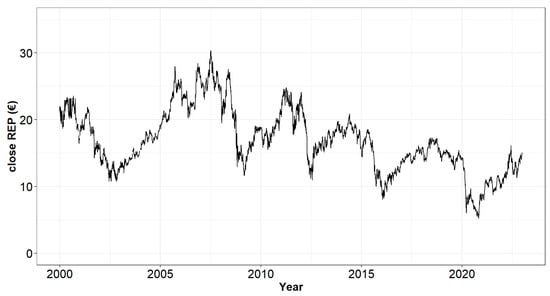
Figure 6.
REPSOL stock closing prices from 3 January 2000 to 30 December 2022.
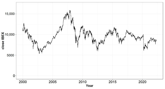
Figure 7.
IBEX35 index closing prices from 3 January 2000 to 30 December 2022.
In addition to the IBEX35, there are other indexes that are employed in the Spanish stock market. Some of the most widely followed indexes are as follows:
- IBEX Small Cap: This index is composed of the 30 most liquid small-cap companies listed on the Spanish stock market.
- IBEX Medium Cap: This index includes the 20 most liquid medium-cap companies listed on the Spanish stock market.
- IBEX Top Dividend: This index consists of the 10 highest dividend-yielding companies listed on the Spanish stock market.
- IBEX Growth Market: This index is made up of the 15 most innovative and fast-growing companies listed on the Spanish stock market.
- IBEX Net: This index is composed of the companies listed on the IBEX35 but with a modified weighting system that considers the companies’ free-float market capitalization.
All these indexes provide investors with different ways to track the performance of various segments of the Spanish stock market, allowing them to invest in a diversified range of companies based on their investment objectives and risk tolerance.
2.2. Smoothing Methods
Smoothing involves averaging values over multiple periods in order to reduce noise. Smoothing methods are data-driven and are able to adapt to changes in the series pattern over time [23]. One of the main drawbacks of this kind of method is that users must specify smoothing constants, which determine how fast methods adapt to new data.
A moving average consists of a window of consecutive periods, generating a series of averages. There are two kinds of moving averages [28]:
- Centered moving averages, which are powerful for visualizing trends.
- Trailing moving averages, which are powerful for visualizing trends because the averaging operation can suppress seasonality and noise, making the trend more visible.
The value of moving average at time is given by [28]:
where:
represents the window width and must be an odd number, and is the time at a certain point. The window width is chosen in order to suppress seasonality to better visualize the trend. Therefore, the windows should be as wide as a seasonal cycle.
Centered moving averages are computed by averaging across data both in the past and the future, and therefore, they cannot be used for forecasting. For forecasting purposes, a trailing moving average is employed. The k-step-ahead forecast is as follows:
Differencing is employed to remove trends and seasonal patterns from data [29]. It consists of taking the difference between two values. A means subtracting the value from periods back as follows: .
is useful for removing trends. Please also note that for quadratic and exponential trends, it would be useful to apply two or three times. Finally, for removing a seasonal pattern with , must be applied.
2.3. Simple Exponential Smoothing
Simple exponential smoothing is similar to forecasting with a moving average [30]. In this case, instead of taking a simple average over the most recent values, a weighted average of all past values is taken, decreasing in an exponential way.
Like the moving average, simple exponential smoothing should only be used for forecasting series that have neither trend nor seasonality [30]. The forecast at time of the exponential smoother is given by:
where is the smoothing constant that is a value in the interval 0 to 1.
Sometimes the exponential forecaster is written as follows:
where is the forecast error in .
The value of is fixed by the researcher and determines the rate of learning. The higher the value of , the faster the learning and the lower the influence of past measurements. In practice, typical values are in the range from to . The selection of must be cautious so as to avoid overfitting [31]. Please also note that the moving average and simple exponential are approximately equal if the window width of the moving average is equal to [31,32].
Finally, it must be highlighted that one of the main characteristics of exponential smoothing is its flexibility. Simple exponential smoothing works in the same way as the moving average, although it makes use of a weighted average of all past values in which the weight is reduced in the oldest past values. As is well-known in existing literature, simple exponential smoothing should only be used for forecasting series with no trend or seasonality whose components are first removed by means of differencing.
2.4. Series for Additive Trend
For a series that contains a trend, a kind of double exponential smoothing called Holt’s linear trend model may be employed. The trend in this model can change over time [28], and the local trend is estimated from the data. The ahead forecast is given by combining the level estimate at time , , and the trend estimate, which is assumed to be additive, at time .
The level and trend are updated through a pair of updating equations:
The first of the above and the level in the previous period adjusted for trend [33] is a weighted average of the trend in the previous period and the more recent information on the change in the level. Please also note that as and are the constants that determine the rate of learning, the value of both are and .
An exponential smoothing model [33,34] can capture two kinds of errors. The first is the additive error that can be expressed as follows:
where:
is the level at time
is the trend at time , and is the error at time .
In those cases in which the size of the error increases as the level of the series increases, a multiple active formula will be employed. Such a formula is given by:
The additive trend model assumes that the level changes from one period to the next by a fixed amount. In other words, exponential smoothing with a multiplicative trend produces forecast using the formula:
The updating equations for the level and trend are as follows:
In this model, an additive or multiplicative error can be included in the multiplicative trend mode. The additive error is given by:
While the multiplicative error is [34]:
2.5. Series with a Trend and Seasonality
In the case of a series with trend and seasonality, Holt–Winter’s exponential smoothing method may be employed [35,36]. In this model, the ahead forecast also considers the season at period .
Assuming seasonality with seasons, the forecast for an additive trend and multiplicative seasonality is given by:
This formula can only be applied if at least one full cycle of seasons is included in the forecasting time. In other words, .
In Holt–Winter’s exponential smoothing method, the level, trend, and seasonality patterns change over time. The updating equations for this model are given by:
The additive seasonality version of Holt–Winter’s exponential smoothing can be constructed from the multiplicative version by replacing multiplication and division signs by addition or subtraction signs from a seasonal component:
2.6. Models Employed in the Present Study
For the additive and multiplicative seasonality versions of the exponential smoothing model introduced previously, either an additive or multiplicative error can be included with an additive trend, a multiplicative trend, or no trend at all. This means that 18 different models are trained for each data set. These models have 2 different error types that can be multiplied by 3 different trend types and 3 different seasonality types.
The best-fitted models are those with the largest values of Akaike’s Information Criterion (AIC), Akaike’s Information Criterion Corrected (AICC), and Bayesian’s Information Criterion (BIC) [37]. One of the main characteristics of Akaike’s Information Criterion (AIC) is that it combines a fit to the training data with a penalty for the number of smoothing parameters and initial values included in the model. In other words, the AIC criterion penalizes a model for having a poor fit to the training period and for being more complicated, which is because simpler models can help avoid over-fitting and can improve predictions.
The BIC is also a statistical measure used for model selection. It provides a way to compare the fit of different statistical models to a given dataset while taking into account the number of parameters used in each model. It is based on Bayesian principles and is derived from the likelihood function of the model, adjusted for the number of parameters used. It balances the trade-off between model complexity (the number of parameters used) and the goodness-of-fit (how well the model fits the data).
3. Results
This section presents the results of applying the exponential smoothing method to the time series of the companies ENAGAS, ENDESA, IBERDROLA, NATURGY, RED ELECTRICA, and REPSOL, and also to the IBEX35 index. In all the cases, the period considered for the model training was from January 2000 to December 2022, with the exception of ENAGAS, whose time series data started in 2002, as was explained earlier.
Table 2 shows the correlation coefficients matrix of the companies under study and the IBEX35 index for the closure stock values from 3 January 2000 to 30 December 2022. As can be observed in this table, the strongest relationships of IBEX35 are with ENDESA (0.828) and REPSOL (0.734), followed by NATURGY (0.586). It is of interest to remark that despite the weight of these three companies in IBEX35 being under 3.5%, their correlation coefficient with IBEX35 is higher than that of IBERDROLA (0.330), whose weight in IBEX is 12.40%. Regarding relationships between companies, it is worth noting the high correlation between Red Eléctrica Corporación and ENAGÁS (0.913), NATURGY and ENDESA (0.704), NATURGY and IBERDROLA (0.695), and Red Eléctrica Corporación and IBERDROLA (0.601), while the rest of the positive correlations are all below 0.6. Regarding the negative correlations, the only notable ones are REPSOL and Red Eléctrica Corporación (−0.434) since all the others are below 0.2.
Table 2.
Correlation coefficients matrix of the companies under study and the IBEX35 index in the period under study (3 January 2000 to 30 December 2022). ENG: ENAGÁS, ELE: ENDESA, IBE: IBERDROLA, NTGY: NATURGY, REE: Red Eléctrica Corporación, REP: REPSOL.
With the help of the data available for each company, different exponential smoothing models were tested. These models made use of two different error types (‘additive’ or ‘multiplicative’), three trend types (‘no trend’, ’additive’, or ‘multiplicative’), and three kinds of season types (‘no seasonality’, ‘additive’, and ‘multiplicative’). For the additive models, Holt’s linear trend was employed, while in the case of the multiplicative ones, Holt–Winters’ method was the option selected.
One key decision when using exponential smoothing is whether to model the errors as additive or multiplicative. When using exponential smoothing with additive errors, it is assumed that the forecast error is constant across time periods, regardless of the magnitude of the forecast. This assumption implies that the forecast error is independent of the level of the time series. Conversely, exponential smoothing with multiplicative errors assumes that the forecast error is proportional to the level of the time series. In other words, the magnitude of the forecast error increases or decreases as the level of the time series does the same.
Therefore, the choice between additive and multiplicative errors depends on the characteristics of the time series being analyzed. Multiplicative errors are appropriate when the size of the error is likely to be proportional to the level of the time series. For instance, if the time series exhibits a trend, a change in the level of the series will result in a proportionate change in the size of the forecast error. Therefore, it is important to carefully consider the appropriate error model when using exponential smoothing for forecasting.
Exponential smoothing with multiplicative errors and additive trend assumes that the errors are proportional to the level of the time series, while the trend component is additive. In other words, the forecast error grows or shrinks proportionally with the level of the time series, while the trend component changes by a constant amount in each time period. This model is useful when the magnitude of the forecast error is likely to be proportional to the level of the time series and the time series exhibits a linear trend. On the other hand, exponential smoothing with additive errors and additive trends assumes that the errors are constant across time periods, regardless of the magnitude of the forecast, and the trend component is additive. In this model, the forecast error is assumed to be independent of the level of the time series, while the trend component changes by a constant amount in each time period. This model is appropriate when the magnitude of the forecast error is constant across time periods and the time series exhibits a linear trend.
The results obtained for the best exponential smooth models trained for each one of the companies under study and the IBEX35 index are detailed in Table 3. As can be observed, ENAGÁS and Red Eléctrica Corporación obtained the best fit with the MAN model, which means that the best fit of the stock closing prices of both companies is performed by exponential smoothing with multiplicative errors and the additive trend model. This means that recent data is more relevant to predicting future values than older data. This model has been found to be relevant in similar research, for instance, forecasting stock prices [38] and forecasting the growth of the Chinese economy [39].
Table 3.
Best exponential smooth model trained for each one of the companies under study and the IBEX35 index. MAN: exponential smoothing with multiplicative errors and additive trend; MNN: exponential smoothing with multiplicative errors; and ANN: simple exponential smoothing with additive errors. Alpha smoothing parameter (Alpha), Akaike Information Criterion (AIC), Akaike Information Criterion Corrected (AICC), and Bayesian Information Criterion (BIC). ENG: ENAGÁS, ELE: ENDESA, IBE: IBERDROLA, NTGY: NATURGY, REE: Red Eléctrica Corporación, REP: REPSOL.
In the case of the companies ENDESA, IBERDROLA, and NATURGY, the model that obtained the best fit was MNN, that is, exponential smoothing with multiplicative errors. This model is particularly useful when the variance of the errors changes over time and when the magnitude of the errors is proportional to the magnitude of the predicted value. This technique has been applied in various fields, such as finance, economics, and meteorology. For example, a study published in 2019 [40] used the multiplicative error model to forecast stock prices, while another study published in 2020 [41] applied the model to predict air quality in China.
There was another model that gave the best fit for REPSOL as well as for the IBEX35 index. It was ANN, which is simple exponential smoothing with additive errors. As has been explained before, this technique uses a single smoothing parameter to weigh the influence of past observations in predicting future values of a time series. In this model, the error term is assumed to follow an additive distribution. This kind of model is commonly used in various applications such as finance, economics, and meteorology. For instance, in a study published in 2021 [42], simple exponential smoothing with additive errors was used to forecast the demand for crude oil in China. Another study [43] used the model to forecast electricity demand in India.
After training the models of the six companies under study and the IBEX35, the models were employed to forecast the stock price closing values and the IBEX35 index in the period from 2 January 2023 to 24 March 2023. In other words, these models performed a forecast of the market up to 60 days in advance. The results obtained are presented in Figure 8, Figure 9, Figure 10, Figure 11, Figure 12, Figure 13 and Figure 14. Please note that different models were trained depending on the company under study.
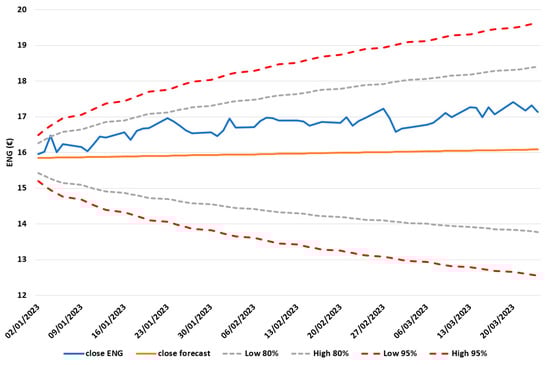
Figure 8.
ENG stock closing prices from 2 January 2023 to 24 March 2023. Closing values, forecasted closing values, and 80% and 95% confidence intervals of the forecasting of the exponential smoothing MAN model.
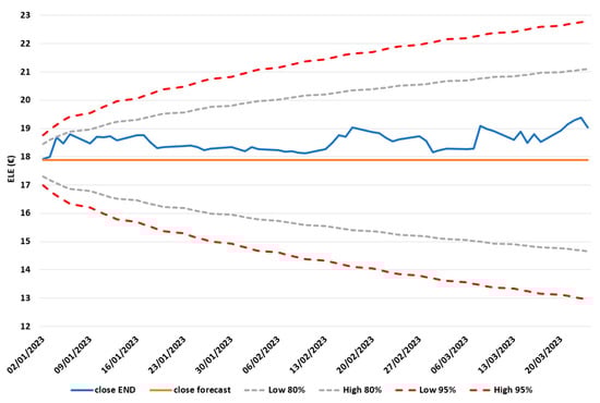
Figure 9.
ELE stock closing prices from 2 January 2023 to 24 March 2023. Closing values, forecasted closing values, and 80% and 95% confidence intervals of the forecasting of the exponential smoothing MNN model.
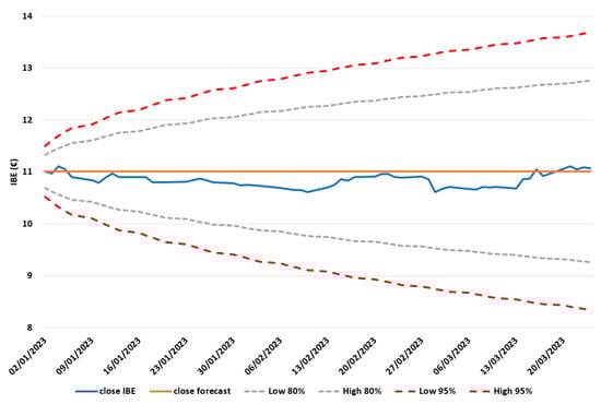
Figure 10.
IBE stock closing prices from 2 January 2023 to 24 March 2023. Closing values, forecasted closing values, and 80% and 95% confidence intervals of the forecasting of the exponential smoothing MNN model.
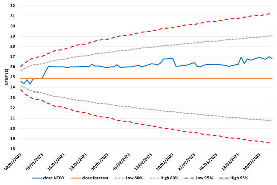
Figure 11.
NTGY stock closing prices from 2 January 2023 to 24 March 2023. Closing values, forecasted closing values, and 80% and 95% confidence intervals of the forecasting of the exponential smoothing MNN model.
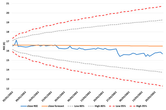
Figure 12.
REE stock closing prices from 2 January 2023 to 24 March 2023. Closing values, forecasted closing values, and 80% and 95% confidence intervals of the forecasting of the exponential smoothing MAN model.
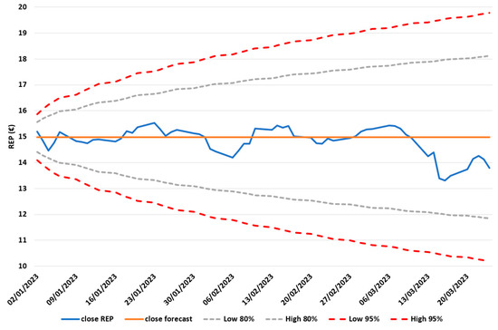
Figure 13.
REP stock closing prices from 2 January 2023 to 24 March 2023. Closing values, forecasted closing values, and 80% and 95% confidence intervals of the forecasting of the exponential smoothing ANN model.
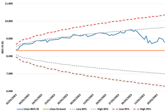
Figure 14.
IBEX35 index closing prices from 2 January 2023 to 24 March 2023. Closing values, forecasted closing values, and 80% and 95% confidence intervals of the forecasting of the exponential smoothing ANN model.
Table 4 shows the mean-squared error (MSE), root mean squared error (RMSE) [44], mean absolute error (MAE) [45], and percentage of points inside the 80% and 95% confidence interval of the models of the study when those models, calculated with historical prices from 2000 to 2022, are employed to forecast the prices from 2 January 2023 to 24 March 2023 and the forecasts obtained are compared with real values.
Table 4.
Mean-squared error (MSE), root mean squared error (RMSE), mean absolute error (MAE), and percentage of points inside the 80% confidence interval of the models (80% CI) of the models of the study. MAN: exponential smoothing with multiplicative errors and additive trend; MNN: exponential smoothing with multiplicative errors; and ANN: simple exponential smoothing with additive errors. ENG: ENAGÁS, ELE: ENDESA, IBE: IBERDROLA, NTGY: NATURGY, REE: Red Eléctrica Corporación, REP: REPSOL.
MSE is a widely used metric for evaluating the performance of predictive models in stock market forecasting. MSE is a measure of the average squared difference between the predicted and actual values and can provide insight into how well a forecasting model is able to predict stock prices. There are some examples in the existing literature that have utilized MSE in the assessment of stock market forecasting models [46,47].
RMSE is a popular metric used to evaluate the performance of predictive models in stock market forecasting. RMSE is similar to MSE, but it takes the square root of the average squared difference between predicted and actual values. It is commonly used to evaluate the accuracy of a model’s predictions, especially when there are outliers in the data. One reason why RMSE is useful in the presence of outliers is that it is less sensitive to extreme values than other metrics like mean absolute error (MAE). MAE gives equal weight to all errors, while RMSE squares each error, which amplifies the impact of larger errors. This means that RMSE is more influenced by larger errors but less influenced by outliers. One reason why RMSE is useful in the presence of outliers is that it penalizes large errors more heavily than small errors. This is because it squares the errors before taking the mean, so larger errors have a larger impact on the final score. As a result, the RMSE can be more useful in situations where it is important to identify and prioritize larger errors. One study that supports the use of RMSE in the presence of outliers [48] compared the performance of several regression metrics in the presence of outliers. It was found that RMSE performed better than other metrics like MAE and mean absolute percentage error (MAPE) in detecting the presence of outliers and was more accurate in predicting the true values of the response variable. Another study [49] found that RMSE was more robust to outliers than other metrics like mean absolute deviation (MAD) and was less likely to be influenced by the presence of a few large outliers. Please also note that many studies make use of RMSE in the assessment of stock market forecasting models [50,51].
MAE is another commonly used metric for evaluating the performance of predictive models in stock market forecasting. MAE measures the average absolute difference between predicted and actual values, and it is generally more interpretable than MSE or RMSE as it is in the same unit as the original data. The use of MAE is very common in the assessment of stock market forecasting models [52,53].
According to the results presented in Table 4, it can be said that the model with the lowest MSE value is exponential smoothing with multiplicative errors (MNN), which forecasts the closing stock price of IBERDROLA, followed by the model of the kind exponential smoothing with multiplicative errors and additive trend (MAN), which forecast stock close values of Red Eléctrica Corporación. The third model with the lowest MSE value is simple exponential smoothing with additive errors (ANN), which forecast the closure stock prices values of REPSOL. The same order applies to RMSE, as it is the root squared value of MSE, while in the case of MAE, the three models with the lowest values are again the MNN model that forecasts the closure stock prices of IBERDROLA, followed by REPSOL, which is an ANN model. The third model with the lowest values is the MAN model of Red Eléctrica Corporación. It is also noticeable that 100% of the real values forecasted by the models of ENDESA, IBERDROLA, NATURGY, Red Eléctrica Corporación, and REPSOL are inside the 80% confidence interval forecast for their respective models, while in the case of ENAGÁS, 96.72% of the daily closure values are inside this interval. In the case of the IBEX35 index, the figure is 93.95%. Finally, it is also remarkable that in all cases, all the real values of the forecasting period under study are inside the 95% CI of the models trained for all the time series.
The results presented in the previous paragraph allow us to say that none of the three kinds of models proposed with the best fits outperforms the others in all the cases, rather that it depends on the time series under study and also that the 80% confidence interval seems to be enough of a limit for the possible differences among real values and forecasts three months in advance.
4. Discussion
The results obtained in the present research confirm that time series analysis is a powerful tool for analyzing and forecasting stock prices in financial markets. Time series models can capture the patterns and trends in historical stock price data and use them to make predictions about future prices. From the authors’ point of view, there are several reasons why time series analysis is a valuable technique for stock market forecasting.
First, stock prices are influenced by trends and patterns that are related to time. These patterns can be weekly, monthly, or seasonal, and they can have a significant impact on stock prices. Time series models can capture these patterns and use them to make accurate predictions about future prices.
Second, time series models can help identify the underlying factors that drive stock price movements [54]. By analyzing historical data, time series models can identify the key variables that affect stock prices and use them to make predictions about future prices. This can be particularly useful for investors who want to understand the factors that are driving the market and make informed investment decisions.
Third, time series models can be used to estimate the volatility of stock prices [55]. Volatility is an important factor in investment decision-making, as it can indicate the level of risk associated with a particular investment. Time series models can be used to estimate volatility and help investors make informed decisions about the level of risk they are willing to take on. Please also note that even in a market condition like the one of 2023, the models proposed can provide a confidence interval in which most of the closing stock prices will be in the three following months. The authors want to point out that these results should be interpreted with caution.
We would like to remark that time series models can be used to analyze and predict the behavior of individual stocks or indexes, as has been done in the present research. By analyzing historical data, time series models can identify the trends and patterns that are unique to specific stocks or markets and use them to make accurate predictions about future prices. Overall, the interest in using time series methodologies for stock market forecasting is clear, given their ability to capture patterns, identify factors, estimate volatility, and analyze individual stocks or markets. By leveraging the power of time series analysis, investors can make more informed investment decisions and manage risk in the stock market better [56].
In the case of the forecasting methodology employed in the present research, exponential smoothing is a widely used method for forecasting stock prices in financial markets. The results obtained in the present research confirmed that exponential smoothing is a simple yet effective method for capturing trends and patterns in stock price data. The use of exponential smoothing has allowed us to model and forecast various aspects of stock prices, like level, trend, and seasonality. By modeling these different components, exponential smoothing can provide more accurate and detailed predictions of future stock prices.
According to the results obtained, it can be said that exponential smoothing can be easily adapted to handle different types of data and different levels of volatility. This makes it a flexible and robust method for forecasting stock prices in a variety of market conditions. Overall, the interest in using exponential smoothing methodologies for stock market forecasting is clear, given their simplicity, effectiveness, flexibility, and integration with other models. By leveraging the power of exponential smoothing, investors can make more accurate predictions of future stock prices and better manage risk in the stock market.
As has already been explained in this work, time series forecasting models like the one presented in this research are mathematical techniques that can analyze past data to make predictions about future values of a particular variable based on patterns and trends observed in historical data. From the point of view of the authors, these models can be used by investors and managers to make informed decisions regarding future investments or business strategies.
One way in which time series forecasting models can support investors is, like the work presented in this paper, by predicting future market trends, such as stock prices, exchange rates, or commodity prices. By analyzing historical data and identifying patterns and trends, these models can help investors make informed decisions about when to buy or sell assets and how much to invest in particular markets or industries.
Similarly, time series forecasting models can also be used by managers to predict future demand for products or services and to develop effective production and supply chain strategies accordingly. By analyzing past sales data and identifying trends and patterns, managers can make informed decisions about production schedules, inventory levels, and pricing strategies, which can ultimately help them to optimize their business operations and maximize profitability. Overall, time series forecasting models provide investors and managers with valuable insights into future trends and patterns, enabling them to make more informed decisions and stay ahead of the competition in today’s fast-paced business environment.
The fact that different models among the family of exponential smoothing have obtained the best performance for different time series highlights the complexity of the problem under study and the need for further research into this problem. One key consideration when using exponential smoothing is whether to model the errors as additive or multiplicative. In the case of the present research, both have shown the best performance for some of the stocks under study. The choice between these two approaches depends on the nature of the data being forecasted. In exponential smoothing with additive errors, the forecast error is assumed to be independent of the level of the time series. This means that it is assumed to be constant across time periods, regardless of the magnitude of the forecast. In contrast, exponential smoothing with multiplicative errors assumes that the forecast error is proportional to the level of the time series. This means that the magnitude of the forecast error increases or decreases as the level of the time series does the same. Multiplicative errors are appropriate when the size of the error is likely to be proportional to the level of the time series. As has already been said before, both models have proved the highest performance for different time series.
In the case of the forecasting model of ENG, the best performance was achieved by exponential smoothing with multiplicative errors and additive trends. The additive trend in exponential smoothing refers to a type of trend pattern in time series data that exhibits a linear increase or decrease over time with a constant amount. In other words, the amount of change in the trend is constant over time and can be expressed as a fixed value, which is added or subtracted from the level of the time series at each time period. The additive trend is modeled in exponential smoothing by adding a trend component to the basic exponential smoothing model. The trend component is then updated over time based on the observed data and the smoothing parameters. One of the advantages of using exponential smoothing with additive trends is that it is relatively simple and easy to interpret, as the trend component is expressed as a fixed value that can be easily visualized and understood. It also works well for time series data where the trend is relatively stable, and the magnitude of the change in the trend is consistent over time.
From the authors’ point of view, it would be of interest to introduce machine learning methodologies [57,58,59] in future research and compare the results obtained in this research with those that could be achieved by making use of these novel methodologies. It must also be taken into account that previous research [60,61] has found that machine learning models outperformed traditional statistical models in predicting stock prices, highlighting the potential of these techniques in stock market forecasting. Therefore, obtaining such good results by means of these methodologies in similar problems convinces the authors of this article to use them in future research.
Author Contributions
Conceptualization, I.B.T. and F.S.L.; data curation, I.B.T. and F.S.L.; formal analysis, I.B.T. and F.S.L.; methodology, F.S.L. and I.B.T.; project administration, F.S.L.; resources, F.S.L.; software, I.B.T. and F.S.L.; validation, F.S.L.; visualization, F.S.L.; writing—original draft, I.B.T.; writing—review and editing, I.B.T. and F.S.L. All authors have read and agreed to the published version of the manuscript.
Funding
This research was funded by Proyecto Plan Regional by Fundación para la Investigación Científica y Técnica (FICYT), Government of the Principality of Asturias, Spain, grant number SV-PA-21-AYUD/2021/51301 and Plan Nacional by Ministerio de Ciencia, Innovación y Universidades, Spain, grant number MCIU-22-PID2021-127331NB-I00.
Data Availability Statement
The data presented in this study is available on request to the corresponding author.
Acknowledgments
The authors would like to thank Anthony Ashworth for his revision of the English grammar and spelling in the manuscript.
Conflicts of Interest
The authors declare no conflict of interest.
References
- Chomać-Pierzecka, E.; Sobczak, A.; Urbańczyk, E. RES Market Development and Public Awareness of the Economic and Environmental Dimension of the Energy Transformation in Poland and Lithuania. Energies 2022, 15, 5461. [Google Scholar] [CrossRef]
- European Commission. Communication from the Commission to the European Parliament, the Council, the European Economic and Social Committee and the Committee of the Regions. The European Green Deal. Brussels, COM (2019) 640 Final. 11 December 2019. Available online: https://www.elni.org/fileadmin/elni/dokumente/Green_Deal-Sustainable_Products_Policy_2019-12-18_engl_fin.pdf (accessed on 29 April 2022).
- United Nations. Transforming Our World: The 2030 Agenda for Sustainable Development. A/RES/70/1. 2015. Available online: https://sustainabledevelopment.un.org/content/documents/21252030%20Agenda%20for%20Sustainable%20Development%20web.pdf (accessed on 29 April 2022).
- Siksnelyte-Butkiene, I.; Karpavicius, T.; Streimikiene, D.; Balezentis, T. The Achievements of Climate Change and Energy Policy in the European Union. Energies 2022, 15, 5128. [Google Scholar] [CrossRef]
- Steblyakova, L.P.; Vechkinzova, E.; Khussainova, Z.; Zhartay, Z.; Gordeyeva, Y. Green Energy: New Opportunities or Challenges to Energy Security for the Common Electricity Market of the Eurasian Economic Union Countries. Energies 2022, 15, 5091. [Google Scholar] [CrossRef]
- Available online: https://www.worldbank.org/en/news/press-release/2022/09/15/risk-of-global-recession-in-2023-rises-amid-simultaneous-rate-hikes (accessed on 3 November 2022).
- Iglesias-García, C.; Sáiz, P.A.; Burón, P.; Sánchez-Lasheras, F.; Jiménez-Treviño, L.; Fernández-Artamendi, S.; Al-Halabí, S.; Corcoran, P.; García-Portilla, M.P.; Bobes, J. Suicide, unemployment, and economic recession in Spain. In Revista de Psiquiatría y Salud Mental (English Edition); Elsevier: Amsterdam, The Netherlands, 2017; Volume 10, pp. 70–77. [Google Scholar] [CrossRef]
- Iglesias-García, C.; Sáiz, P.; García-Portilla, M.; Bousoño, M.; Jiménez-Trevino, L.; Sánchez-Lasheras, F.; Bobes, J. Effects of the economic crisis on demand due to mental disorders in Asturias: Data from the Asturias Cumulative Psychiatric Case Register (2000–2010). Actas Españolas Psiquiatr. 2014, 42, 108–115. [Google Scholar]
- García-Iglesias, J.M.; Rodríguez-San Julián, E. The Spanish financial crisis: A general view and a comparison with the Japanese experience. J. Bank. Regul. 2012, 13, 20–34. [Google Scholar]
- Sandoval, A.; Uribe, C.A.; Ortiz, A. Analysis of the factors that determine the price of energy in Colombia. Energy Sources Part B Econ. Plan. Policy 2018, 13, 362–369. [Google Scholar]
- Leal, V.B.; Aragão, J.A. The Impact of Geopolitics on Energy Prices: A Literature Review. J. Bus. Econ. 2020, 11, 212–223. [Google Scholar]
- Núñez, F.; Arcos-Vargas, A.; Villa, G. Efficiency benchmarking and remuneration of Spanish electricity distribution companies. In Utilities Policy; Elsevier: Amsterdam, The Netherlands, 2020; Volume 67, p. 101127. [Google Scholar] [CrossRef]
- Peñate-Valentín, M.C.; del Carmen Sánchez-Carreira, M.; Pereira, Á. The promotion of innovative service business models through public procurement. An analysis of Energy Service Companies in Spain. In Sustainable Production and Consumption; Elsevier: Amsterdam, The Netherlands, 2021; Volume 27, pp. 1857–1868. [Google Scholar] [CrossRef]
- Perez-Sindin, X.S.; Lee, J.; Nielsen, T. Exploring the spatial characteristics of energy injustice: A comparison of the power generation landscapes in Spain, Denmark, and South Korea. In Energy Research & Social Science; Elsevier: Amsterdam, The Netherlands, 2022; Volume 91, p. 102682. [Google Scholar] [CrossRef]
- Market Capitalization of Listed Domestic Companies. 2020. Available online: https://data.worldbank.org/indicator/CM.MKT.LCAP.CD (accessed on 10 January 2022).
- Fama, E. Efficient capital markets: A review of the theory. J. Financ. 1970, 25, 383–417. [Google Scholar] [CrossRef]
- Shmilovici, A.; Alon-Brimer, Y.; Hauser, S. Using a Stochastic Complexity Measure to Check the Efficient Market Hypothesis. Comput. Econ. 2003, 22, 273–284. [Google Scholar] [CrossRef]
- Borovkova, S.; Tsiamas, I. An ensemble of LSTM neural networks for high-frequency stock market classification. J. Forecast. 2019, 38, 600–619. [Google Scholar] [CrossRef]
- de Bondt, W.F.M.; Thaler, R. Does the Stock Market Overreact? J. Financ. 1985, 40, 793–805. [Google Scholar] [CrossRef]
- Caporale, G.M.; Gil-Alana, L.; Plastun, A. Short-Term Price Overreactions: Identification, Testing, Exploitation. Comput. Econ. 2018, 51, 913–940. [Google Scholar] [CrossRef]
- Muthusamy, S.K.; Kannan, R. Market Efficiency or Lack Thereof: A Critique and Rethinking on Corporate Governance. 2019. Available online: https://ssrn.com/abstract=2592843 (accessed on 10 November 2019).
- Todorov, I.B.; Sánchez Lasheras, F. Forecasting Applied to the Electricity, Energy, Gas and Oil Industries: A Systematic Review. Mathematics 2022, 10, 3930. [Google Scholar] [CrossRef]
- Box, G.E.; Jenkins, G.M.; Reinsel, G.C. Time Series Analysis: Forecasting and Control; John Wiley & Sons: Hoboken, NJ, USA, 2015. [Google Scholar]
- Cheng, L.; Shadabfar, M.; Sioofy Khoojine, A. A State-of-the-Art Review of Probabilistic Portfolio Management for Future Stock Markets. Mathematics 2023, 11, 1148. [Google Scholar] [CrossRef]
- Ayala, J.; García-Torres, M.; Noguera, J.L.V. Technical analysis strategy optimization using a machine learning approach in stock market indices. Knowl. Based Syst. 2021, 225, 107119. [Google Scholar] [CrossRef]
- Lohrmann, C.; Luukka, P.; Jablonska-Sabuka, M.; Kauranne, T. A combination of fuzzy similarity measures and fuzzy entropy measures for supervised feature selection. Expert Syst. Appl. 2018, 110, 216–236. [Google Scholar] [CrossRef]
- Krzemień, A.; Riesgo Fernández, P.; Suárez Sánchez, A.; Sánchez Lasheras, F. Forecasting European thermal coal spot prices. In Journal of Sustainable Mining; Elsevier: Amsterdam, The Netherlands, 2015; Volume 14, pp. 203–210. [Google Scholar] [CrossRef]
- Montgomery, D.C.; Jennings, C.L.; Kulahci, M. Time Series Analysis and Forecasting by Example, 4th ed.; John Wiley & Sons: Hoboken, NJ, USA, 2015. [Google Scholar]
- Chatfield, C. The Analysis of Time Series: An Introduction, 6th ed.; Chapman and Hall/CRC: Boca Raton, FL, USA, 2004. [Google Scholar]
- Dhyani, B.; Kumar, M.; Verma, P.; Jain, A. Stock Market Forecasting Technique using Arima Model. Int. J. Recent Technol. Eng. 2020, 8, 2694–2697. [Google Scholar] [CrossRef]
- Rubio, L.; Gutiérrez Rodríguez, A.J.; Forero, M.G. EBITDA Index Prediction Using Exponential Smoothing and ARIMA Model. Mathematics 2021, 9, 2538. [Google Scholar] [CrossRef]
- Schöneburg, E. Stock price prediction using neural networks: A project report. Neurocomputing 1990, 2, 17–27. [Google Scholar] [CrossRef]
- Wu, J.; Gyourko, J.; Deng, Y. Evaluating conditions in major Chinese housing markets. Reg. Sci. Urban Econ. 2012, 42, 531–543. [Google Scholar] [CrossRef]
- Chang, Y.; Wong, J.F. Oil price fluctuations and Singapore economy. Energ. Policy 2003, 31, 1151–1165. [Google Scholar] [CrossRef]
- Andrews, S.; Kwek, K.T.; Cho, C.W. Capturing long-tailed black swan risk in east asian currencies. In Proceedings of the 12th International Convention of the East Asian Economic Association, Seoul, Republic of Korea, 2–3 October 2010. [Google Scholar]
- Mamprin, C.; Rodrigues, L.H.; Ferreira, P.R. Forecasting with dynamic regression models: An application to the Brazilian inflation. Int. J. Forecast. 2020, 36, 1296–1311. [Google Scholar]
- Brewer, M.J.; Butler, A.; Cooksley, S.L. The relative performance of AIC, AICC and BIC in the presence of unobserved heterogeneity. In Methods in Ecology and Evolution; Freckleton, R., Ed.; Wiley: Hoboken, NJ, USA, 2016; Volume 7, pp. 679–692. [Google Scholar] [CrossRef]
- Pankratz, A.; Crainiceanu, C. Forecasting stock prices using exponential smoothing models. J. Forecast. 2018, 37, 441–454. [Google Scholar] [CrossRef]
- Hu, J.; He, K.; Zhu, J. Forecasting China’s economic growth by an ETS(A,M) model with external variables. J. Forecast. 2017, 36, 770–780. [Google Scholar] [CrossRef]
- Liu, Y.; Zhang, Y.; Zhao, Y. Forecasting stock prices using exponential smoothing with multiplicative errors. J. Forecast. 2019, 38, 185–200. [Google Scholar] [CrossRef]
- Peng, Z.; Lei, L.; Liu, Z.; Sun, J.; Ding, A.; Ban, J.; Chen, D.; Kou, X.; Chu, K. The impact of multi-species surface chemical observation assimilation on air quality forecasts in China. Atmos. Chem. Phys. 2018, 18, 17387–17404. [Google Scholar] [CrossRef]
- Zhang, X.; Wang, Y.; Liu, X.; Li, Y. Machine learning in stock price trend forecasting. J. Risk Financ. Manag. 2019, 12, 168. [Google Scholar]
- Chatterjee, A.; Islam, R.; Al-Sumaiti, A. Forecasting electricity demand in India: A simple exponential smoothing with additive errors model. J. Energy Storage 2019, 24, 100782. [Google Scholar] [CrossRef]
- Lee, M.-H.; Moon, H.-J. Nonintrusive Load Monitoring Using Recurrent Neural Networks with Occupants Location Information in Residential Buildings. Energies 2023, 16, 3688. [Google Scholar] [CrossRef]
- Willmott, C.J.; Matsuura, K. Advantages of the mean absolute error (MAE) over the root mean square error (RMSE) in assessing average model performance. Clim. Res. 2005, 30, 79–82. [Google Scholar] [CrossRef]
- Kumar, S.; Sharma, S. Predicting stock prices using technical analysis and machine learning algorithms. J. King Saud Univ.-Comput. Inf. Sci. 2021, 33, 67–76. [Google Scholar]
- Salim, R.A.; Srinivasan, D. Forecasting stock prices using hybrid ARIMA and neural network models. In Proceedings of the International Conference on Information Technology and Electrical Engineering (ICITEE), Phuket, Thailand, 12–13 October 2017; pp. 557–561. [Google Scholar]
- Greco, L.; Luta, G.; Krzywinski, M. Analyzing outliers: Robust methods to the rescue. Nat. Methods 2019, 16, 275–276. [Google Scholar] [CrossRef]
- Huang, H.; Wang, Q. An empirical comparison of the robustness of two statistical metrics for model validation. Chemom. Intell. Lab. Syst. 2015, 146, 399–406. [Google Scholar] [CrossRef]
- Hamzah, N.; Umaru, A.; Hussaini, A.A. A Comparative Analysis of Machine Learning Techniques for Stock Price Prediction. J. Inf. Commun. Technol. Res. 2021, 13, 117–125. [Google Scholar]
- İşcan, M.F.; Çelik, E. Comparison of ARIMA and Artificial Neural Networks Models in Forecasting Stock Prices. J. Financ. Stud. Res. 2021, 2021, 51–64. [Google Scholar]
- Kumar, M.; Gupta, V.; Rani, R. Stock price prediction using machine learning algorithms. J. Bus. Res. 2020, 117, 960–971. [Google Scholar]
- Nawi, N.M.; Aziz, A.A.; Yahaya, N. Stock price prediction using regression analysis, naïve Bayes, and k-nearest neighbors. Int. J. Electr. Comput. Eng. (IJECE) 2019, 9, 1792–1802. [Google Scholar]
- Gencay, R. Forecasting stock market volatility using technical analysis and machine learning techniques. Appl. Math. Comput. 2010, 217, 402–410. [Google Scholar]
- Tseng, F.M.; Li, H.Y. A hybrid model for stock price prediction. Expert Syst. Appl. 2012, 39, 1114–1121. [Google Scholar]
- Ghysels, E.; Wright, J.H. Forecasting professional forecasters. J. Bus. Econ. Stat. 2019, 37, 563–573. [Google Scholar]
- Casteleiro-Roca, J.-L.; Jove, E.; Sánchez-Lasheras, F.; Méndez-Pérez, J.-A.; Calvo-Rolle, J.-L.; de Cos Juez, F.J. Power Cell SOC Modelling for Intelligent Virtual Sensor Implementation. In Journal of Sensors; Hindawi Limited: London, UK, 2017; Volume 2017, pp. 1–10. [Google Scholar] [CrossRef]
- Sánchez, A.B.; Ordóñez, C.; Lasheras, F.S.; de Cos Juez, F.J.; Roca-Pardiñas, J. Forecasting SO2 Pollution Incidents by means of Elman Artificial Neural Networks and ARIMA Models. In Abstract and Applied Analysis; Hindawi Limited: London, UK, 2013; Volume 2013, pp. 1–6. [Google Scholar] [CrossRef]
- Ahmed, A.T.; Ali, M.; Almomani, O.; Al-Shorman, A.; Al-Emran, M. A review of machine learning techniques in financial forecasting. J. Financ. Data Sci. 2021, 7, 14–27. [Google Scholar]
- Chakraborty, D.; Adhikari, A. Stock market prediction using machine learning algorithms. J. Big Data 2018, 5, 1–18. [Google Scholar]
- Smith, J.A.; Johnson, K.L. A comparison of machine learning and traditional statistical models for predicting stock prices. J. Financ. Econ. 2020, 15, 45–63. [Google Scholar]
Disclaimer/Publisher’s Note: The statements, opinions and data contained in all publications are solely those of the individual author(s) and contributor(s) and not of MDPI and/or the editor(s). MDPI and/or the editor(s) disclaim responsibility for any injury to people or property resulting from any ideas, methods, instructions or products referred to in the content. |
© 2023 by the authors. Licensee MDPI, Basel, Switzerland. This article is an open access article distributed under the terms and conditions of the Creative Commons Attribution (CC BY) license (https://creativecommons.org/licenses/by/4.0/).