Article

A Parametric Physics-Informed Deep Learning Method for Probabilistic Design of Thermal Protection Systems

1
School of Mathematics and Science, North China Electric Power University, Beijing 102206, China
2
China Academy of Launch Vehicle Technology, Beijing 100076, China
3
School of Energy Power and Mechanical Engineering, North China Electric Power University, Beijing 102206, China
*
Authors to whom correspondence should be addressed.
Energies 2023, 16(9), 3820; https://doi.org/10.3390/en16093820
Submission received: 5 March 2023 / Revised: 19 April 2023 / Accepted: 26 April 2023 / Published: 29 April 2023
(This article belongs to the Special Issue Digital Twin Technology in Energy and Environmental Sector)

Abstract

:
Precise and efficient calculations are necessary to accurately assess the effects of thermal protection system (TPS) uncertainties on aerospacecrafts. This paper presents a probabilistic design methodology for TPSs based on physics-informed neural networks (PINNs) with parametric uncertainty. A typical thermal coating system is used to investigate the impact of uncertainty on the thermal properties of insulation materials and to evaluate the resulting temperature distribution. A sensitivity analysis is conducted to identify the influence of the parameters on the thermal response. The results show that PINNs can produce quick and accurate predictions of the temperature of insulation materials. The accuracy of the PINN model is comparable to that of a response surface surrogate model. Still, the computational time required by the PINN model is only a fraction of the latter. Considering both computational efficiency and accuracy, the PINN model can be used as a high-precision surrogate model to guide the TPS design effectively.

1. Introduction

The safety of the aerospacecraft relies heavily on the thermal protection system (TPS). However, the design and application of TPSs are subject to various uncertainties, such as size deviations during thermal protection parts production, external aerodynamic heating load uncertainties during operation, and changes in material physical properties due to variations in the environment’s temperature or the material itself [1]. Redundant design based on limit deviation has been conventionally employed to address these uncertainties, leading to a heavy weight of the TPS and decreased system performance [2]. Therefore, developing a high-precision approach to TPS design that accounts for various uncertainties is a critical advancement in the field [3].
The concept of probabilization is widely utilized to quantify uncertainty in the design of TPSs. The utilization of the Monte Carlo method to analyze the uncertainty of heat conduction parameters was first proposed by Howell [4], which laid the foundation for the probabilistic design of uncertainty. Dec et al. [5] integrated Monte Carlo methods with trajectory calculations and aerodynamic heating predictions from material response calculations. They used a finite difference calculation tool to establish the relationship between the dimensional design margin and the failure probability of the TPS. However, this approach necessitates calling the system model multiple times for computation, resulting in significant computational costs and reduced computational efficiency. Alternatively, the original high-precision complicated model can be substituted with a surrogate model to enhance computational efficiency while preserving accuracy [6,7,8,9,10]. A surrogate model refers to an approximation model that describes the relationship between the input and output of a system. It enables obtaining the corresponding output quickly based on the input, without resorting to complex high-precision calculations. Surrogate models offer low computational costs, and their results closely resemble those of high-precision models. Common surrogate models include the response surface method, Kriging surrogate models (Gaussian processes), radial basis functions, polynomial chaos expansions (PCE), and neural networks, among others. Ravishankar et al. [11] studied the uncertainty characteristics of TPSs and predicted the failure probability of TPSs using the response surface method. Tao et al. [12] used Kriging surrogates to quantify the effects of slot geometry deviations and mainstream condition fluctuations on the aero-thermal performance of endwalls. Wang et al. [13] used polynomial chaos expansion to optimize the reliability design of TPSs based on evidence theory. Guo et al. [14] optimized the parameters of the metallic TPS using Bayesian neural networks and genetic algorithms. Sensitivity analysis demonstrated the impact of each design variable on the thermal and mechanical response.
Conventional probabilistic design methods often require a large amount of labeled data for training models to construct response surfaces for large-scale simulations. However, some data can be expensive or unavailable for calculation or measurement in practical engineering applications. Furthermore, the “black box” nature of surrogate models and their dependence on training data can result in a lack of generalization and, in some cases, failure [15,16]. In recent years, methods that combine neural networks with known physical information have been developed, enhancing the network’s capacity for learning [17,18,19,20,21,22]. Among these methods, the physics-informed neural network (PINN) [18] has attracted more attention due to its success in using neural networks to approximate the solution of partial differential equations straightforwardly. PINNs can be trained solely with known physical information without requiring additional training data, making it applicable in cases where little or no data are available.
Moreover, the physical information constraint enhances the model’s interpretability by making predictions consistent with the physical information and improving its generalization capacity. Another significant advantage of the PINN over traditional surrogate models is its ability to solve parametric problems [23,24]. Uncertain parameters are utilized as input parameters to produce corresponding prediction results for varying parameter values. This approach enables swift result prediction for many parameters without requiring Monte Carlo methods to repeat the computation procedure multiple times.
This paper applies physics-informed deep learning methods to the design process of TPSs, considering the impact of uncertainty factors on the system and building a probabilistic design process for TPSs. Specifically, in the surrogate modeling part of the probabilistic design process of TPSs, this paper uses the parameterized PINN method to consider the impact of uncertainty in material properties on TPSs. This method only uses known physical information to constrain the model and can quickly predict different parameters without additional labeled data. In addition, this article compares this method with traditional response surface methods in extrapolation ability and computational efficiency, demonstrating the effectiveness of this method and its potential for practical industrial applications.
The structure of this paper is as follows: In the second section, the probabilistic design process and method for TPSs are introduced, focusing on the basic principles of PINNs and parameterized PINN algorithms. In the third section, the feasibility of the PINN surrogate model is validated through deterministic modeling. Then, an uncertainty PINN surrogate model is constructed and applied to the design process of TPSs. Additionally, the PINN results are compared with those of traditional response surface methods, taking into account the model’s extrapolation and generalization capabilities. The fourth section provides a summary and outlook of this article.

2. Methods

This section discusses the methods associated with the uncertainty design process of TPSs, with a particular emphasis on the principles of PINNs.

2.1. Thermal Protection System

During the high-speed flight, the surface of the TPS faces a severe aerothermal environment, resulting in the top surface temperature being higher than the bottom surface temperature and heat transferring from the outside to the inside. The rate of heat transfer is influenced by time, the geometric shape of the insulation material, and the material properties of the insulation. Therefore, the objective of TPS design is to control the insulation material’s thickness and properties, among other factors, to ultimately regulate the bottom surface temperature so that it remains below the maximum temperature that the system can withstand [25]. This process involves dealing with uncertainties, which can be challenging. However, using PINN can help address these challenges by incorporating known physical information to achieve accurate predictions, even when data are limited.
The following partial differential equation [26] can be used to represent the heat transfer problem associated with TPS.
ρ ( u ) c ( u ) u ( x , t ) t = ( k ( u ) u ( x , t ) ) + f ( x , t ) , x Ω , t [ 0 , T ]
When the internal heat source f (x, t) is ignored, and all physical parameters remain constant, the equation can be simplified to
ρ c u t = k ( 2 u x 2 + 2 u y 2 + 2 u z 2 ) , x , y , z Ω , t [ 0 , T ]
where u represents the bottom surface temperature as a function of the four independent variables at the location specified by the time coordinate t and the spatial coordinates x, y, and z; k, ρ, and c are the three physical parameters of the insulation material, denoted as the thermal conductivity, density, and specific heat capacity of the material, respectively; Ω denotes the spatial domain; and T denotes the maximum value of time.
The boundary conditions can be expressed as
u ( x , y , z , t ) = u D
( k u x + k u y + k u z ) = q N
( k u x + k u y + k u z ) = h ( u w u f )
where Equation (3) represents the Dirichlet boundary condition and uD represents the known temperature on that boundary; Equation (4) represents the Neumann boundary condition and qN represents the heat flux on that boundary; Equation (5) is the Robin boundary condition, h represents the heat exchange coefficient on that boundary, uw is the temperature on the boundary and uf is the temperature in the environment.
The initial condition can be expressed as
u ( x , y , z , 0 ) = u 0
where u0 is the initial temperature, the task for the TPS is to solve for these control equations, boundary conditions, and initial conditions to determine the temperature u of the response.

2.2. Uncertainty Design Process

The uncertainty design process for TPSs consists of two main parts, uncertainty analysis, and uncertainty optimization [27,28,29], shown in Figure 1. The uncertainty design process mainly includes the following steps:
(1)
Deterministic modeling: Firstly, traditional deterministic modeling is performed on the system. This involves mathematically abstracting and describing the TPS-related problems to simulate the real physical system, and analyzing each variable in the system as a deterministic constant.
(2)
Uncertainty input and uncertainty modeling: Based on this, the uncertain parameters that need to be considered are preliminarily determined according to the real environment and configuration requirements of the TPS, such as material properties, heat flux density, geometric shape, etc. These parameters are considered uncertain inputs, and each input’s probability distributions and range intervals are determined based on practical working experience and input into the model for uncertainty modeling.
(3)
Surrogate model: as the computational cost of high-precision models is significant, a surrogate model is constructed to approximate the original high-precision model.
(4)
Sampling and uncertainty propagation: Once the surrogate model is trained, it can quickly provide corresponding output results for a new input. Therefore, a large number of system response values can be obtained by drawing a large number of random samples for uncertain inputs and using surrogate models for fast calculations. This method is known as the Monte Carlo method. The Monte Carlo method can be used to propagate uncertainty in input variables through surrogate models.
(5)
Reliability analysis: based on this, the uncertainty of the system is analyzed, such as by quantitatively analyzing the distribution characteristics of system performance under uncertainty impact and calculating the reliability of the design scheme.
(6)
Correlation and sensitivity analysis and adjusting input uncertainty: The system is optimized based on the analysis results. If the reliability meets the requirements, the design process ends. Otherwise, the correlation and sensitivity analysis of the uncertain parameters in the previous inputs are performed. The parameters with low correlation can be removed from the uncertain inputs to reduce the complexity of surrogate model training. At the same time, the parameters with high sensitivity are adjusted and optimized, such as by reducing the uncertainty level of relevant parameters through process improvement methods.
(7)
Uncertainty optimization: finally, the adjusted model is trained again, and the above steps are repeated until the system meets the design requirements.
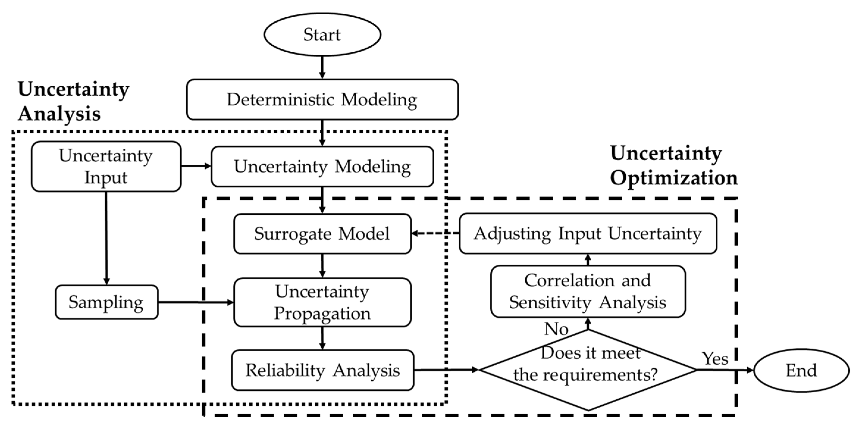
Figure 1. The uncertainty design process for thermal protection system (TPS).
Energies 16 03820 g001

2.3. Surrogate Model

High-precision numerical simulations are computationally expensive and can be replaced by a less costly surrogate model. A surrogate model is an approximate model that describes the input–output relationship of a system, which approximates the behavior of the actual system while ensuring computational efficiency. There are two types of surrogate models: physics-based and data-based. Physics-based surrogate models use known physical equations and parameters to describe the relationship between system inputs and outputs. Data-based surrogate models use existing experimental data and regression analysis to construct a functional relationship between inputs and outputs to replace the behavior of the actual system. Once trained, the model can quickly obtain the corresponding output results for new inputs without performing complex high-precision calculations. Since the evaluation cost of surrogate models is low, standard Monte Carlo methods can be used to consider uncertainty propagation in the model.
The commonly used surrogate model for a TPS is the response surface surrogate model. This section introduces the principles of the response surface, PINN, and parameterized PINN surrogate models.

2.3.1. Response Surface Methodology

The basic idea of response surface methodology is to use a polynomial expansion to approximate the relationship between input and output [30]. It has been mathematically proven that any function can be expressed by a polynomial. The response surface model generally uses only first- or second-order terms to fit the relationship, which can achieve satisfactory results while avoiding overfitting, despite the truncation error. The relationship obtained by the response surface model can be expressed as:
Y = X β + ε
where X and Y represent the input and output variables, respectively; β is the corresponding regression coefficient; and ε is the error between the fitted value and the true value. Generally, β can be determined by the least squares method, which means minimizing the error ε:
L = i = 1 n ε i 2 = ε ε = ( Y X β ) ( Y X β )
When the variance L is minimized, the response surface is obviously closest to the actual value. When the partial derivative of L with respect to β is 0, the minimum variance has a minimum value:
L β | β ^ = 2 X Y + 2 X X β ^ = 0
simplifying:
β ^ = ( X X ) 1 X Y
At this point, the expression fitted by the response surface surrogate model can be represented as:
Y = X β ^

2.3.2. Physics-Informed Neural Networks

The universal approximation theorem for neural networks is a theoretical result that shows that a neural network can approximate any continuous function to arbitrary precision [31]. This theorem forms the basis for the development of PINNs. Figure 2 provides a schematic representation of PINN. Since the output of a PINN is a continuously differentiable equation, each term in the differential equation can be calculated accurately using automatic differentiation [32]. PINN incorporates known physical information, such as partial differential equations, into the loss function of a neural network using automatic differentiation. This approach ensures that the neural network output is consistent with the known physical information. In general, parametric partial differential equations can be expressed as follows:
F ( x , t , u ( n ) ( x , t ) , λ ) = 0 , x Ω , t [ 0 , T ] u ( x , t 0 ) = g 0 ( x ) , x Ω u ( x , t ) = g Γ ( x ) , x Ω , t [ 0 , T ]
where x is a spatial coordinate vector and t is time; u(n)(x, t) denotes the n-th order derivative of the solution u(x, t) of the equation; λ denotes the parameter in the partial differential equation and F is the residual of the partial differential equation; g0(x) and gΓ(x) denote the initial and boundary conditions of the equation respectively, where the boundary conditions include three types of boundary conditions; Ω denotes a bounded region and ∂Ω is its corresponding boundary.
In a PINN, a fully connected neural network is used to approximate the solution to the equation u (x, t). An input layer, (K − 2) hidden layers, and an output layer make up a neural network with K layers. The neural network’s input parameters are the spatial and temporal coordinates (x, t), and its final layer’s output value is an approximation of the equation’s solution, u (x, t). Let the output vector of the i-th hidden layer be zi, then the neural network can be represented as:
z 0 = ( x , t ) z i = σ ( W i z i 1 + b i ) , i = 1 , , K 2 z K 1 = W K 1 z K 2 + b K 1
where z0 denotes the input layer of the neural network, zi(i = 1, …, K − 2) denotes the output vector of the i-th hidden layers, σ is the non-linear activation function, Wi and bi represent the weight matrix and bias vector of the i-th hidden layer respectively, which are parameters that need to be optimized during model training, and zK−1 is the approximate value of the solution u(x, t) of the equation.
A PINN essentially adds equations as physical restrictions to a neural network’s loss function, which is typically represented as:
L = α 1 L P D E + α 2 L I C + α 3 L B C
where the LPDE, LIC, and LBC correspond to the residuals of the control equations, initial conditions, and boundary conditions, respectively, where the partial differential operator can be easily obtained by automatic differentiation. α1, α2, and α3 are the weight coefficients of the corresponding loss terms, which can be adjusted according to the actual situation [33]. The PINN is trained to minimize the loss function by optimizing the parameters Wi and bi so that the solution learned by the neural network as closely as possible satisfies the known physical information. In general, Mean Square Error (MSE) is used to measure the loss of L, so the loss function can be written in the following form:
L = α 1 M S E P D E + α 2 M S E I C + α 3 M S E B C
where
M S E P D E = 1 N P D E i = 1 N P D E | F i 0 | 2 , M S E I C = 1 N I C i = 1 N I C | u ( x i , t 0 ) g 0 ( x i ) | 2 , M S E B C = 1 N B C i = 1 N B C | u ( x i , t i ) g Γ ( x i ) | 2

2.3.3. Parametric Physics-Informed Neural Networks

Parametric PINNs are a variation of the conventional PINN method that is better suited for solving parametric problems, such as uncertainty quantification and optimal design. In addition to the spatial and temporal coordinates (x, t) used in the standard PINN, the parametric PINN accepts the uncertainty parameter (λ) as an input to the neural network. This makes the input of the parametric PINN consist of spatiotemporal coordinates and the uncertainty parameter (x, t, λ). Figure 3 provides a comparison of the input layers of the two methods, with the rest of the principles being similar to those in Section 2.3.2.
In traditional methods, solving a problem for different parameters requires a new finite element analysis for each parameter, which is computationally expensive. On the other hand, the parametric PINN takes the parameters as input and can efficiently predict results for any given parameter value after training the model. Therefore, the parametric PINN significantly enhances computation efficiency by providing quick predictions for different parameters at a low computational cost.

2.4. Reliability Analysis

In TPS design, it is necessary to establish a reasonable range of reliability. If the system meets the reliability requirements, the design process is complete. However, if it fails to meet the requirements, the controllable parameters of the system must be optimized, and the reliability assessment must be repeated [34]. The reliability R of the TPS can be obtained directly from the statistical output as follows.
R = ( 1 N ( T lim T max ) N ) × 100 % = N ( T lim > T max ) N × 100 %
where Tlim is the limit temperature that the system can withstand and Tmax is the maximum bottom surface temperature of the system. N represents the total number of repetitions simulated using Monte Carlo sampling, and N(·) represents the number of times the corresponding situation occurs.

2.5. Correlation and Sensitivity Analysis

The probabilistic analysis of the temperature field of TPS has a significant advantage in providing the correlation and sensitivity of the output parameters to the input parameters [35]. This feature is useful in guiding system parameter tuning and industry-standard design. The correlation coefficient determines the relationship between each uncertain input parameter and the output temperature. It is an indicator that measures the linear correlation between the input and output. The expression of the correlation coefficient is given by:
r i = j = 1 n ( x i j x ¯ i ) ( y j y ¯ ) j = 1 n ( x i j x ¯ i ) 2 j = 1 n ( y j y ¯ ) 2 , i = 1 , 2 , 3
where ri denotes the correlation coefficient between the i-th input variable and the output variable y, which can indicate the degree of correlation between them; xij is the j-th value of the i-th input variable; x ¯ i is the mean value of the i-th input variable; yj is the j-th value of the output variable; ȳ is the mean value of the output variable.
Based on the correlation, the degree of influence of each input variable’s variability on the system’s reliability can be measured by the sensitivity coefficient. The sensitivity coefficient pi can be derived based on the correlation coefficient ri as described above, and its specific expression is:
p i = | r i | i = 1 n | r i |

3. Results

This section analyzes the transient heat transfer problem for TPSs using the method and process proposed in Section 2. The TPS studied in this paper is a typical large-area coating TPS, and its structural diagram is shown in Figure 4. The size of the three-dimensional model along the horizontal direction is much larger than that along the vertical direction. There is no shape change along the horizontal direction, so the temperature change in this direction can be ignored. Therefore, this paper simplifies the three-dimensional model into a one-dimensional one, consistent with the processing procedure in the [36].
This paper considers the homemade coating material, whose physical parameters are shown in Table 1 and Table 2. The material space length is set to L = 4 mm and the time is T = 150 s. The top surface boundary is a Neumann boundary condition with heat fluxes density of Q = 10,000 W·m−2, while the bottom surface boundary is an adiabatic condition. The initial temperature is set to 25 °C. The following partial differential equation can control the simplified model heat transfer performance:
{ u t k ρ c 2 u x 2 = 0 u x | x = 0 = Q k u x | x = 0.004 = 0 u | t = 0 = 25
where x belongs to the range [0, 0.004], and t belongs to the range [0, 150]. The training speed and accuracy of the neural network are influenced by the range of the input and output [37], so feature scaling is necessary before feeding the training data into the network. For the input variables (x, t), since the boundaries for the time and space parameters are predefined, they can be scaled to the range [0, 1] using the maximum values of time and space:
x ^ = x L , t ^ = t T
There is no pre-defined range for the output u. We normalized the output based on actual experience, with U being set to 100 in this case:
u ^ = u U
At this point, the previous equation also needs to be correspondingly modified:
{ u ^ t ^ k ρ c T L 2 2 u ^ x ^ 2 = 0 u x | x = 0 = L U Q k u x | x = 1 = 0 u | t = 0 = 25 U
where x belongs to the range [0, 1], and t belongs to the range [0, 1]. All subsequent examples in this paper will be discussed based on this equation.
Training of the PINN neural network does not require high-fidelity datasets, but to approximate the solution of partial differential equations, it needs to sample points at the boundary, initial time, and globally, and use them for training. In this paper, 200 points are randomly selected at the boundary and initial time respectively. In addition, to cover the predefined spatiotemporal domain more uniformly, this paper uses Latin hypercube sampling to sample the global configuration points, with a sample size of 10,000. These data are treated as training data.
The PINN surrogate models built in the examples of this paper were implemented on the TensorFlow platform with the following default settings. A fully connected neural network with four hidden layers, each with a width of 64, was used. The hyperbolic tangent function (tanh) was used as the activation function to ensure the smoothness of high-order derivatives of the developed neural network. The weight coefficients α in the loss function of the examples in this paper are all set to 1. The Adam optimizer was used for training first with a total number of training steps set to 5000. The hyperparameters of the Adam optimizer were set to l = 10−3, β1 = 0.9, and β2 = 0.999. Then, the L-BFGS-B algorithm was used for fine-tuning the neural network to obtain higher accuracy. The training process of L-BFGS-B was based on automatic termination with an incremental tolerance. Meanwhile, the response surface surrogate model and finite element method (FEM) constructed in the examples of this paper are implemented using ANSYS Parametric Design Language (APDL). The response surface constructed in this paper uses a quadratic polynomial to fit the relationship. Moreover, Monte Carlo simulations with a sample size of N = 10,000 were used to estimate the mean, standard deviation, and reliability. All training was performed on an NVIDIA GeForce GTX 1650 graphics processing unit (GPU).
In this section, to begin with, for the deterministic problem where material properties are considered as deterministic constants, a deterministic PINN surrogate model is established and extensively compared with the results obtained from the FEM, to verify the feasibility and effectiveness of the PINN surrogate model in the design of the TPS. Subsequently, uncertainty issues are considered, where material properties are no longer constants, but random variables following a certain distribution. These random variables are regarded as uncertain factors, and their effects on the design of the TPS are analyzed. Finally, we demonstrate the advantages of the PINN surrogate model in terms of extrapolation prediction and computational efficiency.

3.1. Deterministic PINN Surrogate Model

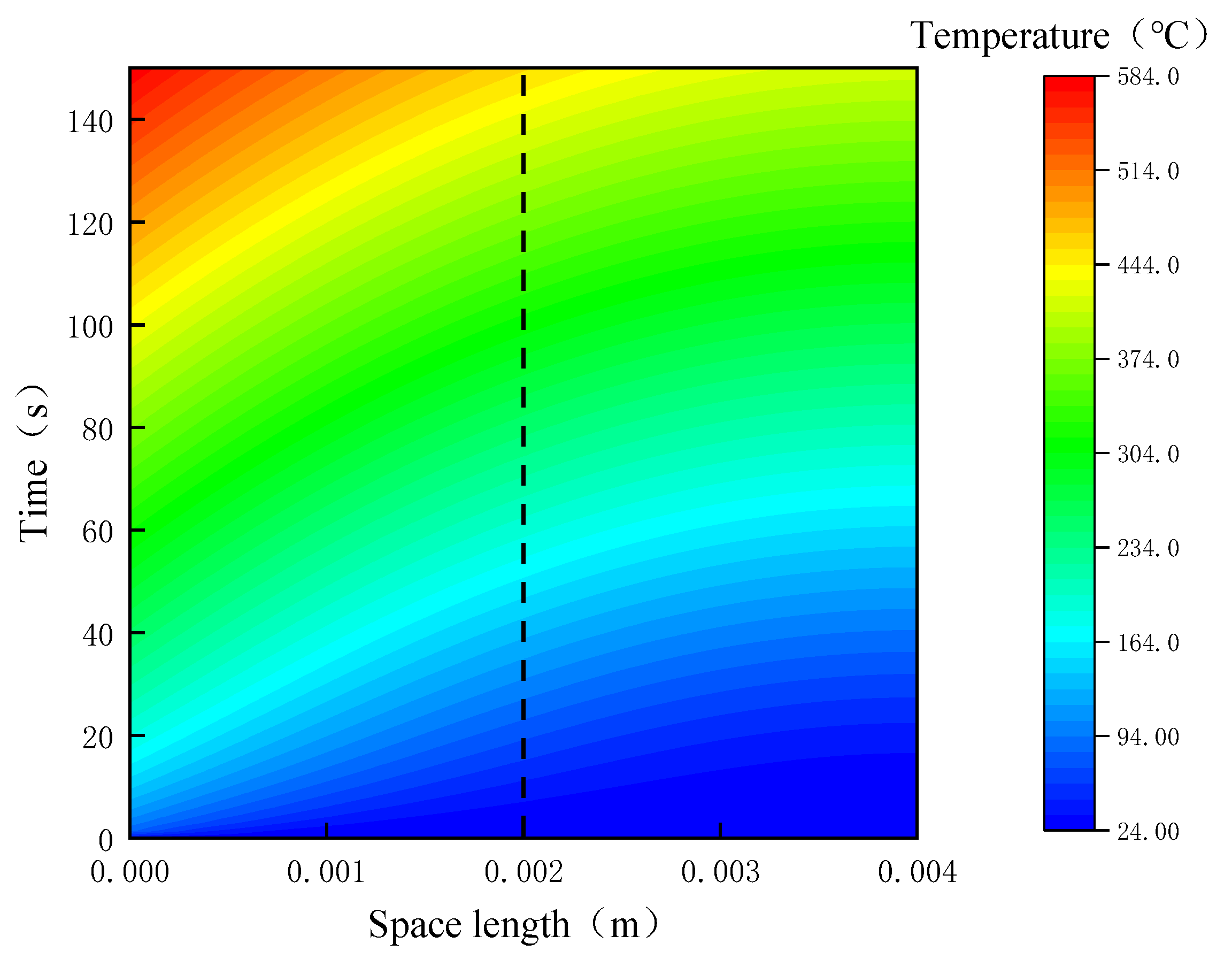
In this subsection, we present the development of a deterministic PINN heat transfer surrogate model for the TPS. The model assumes that the thermal conductivity, density, and specific heat capacity are constant values, and their respective values are specified in Table 1. Figure 5 illustrates the PINN surrogate model prediction results. The figure shows that the temperature of the material close to the top surface is relatively higher at the same time, and the variation in the material’s bottom surface temperature also rises over time. These trends are in good agreement with the actual physical behavior of the TPS.
A comparison is made between the prediction results of PINN and those of the FEM, and the results are presented in Figure 6 to further demonstrate the accuracy of the predictions. Figure 6 shows the temperature–time curves obtained by two methods at three locations, from top to bottom: the material’s top surface, the middle position, and the bottom surface (corresponding to x = 0 mm, 2 mm, and 4 mm, respectively). The dashed line in Figure 5 corresponds to the temperature–time curve at the middle position. The comparison reveals that there is a minimal disparity between the PINN prediction results and the corresponding numerical solutions, with a relative error of only 0.35%. These findings suggest that the PINN surrogate model can effectively simulate the temperature variation in insulation material with high accuracy.

3.2. Uncertain PINN Surrogate Model

This subsection modifies the assumption of fixed and constant values for material physical parameters by taking into account their variability and considering them as random parameters. This is motivated by the fact that the manufacturing process for the material can lead to uncertainties in the material’s properties, such as thermal conductivity, density, and specific heat capacity. To deal with these uncertainties, the parametric PINN method is used to achieve fast and accurate predictions of the temperature field. This approach is also applied to the uncertainty design process of TPS, where the effect of the uncertain parameters on the temperature distribution can be analyzed, and the design can be optimized accordingly.

3.2.1. Parametric PINN Surrogate Model

We consider the uncertainties associated with three mutually independent physical parameters: thermal conductivity, specific heat capacity, and density. Based on actual experimental measurements and engineering experience, each parameter is assumed to follow a truncated Gaussian distribution for stochastic modeling. The specific parameters of the distributions are provided in Table 2. The parameterized PINN is trained to obtain the temperature field on the bottom surface using these parameters along with spatial and time coordinates as the input for the neural network.
The predictive capabilities of three different methods were compared, namely, the FEM, response surface surrogate model, and parametric PINN surrogate model. Table 3 shows the corresponding bottom surface temperatures for these three methods’ results at t = 150 s under five different material property parameters, which are randomly selected. It was observed that both surrogate models could predict the temperature accurately. However, the response surface surrogate model provided results closer to the numerical results obtained from the FEM. In contrast, the parametric PINN surrogate model exhibited a deviation of approximately 3 °C from the accurate solution, with an average relative error of 0.76%. Nonetheless, this error level is considered acceptable and can be further reduced by optimizing the structure of the neural network or increasing the number of training iteration steps, etc. The loss function values during the training process of the parametric PINN surrogate model are illustrated in Figure 7. Logarithmic coordinates are employed to present the change in the loss function values more effectively. It can be observed from the graph that a marked decrease in the loss function values occurred when the L-BFGS-B optimizer was adopted after 5000 iterations of training.

3.2.2. Uncertainty Propagation

Upon completion of the training, the parametric PINN surrogate model is utilized to explore the uncertainty propagation of the parameters and their effect on the bottom surface temperature. To achieve this, 10,000 samples were extracted from the truncated Gaussian distribution of the three physical parameters, and the parametric PINN surrogate model quickly obtained their corresponding temperatures. Figure 8 displays the probability distribution characteristics of the extracted random array of thermal conductivity k, which approximately follows a normal distribution.
Figure 9 illustrates the properties of their corresponding bottom surface temperature probability distributions. By employing the same approach, the temperature results of the response surface surrogate model are depicted in Figure 10. A comparison of the statistical properties of the mean and standard deviation of the two predicted temperatures is presented in Table 4. The comparison reveals that the results of the parameterized PINN surrogate model are highly similar to those of the response surface surrogate model. Under the influence of parameter uncertainty, the bottom surface temperature of the TPS approximately conforms to a normal distribution. The mean temperature value predicted by the PINN is 414.94 °C, which is 3.43 °C higher than the response surface and concurs with the results of the previous samples. The difference in standard deviation between the two results is not statistically significant, indicating that the variations in predicted temperature results are relatively consistent.

3.2.3. Reliability Analysis

Here, the impact of uncertainties in material physical parameters on bottom surface temperature has been considered. Assuming a limit temperature of 450 °C for the system, 10,000 bottom surface temperatures have been obtained by sampling the parametric PINN surrogate model. Using these data, thermal reliability has been calculated to be R = 96.34%. However, this reliability value is low for practical engineering applications, indicating that the uncertainties in the parameters need to be reduced. Sensitivity analysis can be performed to determine the specific adjustments required. This analysis involves adjusting the input parameters that significantly influence the bottom surface temperature.

3.2.4. Correlation and Sensitivity Analysis

Table 5 presents the final correlation coefficients between the input parameters and the bottom surface temperature. The results indicate that both specific heat capacity and density exhibit a strong negative correlation with the bottom surface temperature, with correlation coefficients around −0.7. Specifically, specific heat capacity exhibits a stronger negative correlation than density, but the difference is insignificant. Furthermore, thermal conductivity exhibits only a 0.1 correlation with the temperature of the bottom surface. Hence, it can be inferred that there is no linear correlation between thermal conductivity and temperature, and it can be treated as a constant parameter for subsequent analysis in the design process. Figure 11, Figure 12 and Figure 13 illustrate the scatter plots of thermal conductivity, density, and specific heat capacity against temperature, respectively, providing a more visual representation of their correlation.
The sensitivity analysis based on the correlation coefficient was performed to assess the impact of physical parameters on temperature. Table 6 and Figure 14 present the results, indicating that the material’s density and specific heat capacity substantially influence the bottom surface temperature. In contrast, the impact of thermal conductivity is relatively insignificant. Therefore, further system optimization should focus on reducing the standard deviation of the material’s density and specific heat capacity to enhance the system’s thermal reliability.

3.3. PINN vs. Response Surface

3.3.1. Extrapolation Validation

In this subsection, the extrapolation performance of the parametric PINN surrogate model is examined, using Section 3.2 as an illustration. Specifically, the density is taken into consideration as a variable, with a range of [400, 700], while the thermal conductivity k and specific heat capacity c are set as constants with values corresponding to their respective means in Table 2. The PINN is then trained under these conditions. Subsequently, the trained model is used to predict temperatures in a varied range of densities of [400, 800], to assess the extrapolation capabilities of the PINN model. This result is compared with another PINN result in which the training range is directly in the global range, i.e., [400, 800]. Comparisons are made between the two results for the training range (i.e., [400, 700]) and the extrapolated range (i.e., [700, 800]). To observe the change in the temperature profile with density in this instance, the temperature at time t = 150 s and space x = 4 mm was selected. The results are presented in Figure 15.
Figure 15 reveals that the predictions obtained from both the training and extrapolation ranges are in agreement with the PINN prediction results derived from the global range training. An increase in density leads to a decrease in temperature. The extrapolation range exhibits a relatively high error of 0.48% compared to the average relative error of 0.19% for the training range. Nonetheless, this error remains within acceptable limits, which indicates the strong extrapolation capabilities of PINN. This can be attributed to PINN’s training to utilize governing equations, initial and boundary conditions, and other known physical information which constrains the model. Consequently, its interpretability, extrapolation, and generalization capabilities are enhanced. Furthermore, the computation range must be specified beforehand in numerical simulations, and only interpolation and calculations within that range are feasible, with poor extrapolation performance for values beyond that range.

3.3.2. Computational Efficiency

In this subsection, we compare the computational efficiency of the parametric PINN surrogate model and the response surface surrogate model in terms of their respective model-building times. Table 7 shows the results obtained using the same hardware. As discussed in Section 3.2.1, the accuracy of PINN is comparable to that of the response surface surrogate model. However, Table 7 reveals that PINN’s computation time is much shorter than that of the response surface model, being only 1/30 of the response surface’s computation time. The reason for this advantage of PINN over response surface methods is that response surface models require a fixed number of high-precision simulated data for training, while PINN does not require additional actual data for training the model. This leads to the longer computation time required for response surface training. Therefore, PINN offers a more computationally efficient approach than response surface methods.

4. Conclusions

This paper presents the PINN method’s application in the TPS design process. To demonstrate the feasibility of this method, a deterministic PINN surrogate model was first developed and trained using real engineering parameters. Subsequently, a parametric PINN surrogate model was constructed based on this to investigate the influence of uncertainty in three physical parameters, namely thermal conductivity, specific heat capacity, and density, on temperature. Finally, the performance of the PINN and the response surface surrogate models were compared. The following conclusions can be drawn:
  • In this study, the heat conduction equation of the TPS is used as an example, and the results show good agreement between the prediction results of the PINN surrogate model and those of numerical simulation, with a relative error of only 0.35 percent.
  • In terms of uncertainty propagation, the parametric PINN and response surface surrogate models effectively predict the results. However, parametric PINN is superior in extrapolation due to the constraint of physical information.
  • The PINN surrogate model is also more advantageous regarding computational efficiency, with a computation time of only 1/30 of that of the response surface surrogate model.
In conclusion, a PINN can be utilized as a high-precision surrogate model to produce an effective calculation for the design of a TPS. Since the PINN combines accuracy and computational efficiency, it also provides the potential for industrial application. Despite achieving high levels of accuracy in the above scenarios, the performance of PINN surrogate models can still be improved in further research extensions. In future studies, we plan to use the PINN surrogate model to solve more complex or higher-dimensional problems, making it more applicable to actual industrial design needs. For example, we can apply it to the uncertainty design of multi-layer thermal protection materials, or combine it with dimensionality reduction methods to solve actual high-dimensional problems.

Author Contributions

Conceptualization, K.Z. and R.Z.; methodology, R.Z.; software, N.X.; validation, L.W.; writing—original draft preparation, R.Z.; writing—review and editing, K.Z.; supervision, G.L.; project administration, K.Z.; funding acquisition, K.Z. All authors have read and agreed to the published version of the manuscript.

Funding

This research was funded by the National Natural Science Foundation of China, grant numbers 52276169 and 52076074, and the Fundamental Research Funds for the Central Universities (No. 2022JG006).

Data Availability Statement

No new data were created or analyzed in this study. Data sharing is not applicable to this article.

Conflicts of Interest

The authors declare no conflict of interest.

References

  1. Nakamura, T.; Fujii, K. Probabilistic transient thermal analysis of an atmospheric reentry vehicle structure. Aerosp. Sci. Technol. 2006, 10, 346–354. [Google Scholar] [CrossRef]
  2. Katsikas, C.; Castle, G.; Higgins, J. Ablation Handbook Entry Materials Data and Design; Air Force Materials Laboratory, Research and Technology Division, Air Force: Arlington, VA, USA, 1966. [Google Scholar]
  3. Dong, Y.; Wang, E.; You, Y.; Yin, C.; Wu, Z. Thermal Protection System and Thermal Management for Combined-Cycle Engine: Review and Prospects. Energies 2019, 12, 240. [Google Scholar] [CrossRef]
  4. Howell, J.R. Monte Carlo treatment of data uncertainties in thermal analysis. J. Spacecr. Rocket. 1973, 10, 411–414. [Google Scholar] [CrossRef]
  5. Dec, J.; Mitcheltree, R. Probabilistic design of a Mars Sample Return Earth entry vehicle thermal protection system. In Proceedings of the 40th AIAA Aerospace Sciences Meeting & Exhibit, Reno, NV, USA, 14–17 January 2002; p. 910. [Google Scholar]
  6. Woo, M.-A.; Moon, Y.-H.; Song, W.-J.; Kang, B.-S.; Kim, J. Acquisition of Dynamic Material Properties in the Electrohydraulic Forming Process Using Artificial Neural Network. Materials 2019, 12, 3544. [Google Scholar] [CrossRef] [PubMed]
  7. Cunha, B.Z.; Zine, A.-M.; Ichchou, M.; Droz, C.; Foulard, S. On Machine-Learning-Driven Surrogates for Sound Transmission Loss Simulations. Appl. Sci. 2022, 12, 10727. [Google Scholar] [CrossRef]
  8. Sun, Y.; Elhanashi, A.; Ma, H.; Chiarelli, M.R. Heat Conduction Plate Layout Optimization Using Physics-Driven Convolutional Neural Networks. Appl. Sci. 2022, 12, 10986. [Google Scholar] [CrossRef]
  9. Lyathakula, K.R.; Yuan, F.-G. A probabilistic fatigue life prediction for adhesively bonded joints via ANNs-based hybrid model. Int. J. Fatigue 2021, 151, 106352. [Google Scholar] [CrossRef]
  10. Alqahtani, A.; He, X.; Yan, B.; Hoteit, H. Uncertainty Analysis of CO2 Storage in Deep Saline Aquifers Using Machine Learning and Bayesian Optimization. Energies 2023, 16, 1684. [Google Scholar] [CrossRef]
  11. Ravishankar, B.; Haftka, R.; Sankar, B. Uncertainty analysis of integrated thermal protection system with rigid insulation bars. In Proceedings of the 52nd AIAA/ASME/ASCE/AHS/ASC Structures, Structural Dynamics and Materials Conference 19th AIAA/ASME/AHS Adaptive Structures Conference 13t, Denver, CO, USA, 4–7 April 2011; p. 1767. [Google Scholar]
  12. Tao, Z.; Guo, Z.; Song, L.; Li, J. Uncertainty quantification of aero-thermal performance of a blade endwall considering slot geometry deviation and mainstream fluctuation. J. Turbomach. 2021, 143, 111013. [Google Scholar] [CrossRef]
  13. Wang, C.; Matthies, H.G. Evidence theory-based reliability optimization design using polynomial chaos expansion. Comput. Methods Appl. Mech. Eng. 2018, 341, 640–657. [Google Scholar] [CrossRef]
  14. Guo, Q.; Wang, S.; Hui, W.; Li, Y.; Xie, Z. Thermo-mechanical optimization of metallic thermal protection system under aerodynamic heating. Struct. Multidiscip. Optim. 2020, 61, 819–836. [Google Scholar] [CrossRef]
  15. LeCun, Y.; Bengio, Y.; Hinton, G. Deep learning. Nature 2015, 521, 436–444. [Google Scholar] [CrossRef] [PubMed]
  16. Cai, S.; Wang, Z.; Wang, S.; Perdikaris, P.; Karniadakis, G.E. Physics-informed neural networks for heat transfer problems. J. Heat Transf. 2021, 143, 060801. [Google Scholar] [CrossRef]
  17. Sirignano, J.; Spiliopoulos, K. DGM: A deep learning algorithm for solving partial differential equations. J. Comput. Phys. 2018, 375, 1339–1364. [Google Scholar] [CrossRef]
  18. Raissi, M.; Perdikaris, P.; Karniadakis, G.E. Physics-informed neural networks: A deep learning framework for solving forward and inverse problems involving nonlinear partial differential equations. J. Comput. Phys. 2019, 378, 686–707. [Google Scholar] [CrossRef]
  19. Yu, B. The deep Ritz method: A deep learning-based numerical algorithm for solving variational problems. Commun. Math. Stat. 2018, 6, 1–12. [Google Scholar]
  20. Lu, L.; Jin, P.; Karniadakis, G.E. Deeponet: Learning nonlinear operators for identifying differential equations based on the universal approximation theorem of operators. arXiv 2019, arXiv:1910.03193. [Google Scholar]
  21. Li, Z.; Kovachki, N.; Azizzadenesheli, K.; Liu, B.; Bhattacharya, K.; Stuart, A.; Anandkumar, A. Fourier neural operator for parametric partial differential equations. arXiv 2020, arXiv:2010.08895. [Google Scholar]
  22. Chu, W.X.; Lien, Y.H.; Huang, K.R.; Wang, C.C. Energy saving of fans in air-cooled server via deep reinforcement learning algorithm. Energy Rep. 2021, 7, 3437–3448. [Google Scholar] [CrossRef]
  23. Sun, L.; Gao, H.; Pan, S.; Wang, J.-X. Surrogate modeling for fluid flows based on physics-constrained deep learning without simulation data. Comput. Methods Appl. Mech. Eng. 2020, 361, 112732. [Google Scholar] [CrossRef]
  24. Gao, H.; Sun, L.; Wang, J.-X. PhyGeoNet: Physics-informed geometry-adaptive convolutional neural networks for solving parameterized steady-state PDEs on irregular domain. J. Comput. Phys. 2021, 428, 110079. [Google Scholar] [CrossRef]
  25. Marley, C.D.; Driscoll, J.F. Modeling an active and passive thermal protection system for a hypersonic vehicle. In Proceedings of the 55th AIAA Aerospace Sciences Meeting, Grapevine, TX, USA, 9–13 January 2017; p. 0118. [Google Scholar]
  26. Holman, J.P. Heat Transfer; McGraw Hill Higher Education: New York, NY, USA, 2010. [Google Scholar]
  27. Wright, M.J. NASA Uncertainties Management in the TPS Design Process. In Proceedings of the 4TH AF/SNL/NASA Ablation Workshop, Albuquerque, NM, USA, 1–3 March 2011. [Google Scholar]
  28. Sun, J.; Zhang, G.; Vlahopoulos, N.; Hong, S.-B. Multi-disciplinary design optimization under uncertainty for thermal protection system applications. In Proceedings of the 11th AIAA/ISSMO Multidisciplinary Analysis and Optimization Conference, Portsmouth, VA, USA, 6–8 September 2006; p. 7002. [Google Scholar]
  29. Vlahopoulos, N.; He, J. Designing the Thermal Protection System of an Apollo Type Vehicle under Uncertainty; 0148-7191; SAE Technical Paper: Warrendale, PA, USA, 2009. [Google Scholar]
  30. Bezerra, M.A.; Santelli, R.E.; Oliveira, E.P.; Villar, L.S.; Escaleira, L.A. Response surface methodology (RSM) as a tool for optimization in analytical chemistry. Talanta 2008, 76, 965–977. [Google Scholar] [CrossRef] [PubMed]
  31. Hornik, K.; Stinchcombe, M.; White, H. Universal approximation of an unknown mapping and its derivatives using multilayer feedforward networks. Neural Netw. 1990, 3, 551–560. [Google Scholar] [CrossRef]
  32. Baydin, A.G.; Pearlmutter, B.A.; Radul, A.A.; Siskind, J.M. Automatic differentiation in machine learning: A survey. J. Marchine Learn. Res. 2018, 18, 1–43. [Google Scholar]
  33. Wang, S.; Teng, Y.; Perdikaris, P. Understanding and mitigating gradient flow pathologies in physics-informed neural networks. SIAM J. Sci. Comput. 2021, 43, A3055–A3081. [Google Scholar] [CrossRef]
  34. Paté-Cornell, M.-E.; Fischbeck, P.S. Risk management for the tiles of the space shuttle. Interfaces 1994, 24, 64–86. [Google Scholar] [CrossRef]
  35. Tortorelli, D.A.; Michaleris, P. Design sensitivity analysis: Overview and review. Inverse Probl. Eng. 1994, 1, 71–105. [Google Scholar] [CrossRef]
  36. Brune, A.J.; West, T.K.; Hosder, S. Uncertainty quantification of planetary entry technologies. Prog. Aeosp. Sci. 2019, 111, 17. [Google Scholar] [CrossRef]
  37. Ioffe, S.; Szegedy, C. Batch normalization: Accelerating deep network training by reducing internal covariate shift. In Proceedings of the International Conference on Machine Learning, Lille, France, 6–11 July 2015; pp. 448–456. [Google Scholar]
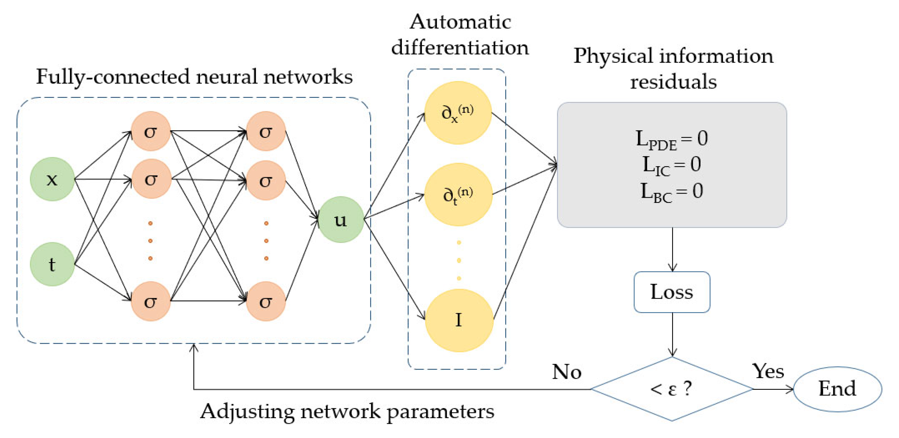
Figure 2. Schematic of a physics-informed neural network (PINN).
Energies 16 03820 g002
Figure 3. Comparison of the input layer of conventional PINN and parametric PINN.
Energies 16 03820 g003
Figure 4. Schematic diagram of homemade coating material TPS.
Energies 16 03820 g004
Figure 5. Prediction results of the PINN surrogate model in the entire spatiotemporal domain.
Energies 16 03820 g005
Figure 6. Comparison of prediction results between PINN surrogate model and FEM at three different locations. x = 0 mm, 2 mm, and 4 mm, respectively. The solid blue line represents the FEM results, while the dashed red line represents the PINN prediction results.
Energies 16 03820 g006
Figure 7. The training progresses of parametric PINN surrogate model.
Energies 16 03820 g007
Figure 8. Probability distribution of the values of thermal conductivity.
Energies 16 03820 g008
Figure 9. Probability distribution of the bottom surface temperature by parametric PINN surrogate model.
Energies 16 03820 g009
Figure 10. Probability distribution of the bottom surface temperature by the response surface surrogate model.
Energies 16 03820 g010
Figure 11. Scatter plot of thermal conductivity vs. temperature.
Energies 16 03820 g011
Figure 12. Scatter plot of density vs. temperature.
Energies 16 03820 g012
Figure 13. Scatter plot of specific heat capacity vs. temperature.
Energies 16 03820 g013
Figure 14. Correlation coefficient and sensitivity coefficient results.
Energies 16 03820 g014
Figure 15. Comparison of extrapolation results of PINN surrogate models.
Energies 16 03820 g015
Table 1. Parameter setting of material property parameters for deterministic modeling.
Input ParameterSymbolValueUnit
thermal conductivityk0.12W·m−1·K−1
densityρ560kg·m−3
specific heat capacityc1510J·kg−1·°C−1
Table 2. Parameter setting of material property parameters for uncertainty modeling.
Input ParameterSymbolUnitMeanStandard DeviationUpper BoundLower Bound
thermal conductivitykW·m−1·K−10.120.0030.130.10
densityρkg·m−356014602518
specific heat capacitycJ·kg−1·°C −115103816241396
Table 3. The temperature values of the bottom surface at t = 150 s with different parameters calculated by the three different methods.
Thermal
Conductivity
DensitySpecific Heat
Capacity
Finite Element MethodResponse Surface Surrogate ModelParametric PINN Surrogate Model
0.119370539.6451528.84421.728421.912424.996
0.116521558.4811513.49409.513409.433412.654
0.120067563.6181515.11406.717406.515409.758
0.122154584.5241546.61383.424383.177386.121
0.117357542.7461523.59419.727419.806422.894
Table 4. Comparison of the statistical properties of bottom surface temperature for two surrogate models.
MethodMeanStandard Deviation
parametric PINN414.9415.94
response surface411.5115.67
Table 5. The correlation coefficient between input and output.
MethodThermal ConductivityDensitySpecific Heat Capacity
parametric PINN0.101−0.697−0.709
response surface0.077−0.694−0.695
Table 6. Sensitivity coefficient between input and output.
Thermal ConductivityDensitySpecific Heat Capacity
temperature0.06720.47020.4626
Table 7. Comparison of the computational efficiency of parametric PINN and response surface surrogate models.
MethodTime
parametric PINN18.48 min
response surface597.24 min
Disclaimer/Publisher’s Note: The statements, opinions and data contained in all publications are solely those of the individual author(s) and contributor(s) and not of MDPI and/or the editor(s). MDPI and/or the editor(s) disclaim responsibility for any injury to people or property resulting from any ideas, methods, instructions or products referred to in the content.