Article

Generation of Synthetic CPTs with Access to Limited Geotechnical Data for Offshore Sites

1
UCD Centre for Mechanics, Dynamical Systems and Risk Laboratory, School of Mechanical and Materials Engineering, University College Dublin, D04 V1W8 Dublin, Ireland
2
Gavin & Doherty Geosolutions, D14 X627 Dublin, Ireland
3
School of Earth Sciences, Science Centre West, University College Dublin, D04 V1W8 Dublin, Ireland
4
SFI Research Centre in Applied Geosciences (iCRAG), O’Brien Centre for Science (East), University College Dublin, Belfield, D04 V1W8 Dublin, Ireland
5
Structural Dynamics and Assessment Laboratory, School of Civil Engineering, University College Dublin, D04 V1W8 Dublin, Ireland
*
Author to whom correspondence should be addressed.
Energies 2023, 16(9), 3817; https://doi.org/10.3390/en16093817
Submission received: 24 March 2023 / Revised: 19 April 2023 / Accepted: 20 April 2023 / Published: 28 April 2023

Abstract

:
The initial design phase for offshore wind farms does not require complete geotechnical mapping and individual cone penetration testing (CPT) for each expected turbine location. Instead, background information from open source studies and previous historic records for geology and seismic data are typically used at this early stage to develop a preliminary ground model. This study focuses specifically on the interpolation and extrapolation of cone penetration test (CPT) data. A detailed methodology is presented for the process of using a limited number of CPTs to characterise the geotechnical behavior of an offshore site using artificial neural networks. In the presented study, the optimised neural network achieved a predictive error of 0.067 . Accuracy is greatest at depths of less than 10 m . The pitfalls of using machine learning for geospatial interpolation are explained and discussed.

1. Introduction

The European Commission has set the ambitious goal of carbon neutrality by 2050 [1]. The objective of this strategy is to minimise the impact of the energy sector on climate change and ensure energy security, [2]. Under this recent strategy, it was decided that Europe’s offshore capacity would be increased from the then existing 12 G W to at least 60 G W by 2030 and to 300 G W by 2050, putting increased pressure over the offshore wind energy industry.
Ground condition characterization is a key step in any offshore wind farm (OWF) development project during the early phases to assess the project feasibility or during the later stages to support the ground modelling. Cone penetration testing (CPT) is generally the tool of choice for geotechnical site investigations offshore [3,4,5,6]. It can be used in a variety of soil conditions and it provides information about the mechanical properties of the soil, such as strength, stiffness and compressibility, as well as a repeatable index of the aggregate behaviour of the soil in the immediate area of the probe. CPT provides a lot of advantages for investigating soil properties. It is a fast and continuous soil profiling method, and it offers repeatable and reliable data [7].
Whilst a powerful sub-surface characterisation tool and economical over comparative SI techniques (e.g., boreholes), CPT still represents a sizeable commitment, both in terms of survey cost and time for any OWF development. Therefore, the focus of much research has been on optimising the use of gathered data, especially at early feasibility study stages of such engineering projects. Recent developments in the intelligent ground modelling and synthetic-CPT (Syn-CPT) generation are showing promise as a reliable method to fill the gaps during site characterization [3,8,9,10]. As the synthetic CPTs can be generated at any specific locations, reliably estimating ground conditions at an early stage helps with the planning of future developments, during which targeted ground investigations should be carried out [3,9].
Machine learning is increasingly being applied as a method in various fields to handle large and complex datasets. The advantages of machine learning include that it can extract multivariate, non-linear and non-stationary relationships by learning through data, provided that sufficient data are available [11,12]. Geotechnical data may exhibit non-stationary, multivariate feature dependency and non-linearity, rendering other methods, such as Kriging, unable to capture the breadth of the problem. In fact, Sauvin et al. [9], while not quantifying, acknowledged that uncertainty associated with the Kriging method applied to Syn-CPT is large and highly dependent on the distance between in situ test locations. Rauter and Tschuchnigg [13] used machine learning to classify soil types into its different categories of sand or clay. This study trained artificial neural networks (ANNs) on 1339 CPT profiles. Instead of obtaining geographical variation in the geotechnical properties, as has been achieved in the other studies, it [13] focuses on automatically identifying the soil type in each segment of the CPT profile using supervised learning. Rauter and Tschuchnigg [13] optimised their algorithm by routing the inputs through a random forest algorithm before feeding it into the NN, and concluded that this technique can be a cheaper alternative to expensive third-party solutions [14].
Sauvin et al. [9] compared ground models built using neural networks with industry standard geo-statistical approaches, into which 2D seismic data, borehole and CPT data were used to develop a quantitative ground model using two different approaches. The ANNs were reported to be superior in performance to the geo-statistical ground models. Carpentier et al. [10] followed a similar approach in applying supervised learning to obtain continuous geotechnical information for the initial study of a target offshore wind farm in western Holland. They trained CNNs on 2D ultra high resolution multi-channel seismic data coupled with CPT data. They trained their network on 1.5 million traces over the entire area of the test site, and reported good agreement between the predicted geotechnical properties in the testing dataset, especially in the upper 20 m of the sea-floor. Similarly, Vardy et al. [15] integrated geophysical parameters derived from seismic data, namely quality factors and acoustic impedance, to be used as input variables into an ANN. They highlighted the different sensibilities of geophysical and geotechnical parameters to soil behaviour variations, requiring further work to realistically quantify the interpretation error/confidence.
In this study, the generation of Syn-CPTs in situations with limited in situ data availability is examined. The main objective of this paper is to identify the techniques to generate the most accurate predictions whilst working with raw CPT data that present with significant variation in signals. To further the technical aspect of this challenge, the predictive parameters generated are analysed with regards to ANN performance and architecture for a specific case study. Based on the results of this study, the Syn-CPT generation with limited inputs is discussed regarding their implications for offshore wind farm site investigation.

2. Study Area and Data Sets

2.1. Cone Penetration Testing (CPT)

Understanding the physical significance of the various properties measured by the CPT allows us to determine which quantities would be crucial for predicting the geotechnical properties of a site. In a CPT, the cone unit (see Figure 1) is mounted at the end of a shaft made up of a series of rods, and is pushed into the ground at a constant rate. Continuous measurements are made of the resistance experienced by the cone and the surface of the sleeve. Cone tip resistance ( q c ) and sleeve friction ( f s ) are the two main measured parameters. Soil behaviour predictions can be improved with pore pressure measurements ( u 2 ). CPT can operate in soft soils as well as very stiff soils and in some cases, soft rock as well [7].
The terminology used in the Figure 1 and the definition of the extracted data from the CPT is given in Table 1. Typically, cone resistance ( q c ) values are observed to be higher in sands and lower in clays, and the friction ratio ( R e = f s / q c ) is low in sands and high in clays [7]. Usually, q c values are corrected from pore pressure ( u 2 ) effects and expressed as q t (Table 1). In soft clays and silt, pore pressures can be very large. The opposite is true if the soil is over-consolidated clay, dense silt or silty sand.

2.2. Site Description

The study area is in the northern Irish Sea, approximately 18 km offshore from the Dunany Point in Co. Louth at its most northerly point and Braymore Point in Co. Dublin at its most southerly (Figure 1B). This area extends within the the Western Irish MudBelt (WISMB), covering a large section of the northern Irish Sea [17,18,19,20]. This mud unit corresponds to recent sediment (Holocene age) that has blanketed the northern Irish Sea. Regarding the geological history of the area, the last glaciation and deglaciation episodes have been extensively studied [17,19,20,21] and proven to have had a major influence on sub-seabed conditions [17]. Coughlan et al. [17] proposed a stratigraphic model for the northern Irish Sea. Based on seismic and CPT data based on the correlation with the geological formations recognised from the BGS 89/15 borehole [22] and descriptions from Jackson et al. [19], the geology of the area can be generally described by the following succession from seafloor surface to top of the rockhead: marine mud, prodeltaic sands, heterogeneous coarse glaciomarine or glaciolacustrine sediments and glacial units consisting of cobbles in a matrix of stiff clay and recognised as a till formation. A more detailed description and information on variation can be found in Coughlan et al. [17] and Michel et al. [23]. Belderson [18] also observed the occurrence of shallow gas. The extent of the shallow gas has been mapped by Coughlan et al. [24].
In January 2022, an offshore survey (CE22 002 onboard the RV Celtic Explorer) was conducted to acquire new CPT data as part of the Sustainable Energy Authority of Ireland (SEAI) funded Informing and Mapping the Offshore Renewable Environment (I-MORE) project. The main objective of I-MORE was to improve the characterisation of sub-seabed sediment units by integrating legacy geophysical data to develop an updated geotechno-stratigraphic framework and classification for the Irish specific seabed conditions. During the survey, 24 locations were investigated using a Geomil Manta-200 CPT system (Figure 1C). within water depths ranging from 25 m to 58 m (Figure 1). The exact coordinates for each of the 24 locations have been recorded with ultra-short baseline (USBL) beacons fixed to the CPT device. The serial numbers are also the unique identifiers with which the data is stored.
The S. numbers that include ‘a’ are a repeated CPT at that location. The initial test was abandoned and the cone pulled out due to unsatisfactory results related to technical factors. For instance, S. No 5 and 5a have virtually the same location; however, the little difference between their coordinates comes from the relocation of the CPT unit to avoid the footprint of the initial test at that location.

3. Methodology

The current work develops an artificial neural network (ANN) for the spatial interpolation of CPT data. Machine learning is stochastic in nature, not deterministic. An ANN does not understand geophysics, and thus can not be constrained to abide by the laws of physics. For instance, it does not know that a negative corrected cone resistance ( q t ) is a non-physical attribute and does not exist in the real world. Simply put, AI does not recognise the relationship between cause and effect [25]. It only maps inputs onto outputs, but fails to generalise on unseen data. Therefore, the model developed first carries out data formatting, including smoothing to remove outliers and data points that give non-physical results. In the context of this study, the data were carefully averaged. Whilst the peaks themselves were removed, the effect of the peak in indicating a change in the soil morphology is registered by manually adjusting the data smoothing technique and its relevant parameters. Additionally, information on data normalisation and the architecture of the ANN used is mentioned. Finally, different hyperparameters used in the architecture are evaluated and compared to achieve the highest predictive accuracy on the testing dataset.

3.1. Inputs

The current model uses CPT data coordinates, depth and bathymetry as the inputs. The coordinates are defined in terms of the latitude and longitude and are expressed in decimal degrees (WGS84). The location of each of the sites in terms of their latitude and longitude serves as two separate features—raising the total number of input features to four. The location for each data point is clearly defined. Using latitude and longitude as input features provides an extremely important trait to the network itself and serves the objective of the study-interpolation of geotechnical properties between the different geotechnical units that bound the investigation site. The training dataset ensures that the geotechnical units utilised for training the model are all on the outer edge of the network, with some in the centre. This way, a data-centric geotechnical map of the area can be made. This network will then be able to make predictions about the geotechnical properties that can be encountered within the study area. This serves as an important consideration whilst assigning each CPT location to the training or test dataset.
The depth in metres refers to how deep below the seabed the inquiry is made. The original CPT measurements have a resolution of 1 c m . However, the final investigation depth itself is variable across different locations, and hence geotechnical properties at each location are obtained at different depths. The true depth values are used as an input feature without re-sampling to avoid introducing unforced errors. Bathymetry refers to the depth from the sea surface to the seabed measured with the sea surface vertical reference set to the lowest astronomical tides (LATs). Bathymetry values have been extracted from an INFOMAR synthesis of several multi-beam echo sounds at a resolution of 10 m (https://www.infomar.ie/, accessed on 27 April 2023). Depths recorded during the survey, with the USBL beacon dedicated to CPT positioning have not been used as inputs because of missing tide corrections.
Feature selection remains an important exercise before developing a model. However, in this case, only four potential features were identified and all of them were fed into the neural network. A comprehensive feature selection, such as the one used by Buckley et al. [26], is not required since the potential pool of features to choose from is limited. Consequently, such a choice followed by the regularisation technique within the spatially distributed CPT location is adequate for this purpose. The section on the neural network architecture covers the type of regularisation used in more detail. Furthermore, to investigate the impact of bathymetry on the overall results, two distinct networks were trained and tested—one with bathymetry as a feature and another without it.

3.2. Averaging CPT Readings

As the instrumented cone of the profiler is pushed to greater depths below the seabed, it can encounter different stratigraphic layers of varying geology and sediment composition, with the result that a particular site may experience a high degree of vertical heterogeneity [27]. These physical changes in subsurface geological layers are measured at a high precision (1 cm resolution) by CPT profiling, and are represented by distinctive trends and characteristics in the profile of measured CPT parameters [28].
The need to reduce high levels of data variability within vertical CPT profiles within the input features is necessitated by several model runs (approximately 120); these models failed to generalise well, i.e., performed poorly on unseen test datasets. This can also be attributed to the generally low number of data points within the network, making the dataset significantly more variable overall. Therefore, data averaging is recommended [3,29]. Studies that made use of machine learning to generate synthetic CPT data had access to much larger datasets—Rauter and Tschunigg used data from a total of 1339 locations compared to just 24 present in this dataset. The process of improving the transaction of information between layers of a network by improving the data quality has also been observed in the literature [30,31].
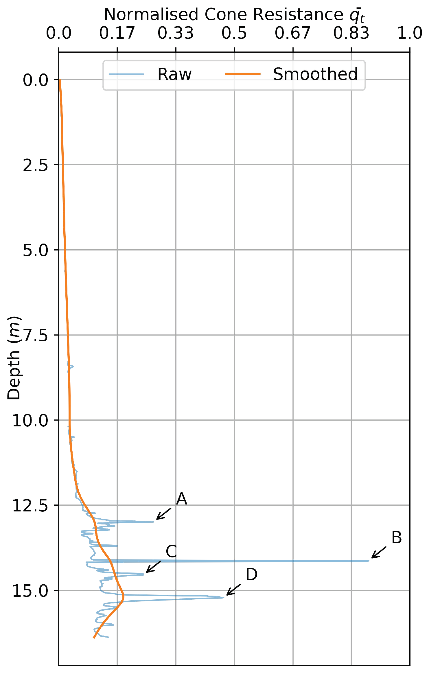
Some of the peaks in the CPT data have physical significance. To demonstrate this, the raw data for the corrected cone resistance from the first location marked by S. No 1 is plotted in Figure 2. It shows several peaks, and the more pronounced peaks have been labelled A, B, C and D. It can be also be seen in the raw values of Figure 2, that there is significant stochasticity within the corrected cone resistance values. The slight variations observed to a depth of 11 m are classified as noise, simply because the model is unable to predict these spikes, so we will treat them as white Gaussian noise.
A, B, C and D moreover, are not outliers or background noise. They signify the presence of a thinner layer of differing geotechnical character. Typically, geotechnical engineers observe the overall character of the CPT profile and use averaging techniques, as discussed by Alshibli et al. [29].
To remove the scatter (hereon referred to as noise within the CPT), and take into account the resistivity change, as indicated by the peaks, univariate cubic splines [32] were used. Other non-parametric approaches, such as kernel regularisation [33] and z-score [34] to remove outliers, were also investigated. However, those approaches were unable to fully generalise the trend and showed significant susceptibility to the local variability. Using wider window margins to suppress the effect of sudden peaks would cause the algorithm to develop a poor fit, and hence the techniques were dropped in favour of the univariate cubic splines. Figure 2 provides a side-by-side comparison of the two techniques employed to reduce the noise. Kernel smoothing (left) shows that it adapts well to the overall profile, giving a lower MSE compared to the cubic spline smoothing (right). However, the latter technique shows that it is able to reduce the overall stochasticity within the data, and provides a better averaged fit by filtering out the noise. Kernel smoothing shows that it is susceptible to local changes, and was therefore dropped in favour of cubic spline smoothing.
The cubic spline f reduces the function given in Equation (1). The first term is the error measure and the second is a roughness measure. The term D 2 f gives the second derivatives for the function f. The smoothing parameter p varies between 0 and 1; 0, as the smoothing parameter produces a spline with a least-squares straight line fit, whereas 1 is a natural cubic spline interpolant. The code used for univariate cubic splines is an adaptation of de Boor’s algorithm [35]. This algorithm is used through CSAPS which is a Python-based library that implements this algorithm and provides a convenient API for end-users.
Each one of peaks A, B, C and D in Figure 2 indicates a sharp change in soil properties, highlighting the increase of heterogeneity with depth. For instance, peak A is a single local maximum, however for the next few meters, the cone registers an increased resistance. This indicates soil type variation, and necessitates that the information be captured in the smoothing spline. Thus, we see a transition in q t from 0.08 to 0.17 . Peak B presents an interesting phenomenon. Although q t @ B is greater than q t @ A, the smoothed spline seems to plateau off near B and rises only around C to D. This can be understood if the general spread over peaks B, C and D is analyzed. From the graph, it is evident that peak B represents a single data point, whereas peaks C and D show a much wider depth range over which subsequent readings of q t showed an increased value.
This information is therefore captured in the smoothing spline by controlling the smoothness parameter. It should however, be noted here that due to the absence of ground truth and engineering judgement, the smoothed out curve follows the principles of statistical averaging.
p j = 1 n w j | y j f ( x j ) | 2 + ( 1 p ) λ ( t ) | D 2 f ( t ) | 2 d t
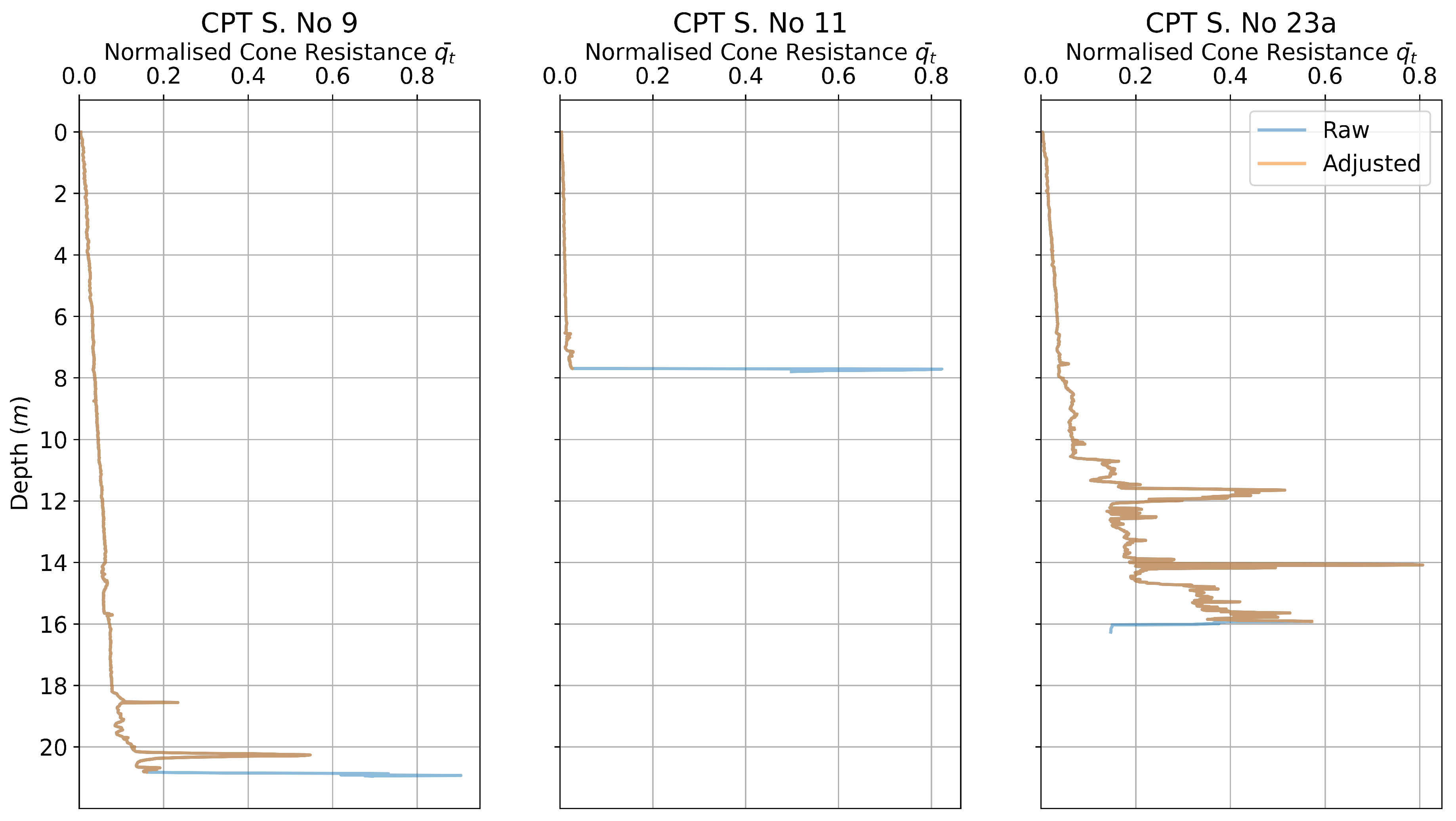
To smooth out data from the 24 different locations, custom smoothing factors were used. The smoothing factor was varied between 0.1 and 0.9 . For three sites however, records of high resistance values corresponding to CPT refusal were not fully filtered during data cleaning, and had to be removed here. This was encountered in three locations, and the data has therefore been adjusted, as shown in Figure 3. The model fed into the network is represented by the orange trend line labelled ‘Adjusted’ in the figure.

3.3. Excluding CPT Data for Shallow Gas Affected Locations

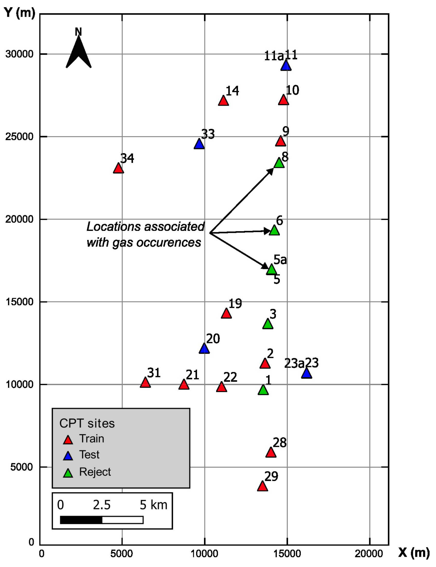
The presence of a shallow gas accumulation in the sub-surface is known to have an effect on CPT parameters (e.g., Coughlan et al. [17]). As shown in Figure 4, some of the CPT profiles (5, 5a, 6a and 8) were performed in and around regions where shallow gas was present. Even though the map shows only four locations where shallow gas is present, CPT data indicate its possible permeation to the neighbouring site CPT 3. Unfortunately, free gas can only be mapped on seismic data when the concentration is significant enough [36,37,38]. Hence, free gas occurrence here may extend outside the mapped gas pocket [17], but at a lower concentration.
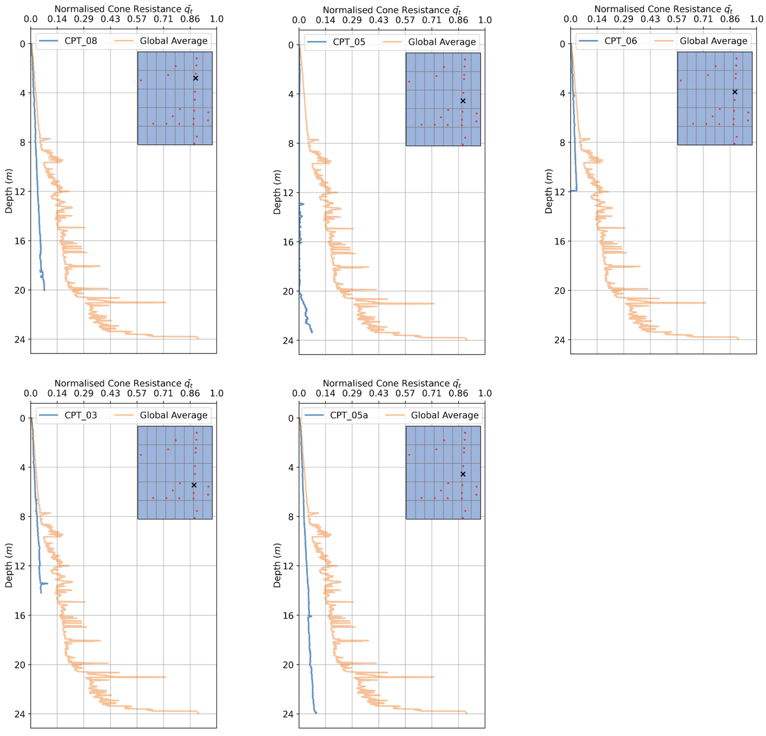
As the gas is likely to affect CPT records [39,40], Figure 5 shows the five CPTs (3, 5, 5a, 6 and 8) that had to be excluded from the dataset (at four locations, because CPT 5 and CPT 5a were at the same site). There are two fundamental problems with these five locations that were likely to affect the network. Firstly, CPT performs poorly in the presence of free gas. The results obtained from the tests carried into the different units affected by the occurrence of free gas do not display the same geotechnical behaviour as in the location free of gas. Hence, training datasets picked at the location affected by gas are likely to reduce the reliability of the overall predictions, and must be considered as a separate type of unit. Secondly, the range of values presented in each of these locations is three standard deviations out. This is especially true as the probe goes deeper into the seabed. The network is unable to generalise the trend and marks the data as outliers, effectively filtering the particular data point out—an intrinsic property of a neural network. More specifically, neural networks are prone to making unpredictable mistakes if they encounter out-of-distribution sample points [41].

3.4. Outputs

The target features in the neural network upon which predictions are made are the corrected cone resistance and sleeve friction. The former is the force experienced by the cone. Each value of q t corresponds to a specific depth value. The latter is the sleeve friction ( f s ). Similar to q t , it is associated with the depth value. Whilst pore pressure is an important parameter, it shows significant variability, unpredictability and poor repeatability, making it an unrealistic target feature. It is worth noting though that whilst significant independent depth data points and by extension q t and f s are present, 24 locations were actually investigated; and therefore, only 24 coordinate and bathymetry data are available.
To extend the coordinate and bathymetric information for each location to all of its corresponding depth points, Gaussian white noise is added to the coordinates and bathymetry. However, a total of 42,000 depth data points and corresponding cone and sleeve resistance data are available. To map the inputs onto the outputs, and provide each cone and sleeve resistance an output value with corresponding input features, the noise is added to the latitude, longitude and bathymetry input features so that these three features can be extended to the whole data range. This is necessary because feeding the neural networks’ constant values for the three input features across a large number of depth data points would inform the network that these play little to no role in output selection, and would therefore be blocked out of the network through gradient descent. To keep these input features relevant, noise to the order of 10 5 and 10 8 were added to the coordinates and bathymetry, respectively. The order of magnitude was determined as three orders higher than the precision of the input features. This imbalance is typical for real systems and has been observed frequently [42,43].

3.5. Data Normalisation

The range of values for each one of the input and output features is different. The diverse ranges that each of the inputs has would cause the weight calculation to skew in their favour simply due to the order of difference in their magnitude. This imbalance is typical for real systems and has been observed frequently [44,45,46]. The goal of making the importance of the features comparable is making each feature equally important—at least at the zeroth iteration of the forward propagation. Two choices are available to normalise the features:
  • Z-Score normalisation: Z-score normalisation [47] is carried out via calculating the mean and standard deviation of the data, and then adjusting every point using them. The mathematical formula to complete this is given in Equation (2). If a value of the feature is exactly equal to the mean, the new normalised value will come out to be zero. If it is below the mean, it obtains a negative value, and if it is above the mean, it obtains a positive value;
    n e w = v a l u e μ σ
  • Min-max scalar normalisation: This is one of the simplest ways to normalise the data. For a given range of data, the minimum value takes the value of 0 and the highest value takes the value of 1. Every other value is then transformed into a floating point number between these two bounding integers. Mathematically [48], this is achieved via the Equation (3).
    n e w = v a l u e m i n m a x m i n
Z-score normalisation deals with outliers better than the min-max scalar. However, it does not scale features to exactly the same scale. In this particular case though, the outliers were already treated via smoothing spline, as discussed in Section 3.2. Therefore, min-max scalar transformation was chosen as the method of normalisation, since it scales down every feature to the same scale. Other techniques, such as log scaling and clipping exist; however, min-max scalar transformation serves the purpose as data smoothing was already applied prior to feature scaling.

3.6. Machine Learning

The architecture of an ANN can be broken down into four components—hidden layers, neurons in each hidden layer, activation function for each neuron and finally the training algorithm that determines the overall weights and biases of the neurons in the network [49].
The input and the output layers are the only two layers that have a definite existence, so as to present and extract data from the network. The number of neurons in each of these two layers is determined quite simply by the number of input features for the input layer and the output features in the output layer.
Hidden layers located between the input and the output layers are ascribed weights and biases that force the input through an activation function at each neuron to derive an output, allowing for the non-linear transformation of the inputs. Hidden layers vary depending on the activation function applied to its neurons and on the overall architecture of the network.
While there is no theoretical approach to deciding on the possible number of hidden layers in a network, the optimum number is achieved heuristically. Making a network too deep may perform better on training datasets, but its accuracy can potentially drop on testing data because of over fitting [50,51]. Additionally, deeper networks need significantly more data to generalise well and they are computationally intensive [52]. Therefore, a balance has to be struck between the computational cost, training accuracy and testing accuracy. Beginning with shallow networks and progressively increasing the depth is thus recommended for maximising the performance against computational parsimony.
A neuron or a node is a memory-less connection point in a NN. They are characterised by synaptic weights and biases representing the connection between the preceding and the subsequent layers of input and output. NNs have a layered architecture and within each layer, one or more nodes exist. As new input-output information is received, the weights and biases at each node change to adjust to this new information, and that is how learning occurs. When a neuron receives and processes information, it decides whether an output should be passed to the next layer as input. The decision to pass it onward is determined by the activation function built into the neuron.
In neural networks, activation functions are used to introduce non-linearity into the network [53]. In the absence of activation functions, every neuron will only be performing linear transformation on the inputs using the weights and biases, making the number of hidden layers irrelevant because each layer will be making the exact same calculation. This would make the model into a simple linear regression model. Activation functions decide whether a neuron will be activated or not. In simpler terms, it determines whether the neuron’s input to the network is important in order to obtain the given outputs from the inputs, using simple mathematical operations. It transforms the summed weighted inputs from the node into an output, and feeds it into the next hidden layer or to the output layer. The choice of activation function depends on the data that are available, the functionality expected and the required output.
This paper has established the need for non-linear approaches to determine the soil resistivity with location and depth. Therefore, neurons with non-linear activation functions, e.g., sigmoid and ReLU are used in the hidden layers.
Ultimately, this is a regression analysis. Therefore, the activation functions on the output layer that then gives the required features at the end of an analysis, has a linear activation function. The non-linearity within the system is catered to by the non-linear activation functions imposed on the hidden layers, and the output layer translates this into the required output feature.
ReLU and the slightly modified leakyReLU activation functions were used in the architecture. ReLU and leakyReLU activation functions are represented in Equations (4) and (5), respectively.
f ( x ) = 0 , if x 0 x , if x > 0
f ( x ) = α x , if x 0 x , if x > 0
where f ( x ) is the output of the neuron after the activation function is applied to the input x. x is the output of the preceding layer. α is the leak in the leakyRelu activation function.
Preference was given to ReLU and its derivative over the sigmoid or Tanh type activation function because:
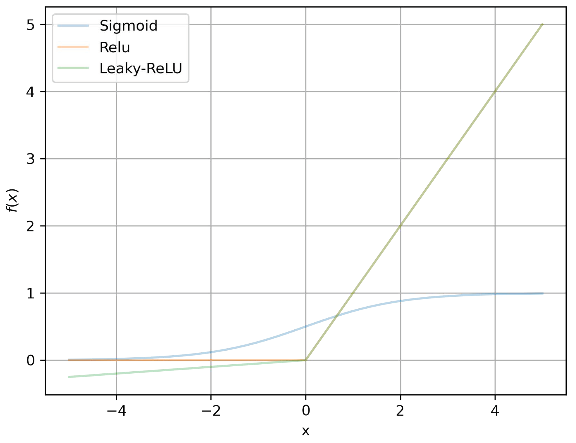
  • Vanishing gradients: This is a problem encountered while training ANNs with gradient-based learning methods and back propagation. During each iteration of the learning process, the NN’s weights at each neuron are updated proportionally to the partial derivative of the error function, with respect to the current weight. In the worst case scenario, the gradients become vanishingly small, bringing the training process to a virtual halt, i.e., the value of the weight does not change because the partial derivative is infinitesimally small. This holds for non-linear activation functions, such as sigmoid or hyperbolic tangent, as shown in Figure 6 towards the edges of the function, where the derivative is close to zero but not zero. Their gradients are within the range of 0 and 1, and because back propagation computes gradients via the chain rule, multiplying these very small gradients for an n layered system, the gradients would drop exponentially with n, and the first couple of layers would train very slowly [54];
  • Sparsity: Sparse matrices are matrices in which most of the elements are zero. Since negative input values generate a zero output, the resulting matrix is a simpler matrix with true zero values, instead of vanishingly small non-zero values. This prevents some neurons from activating in a particular layer. This has several advantages in itself. Deactivating several neurons in every layer makes the learning process faster. This in turn, causes the network’s predictive accuracy to improve by preventing over fitting [55].
Still, ReLU has some disadvantages. It can suffer from exploding gradient—a problem in direct contradiction with the vanishing gradient. When significant cost or errors accumulate during training, the resulting weights become too large, making the model too unstable. Another problem that ReLU can experience is that of a dying ReLU. We can see in Figure 6 that for the ReLU function, any input less than zero always produces a zero output. It is then improbable that a neuron can recover once it has become inactive. Such neurons are then useless to the overall network, and are said to be dead. LeakyRelu mitigates the pitfalls of using ReLU by introducing a leak in the function. This leak can be seen in Figure 6 for the values x < 0 where the function now has a slope greater than 0. The smaller slope ensures that the neurons where the input is negative never die and have a chance of eventually waking up.
Additional adjustments, such as batch normalisation or clipping or gradient clipping were not required at this stage, as the LeakyReLU utilised in the NN showed no sign of exploding gradient. Table 2 summarises the properties of the linear and non-linear activation functions.
Finally, it is important to highlight the nature of the activation function that ought to be used for the output layer. This particular problem falls under the domain of supervised learning. Supervised learning is a branch of deep learning that makes use of labelled datasets that, in this particular case, translate into datasets that have corresponding outputs for a set of inputs. As the input data are fed into the NN, the weights are adjusted until the model has been fitted appropriately. This appropriation of a model occurs as part of the process termed cross validation. To build an ANN, the following sequence of events takes place:
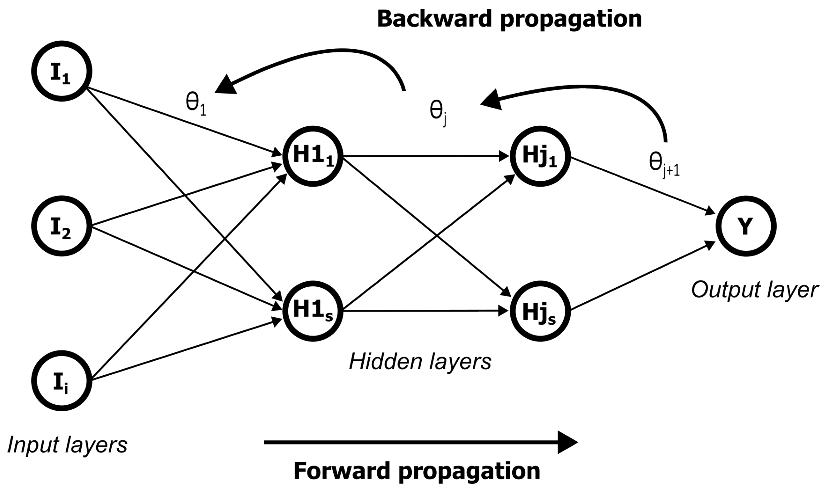
  • Weights and/or bias initialisation: Each synapse-connection between two neurons in successive layers has a weight associated with it. This weight multiplies itself with the input from the previous layer, if there is any, and calculates the result of the activation function. This is then fed as the input to the next layer. If a network has s j neurons in the j t h layer, and s j + 1 neurons in the j + 1 layer, then θ j will be of dimension s j × s j + 1 , where θ j is a matrix holding the weights that control the function mapping from layer j to j + 1 . Weights can be initialised, either as zero or randomly. Zero initialisation can cause the NN to enter into a state of symmetry, and prevent efficient learning. Every subsequent iteration will then be the same for the network since the derivative, with respect to the loss function, will be the same. Random initialisation is preferred. However, there is a chance that random initialisation might assign weights that may be too small or too high, that would then give rise to vanishing or exploding gradients. While vanishing gradients can be accounted for by using a ReLU-type activation function, it can still suffer from exploding gradients. Biases however, need not to be randomly initialised and can be set to zero;
  • Forward propagation: This step is shown in the solid lines that move from left to right in Figure 7. Forward propagation can be further broken down into two sub-steps. The first is the pre-activation. Pre-activation is the weighted sum of inputs, i.e., linear transformation of inputs using weights calculated either from the random initialisation in the first pass or the adjusted weights after the back propagation step. Based on this aggregated sum, and after routing this sum through the activation function, the neuron makes a decision on whether this information is passed on to the next layer or not. The second constituent step of the forward propagation is the activation. The weighted sum of inputs are passed on to the activation function from the pre-activation step. The two equations below give the forward propagation step using the following two equations:
    z = h ( x ) = θ T x g ( z ) = m a x ( α z , z )
    z here signifies the pre-activation step that is calculated using the linear weighted sum of inputs. θ is the weights for the specific layer in question. g is the activation function, the leaky-ReLU;
  • Cost/Error function: A penalty term to assist the network in training the weights, so as to minimize the overall network cost in making a prediction. In supervised learning, the actual output for a set of input features is known. Therefore, by comparing the output with the input, and calculating the overall error within the network, the weights can be adjusted in the forward propagation step to improve accuracy. The cost function used here is the mean square error given by the following equation:
    1 2 m Σ ( h ( x i ) y i ) 2
    Notice how the equation makes use of the term h ( x ) instead of g ( z ) —the output of every hidden layer is indeed g ( z ) , barring the output layer. Since this is a regression problem, the final set of neurons in the output layer does not route the pre-activation sum through the activation function. Therefore, the comparison of the network output h ( x ) is made through the actual result y;
  • Backward propagation to adjust the weights and/or biases: Back propagation is the right to left pass shown in the dashed grey lines in Figure 7. In essence, it makes use of the cost function to adjust the weights. Properly tuning the weights and biases allow for reduced errors. To reduce the errors, a method called gradient descent is used. Gradient descent is a numerical method to calculate the differential increase or decrease in the cost function with respect to the weight. It computes the gradient of the loss function for each weight using the chain rule.
    θ j = θ j β θ j J ( θ j )
    θ j is the weight that is being adjusted. The second term is the penalty term obtained from the cost differential that provides the direction and magnitude for the penalty. β is the learning rate that, for the purpose of this study needs not be adjusted, since the optimiser used for the network is the ADAM optimiser [56].
Finally, the regularisation used for the network is termed the elastic net. Elastic net combines both the lasso (L1) and ridge (L2) regularisation, thereby, overcoming the shortcomings of the L1 and L2 techniques. The hyperparameters for these were fine tuned using several iterations that will be covered in the next section.
A percentage split of 72-8-20% was used for the training validation test split. The testing sites were manually selected to ensure non-homogeneity of the selection. Figure 4 shows the locations that were used in the training and testing of the network.

3.7. Hyperparameter Tuning

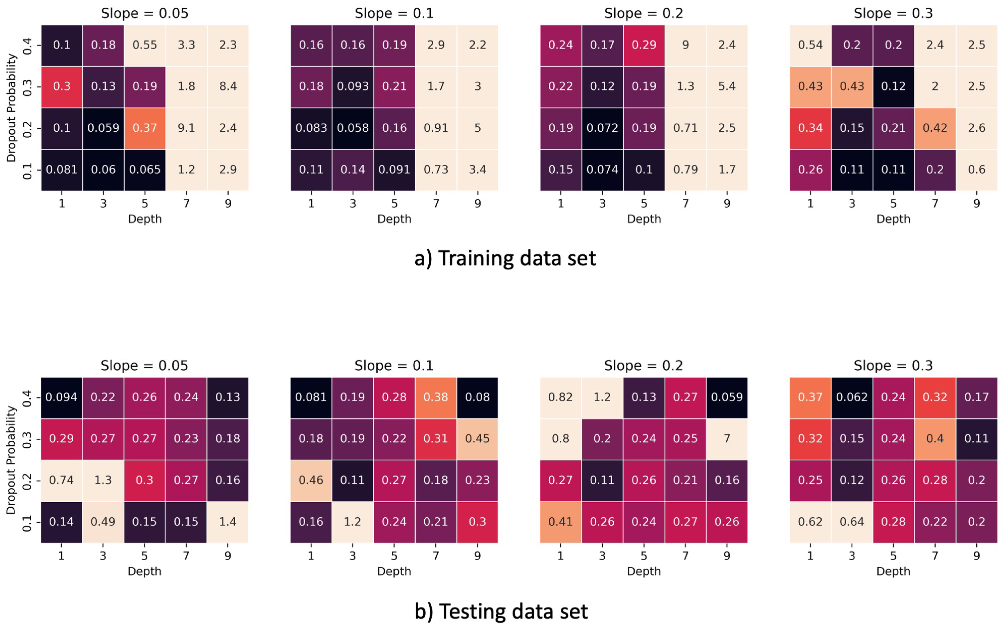
To determine the optimum set of hyperparameters for the network, the depth and width of network, leak or slope of the activation function and regularization are determined iteratively. The results of the hyperparameter tuning are shown in Figure 8. The results of the iterations on the training dataset show that extremely shallow networks with less than five hidden layers tend to perform better than relatively deeper networks. Increasing the depth beyond five layers negatively influences the predictability of the network too. This holds true for all four different slope values in question, and for testing and training datasets. Results from the testing dataset are inconclusive.
The performance metric used for this study is the mean squared error (MSE) [57,58,59] that compares the average of the squared difference between the true value and the predicted value, as per Equation (6) where y i is the true value and y i ^ is the predicted value of the cone resistance or sleeve friction.
M S E = 1 N i = 1 N ( y i y i ^ ) 2

4. Results

4.1. Training Neural Network

The training phase of the ANN is a key step that conditions the precision and accuracy of the CPT parameter predictions. Because the ANN in this study has been trained on a limited input dataset, there is no associated and conclusive information on the geological units these CPTs were performed on, and there is no definitive methodology to conclude that the training validation test split takes into account all of the different geological units present within the 330 k m 2 area of the site (see Section 2). Hence, the topic physics-assisted training validation test split could not be covered in this study. This could also be a major reason why the testing data show lower MSE values compared to those of the training dataset, as seen in Figure 8. However, all of the data within the testing set were ensured to be near the existing CPTs in the training data. As such, the probability of the network encountering unseen geology is less.
As this particular application cannot be treated simply from a statistical point-of-view, the physics of geology have to be considered. To that effect, the locations for the training and testing datasets were hand-picked. The main criteria for selecting the test sites was their nearness to existing clusters of data. CPTs performed near each other are likely to share the same succession of stratigraphic units (see Section 2 for the stratigraphic units description). This increases the likelihood of achieving similar cone resistance values. In fact, in this sector of the Irish Sea, the variations within the stratigraphic units essentially occur at broader scales [17]. Only the occurrence of local heterogeneity, internal to units, could diminish the likelihood of achieving a similar corrected cone resistance. Such occurrences are likely to happen in the heterogeneous units, such as glacio-marine and till sediment units. However, the shallowest mud and sand units are characterised by relatively homogeneous sediment facies over the stratigraphic model extent from Coughlan et al. [17], and are thus unlikely to exhibit local heterogeneity. Moreover, spikes visible on the CPT profiles related to these potential variations within units have been smoothed during the dataset preparation (see Section 3.2), and are therefore considered irrelevant here. Out of the 24 locations for which the results were available, five were discarded because the data showed effects from shallow gas [17]. Hence, the sediment layers affected by the presence of gas are likely to display another pattern of CPT response while being of the same unit and same sediment type. This left 19 locations, with 15 of them assigned to the training dataset. The latter were all ensured to be on the outer boundaries of the site.
The four locations that were marked for test verification were ensured to be in line with the local clusters of the training sites (Figure 4). For instance, site 20 is carefully selected because it is in line towards the north-west and south-west by CPT sites. Moreover, it is bounded by two additional CPT sites towards its south-east and east. This makes it an excellent test site. Sites 11a and 23a might pose as the outlier to this rule described above. However, they were selected because repeat CPTs were performed for these locations. Figure 4 shows three such CPTs, as 5a, 11a and 23a, in addition to 5, 11 and 23. The former set represents the repeated measurements to a greater depth compared to the latter set. The latter set has data measurements to a relatively shallower depth below the seabed, when testing had to be terminated due to technical issues with data acquisition. This repeated measurement is taken at a location within 20 m of the original intended location. Therefore, it provides a good opportunity to test the NN. This also explains the relatively lower MSE recorded in the testing set compared to that of the training set.
To highlight the degree of unpredictability in seabed sub-surface geology, and potential pitfalls of using geographical nearness as a criterion for determining testing and training data sites, note site labelled 2 (Figure 4). Towards the north and south of this site, gaseous sub-layers are thought to be present; the shallow gas occurrence has only been evidenced north of this location, based on geophysical datasets [17]. Geographically, the northern and southern CPT sites are nearer to site 2. The western and eastern flanks of this site are marked by sites 20 and 23, respectively (Figure 4), both of which do not present any indication of the presence of gaseous sub-layers. Still, site 2 defies the in line geological trend that presents itself as soil-based stratification below seabed.
The site located north of site 2 may, in fact, be affected by the occurrence of gas outside the mapped gas pocket [17]. According to Davis [38] and more recently, Kim et al. [37], the occurrence of free gas within sediments may not be observed on geophysical data if concentration is too low. However, it could still affect the sediment properties [38,60], and hence influence the CPT data [39,40]. Secondly, the unpredictability of the site 1 south of site 2 may be related to the CPT unit behaviour. While the inclination of the CPT unit rarely exceeds 4 over the whole area, the inclination at site 1 exceeds 7 . This is likely to affect the CPT data, and hence reduce the likeliness of geotechnical profiles with the other sites, leading to its exclusion.
In comparison to other studies, Syn-CPTs generated with the support of geophysical data better capture the variability of CPT parameters in varying soil units. However, most of these studies have been performed in environments with relatively well stratified and often homogeneous stratigraphy with depositional environments, and sequence clearly identified (e.g., marine, fluvial, lacustrine or estuarine). In fact, in the marine units of the Irish Sea (muds and silts), the models developed in this study perform quite well, both in terms of statistical (MSE) and physical interpretation. The models’ performances start to decrease when entering the more heterogeneous units, interpreted as glacial deposits characterised by heterogeneous sediments, such as cobbles, gravels and sand clasts in a stiff fine-grained matrix. Still, the CPT parameters’ values range observed within these units (i.e., 0–28 M Pa for q t ) are lower than the values observed for other depositional environments mentioned before (e.g., 0 to 50 M Pa in Sauvin et al. [9]), and here, they only occur as spikes. Hence, one can consider that the variations of soil behaviour type are even harder to discriminate in the complex glacial sediment deposits of the Irish Sea.
Considering the limited amount of input parameters (lack of support from geophysics at this point of development), the accurate prediction of CPT parameters for the shallowest (marine) units, and relatively accurate prediction in the glacial units (U3 and U4), the model developed in this study has some potential for ground modelling studies during wind farm developments. An interesting point to consider is the CPT parameter range accessible through the different model predictions. While the prediction of one model can potentially be endlessly discussed compared to the reality, the CPT parameter values range could be a good indicator of the potential soil behaviour type. In fact, considering the different models explored in this study, capturing the broad scale evolution of the CPT parameters could help to qualitatively discriminate the soil units.

4.2. Model Performances

The heat maps in Figure 8 provide a summary of which model performs better than the rest. While shallower networks (depths up to five) show superior performance on the training datasets, their performance gives mixed results for the testing sets. This can be attributed to the limited number of sample locations and the relative proximity of these sample locations to the training locations, causing high levels of homogeneity in the geotechnical properties. Proceeding with the set of parameters that gives the lowest MSE on the testing data, is unfortunately not the best course of action due to the limited number of data points available. Therefore, a different strategy was adopted. Global errors were calculated by combining both the training and testing datasets. Their true values were compared with the predicted values and the global mean square errors were calculated. The resulting heat map from this arrangement are shown in Figure 9.
It can be observed from Figure 9 that deeper networks tend to be worse off than the shallower networks across different values of slopes. A similar trend is also seen in the magnitude of slopes with comparatively smaller values outperforming larger values. Slopes of 0.05 and 0.1 almost always outperform larger values of slopes, as long as depth remains less than seven.
The network that gives the lowest MSE is considered to be the best performing network, and in this case, the lowest observed MSE as read-off from Figure 9 is 0.067 . This is observed when the depth is 3, the dropout is 0.2 and the slope is 0.1 . Some other sets of hyperparameters also give a low MSE, but they are above 0.7 , and hence this is considered to be the best model.

Prediction Using NN

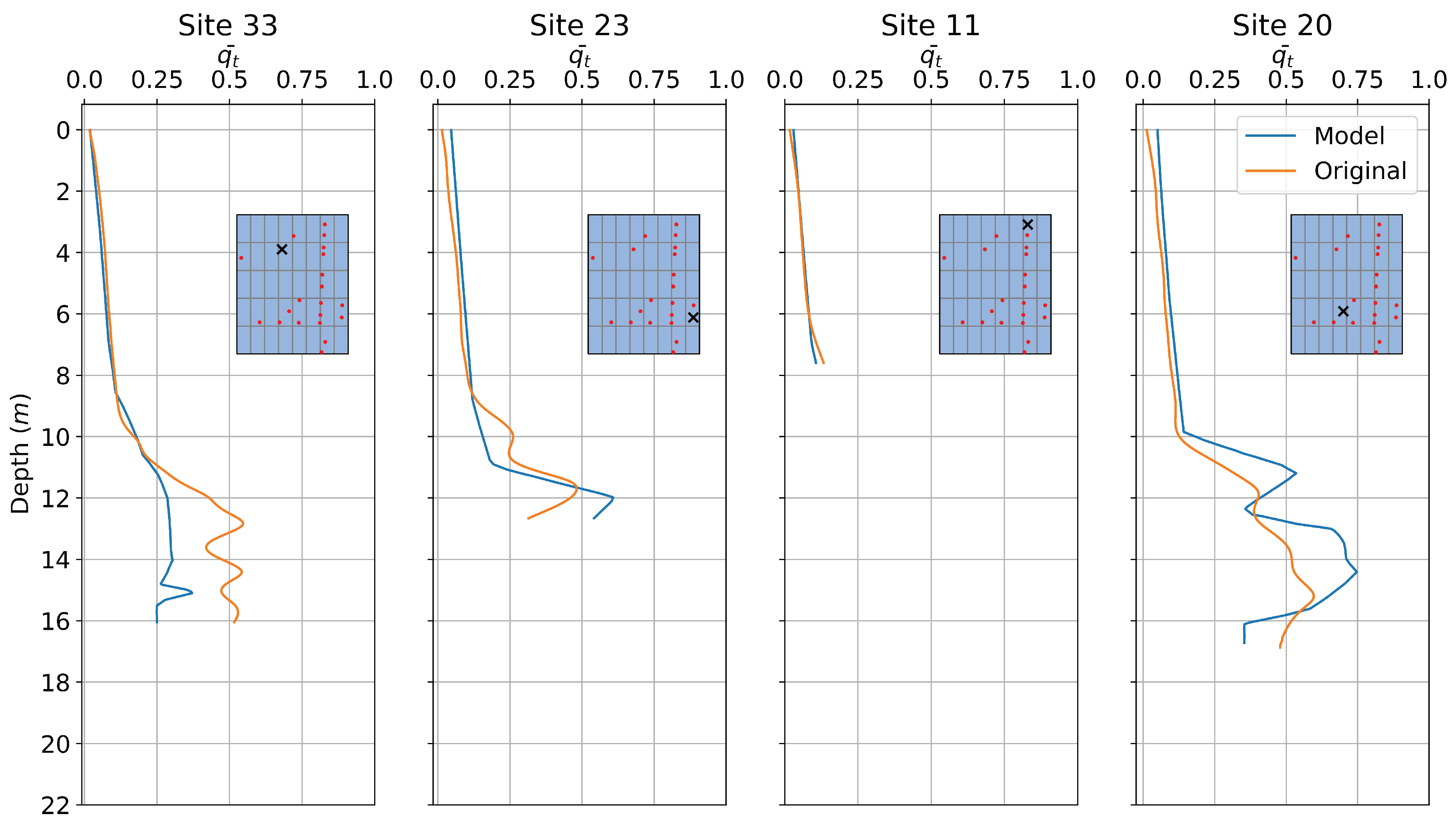
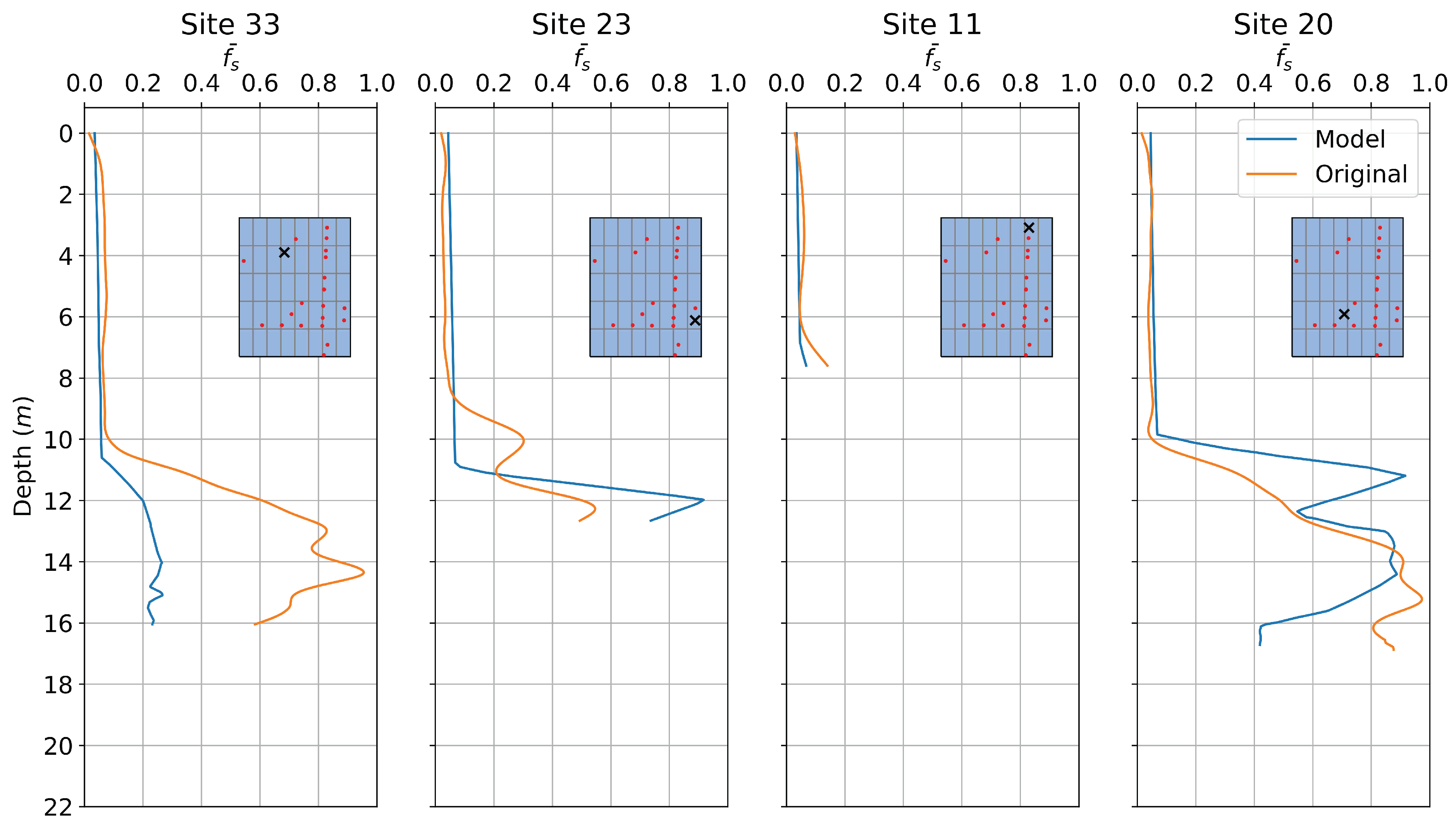
The model predictions for shallow sub-sea depths, when compared to higher subsea depths, are relatively more accurate where the geological units do not undergo rapid evolution in their properties, as seen from the original profiles of cone resistance in Figure 10 and Figure 11. In fact, the model quite accurately mimics the gentle increase in q t up to depths of 10 m for all four test sites. It should be noted that the model, without exception, does tend to slightly over-predict the q t for all four sites.
The responsiveness of the model to increase in resistance beyond the 10 m depth is inconclusive (Figure 10). For sites 33 and 20, the model is early to predict the rise in q t by approximately 0.5   m . The true resistance values lag behind the ones predicted by the model. The jump experienced by site 20 however, is much more radical, compared to that of 33. Although, this may be a reflection of the gradient of evolution of cone resistance in that geological unit. The true resistance value also sees a very sudden jump that is unlike the one observed at site 33. For the remaining two sites, 23 and 11, the model lags the true value in its prediction, and only starts to register an increase after around 0.5   m .
Sudden changes by definition cannot be known by automatic data analysis, since it has not been encountered before. Moreover, over time, it can only learn from these events if they have a distinct signature. However, the sharp changes happen over a small/sudden depth, and consequently it is very hard to have a distinct signature pattern that can be formed. Consequently, AI can establish the anomaly, but in realistic conditions, such as these, qualitative interpretations or non-AI interpretations based on physics are often required to classify and characterise the anomaly. This is the type of interaction that is required for such systems, over a complete autonomy of AI.
Apart from site 11 that terminates in still shallow sub-seabed depth, the other three sites provide interesting, but contrasting results. In greater depths, the variation in geological units is significant, as seen from the true values themselves in Figure 10. Site 33, beyond the 10 m mark, constantly under-predicts the cone resistance. It does show an increase in line with the true values. This increase however, does not have as strong a gradient as that of the true resistance profile. It also fails to show any localised variations in resistance in the shape of the local maxima and minima, as the original profile undergoes. This is likely due to the inherent nature of statistical systems to be relatively non-responsive to quick or sudden changes. Around the 15 m mark, it does however, register a slight crest before falling down again, just as the original profile does. The magnitude of the change is higher for the model than it is for the original profile.
Site 23 in Figure 10 continues its flatter trajectory despite the rise seen in the original values after around 9 m . The gradient the model has remained rather the same from what it was in the shallow sub-seabed depth. It is only after 11 m that the model registers an increase following an increase in the true profile. This increase however, causes the model to over predict.
Site 20 in Figure 10 almost always over-predicts the q t , even at greater sub-seabed depths, which is unlike any of the other three results observed. Whilst it increases in magnitude following the trend of the original profile, the increase is significantly larger than the true increase, causing the model to overshoot. Around 12 m where the original profile experiences a slight dip in resistance values, the model observes a significantly large dip as well before rising again to uncharacteristically larger resistance values. For this particular site, the model proved to be over-responsive.
The conclusion drawn for q t from Figure 10 is also valid for f s in Figure 11, except for the shallow sub-seabed depth behavior. Unlike the q t values predicted by the model in Figure 10, the f s predictions in Figure 11 at shallow depths are under-predicted and appear to be almost constant throughout up until 10 m , where there is some change observed. Of course, the consistency in predicted f s appears to be in line with the one in the original profile. The only other distance in the prediction quality between f s and q T is the magnitude (or scale) of these two particular properties, as q t is measured and predicted in M Pa , while f s is measured and predicted in k Pa .

5. Conclusions

There is a growing need for offshore ground investigation and characterisation related to wind farm development to be made more efficient and cost-effective. This will involve deriving enhanced value from fewer, more targeted investigations at specific locations using tools, such as cone penetration testing (CPT). In this study, machine learning was used as a tool to augment the ground investigation efforts for an offshore area where the sub-surface geological structure comprised shallow, relatively homogeneous geological units and deeper, more heterogeneous deposits.
These types of deposits represent different geological conditions previously investigated using synthetic CPT generation. To spatially predict CPT values with depth, artificial neural networks (ANNs) proved a good alternative to conventional statistical techniques that cannot necessarily be used because their underlying mathematics assume the problem to be linear in nature, or they can not handle the high sparsity.
Shallow neural networks with depths less than seven predicted artificial CPT data with lesser mean squared errors. Neural networks trained on CPT data need hyperparameter tuning for the activation function parameters (in this case, the slope of the LeakyRelu), depth and the regularization parameter to achieve optimum results. The lowest recorded MSE on cone resistance with optimised hyperparameters was 0.067 . The model performed well on shallow, homogeneous deposits, but struggled to capture and predict the lateral variability within the more heterogeneous, glacial deposits. Furthermore, the occurrence of shallow gas within the extent of the studied area had to be considered separately, as the CPT records affected by the presence of gas showed a different soil behaviour.
Potential pitfalls of using machine learning for an offshore site with inhomogeneous sub-seabed geological units are discussed and suggestions made to navigate these pitfalls. Aside from the geotechnically heterogeneous deposits, shallow gas in the sub-surface also complicates the use of ANNs or any statistical technique for interpolation, as the resistance does not follow the general trend observed in any geological unit, throwing off the network. These results highlight the limitations that the current generation of AI has. Use of reinforcement learning here might be justified; however, that requires access to additional data and sourcing that is cost-prohibitive. Likewise, to counter the high variability within the CPT profiling itself, spline smoothing was used to increase the predictive accuracy of the neural network.
Reinforcing ANNs with geophysics to convert this network into a physics-informed neural network would likely increase the efficacy of this network significantly. However, this requires supplementary data from multi-channel seismic profiling that may not always be available, and requires additional processing expertise. At present, as a result of the inconsistencies in output against real-world data, the use of machine learning to generate Syn-CPT is preferable for early stage conceptual studies and site characterisation rather than full front-end engineering design. The data may also be used to guide survey campaign planning, helping to define target location to investigate during later stages of development.

Author Contributions

G.S.: Conceptualisation, Methodology, Formal analysis, Writing—original draft, Visualisation. G.M.: Conceptualisation, Methodology, Formal analysis, Writing—original draft, Visualisation. M.C.: Resource, Conceptualisation, Writing—review and editing. A.M.: Resource, Conceptualisation, Writing—review and editing. I.T.: Resource, Conceptualisation, Writing—review and editing. V.P.: Conceptualisation, Methodology, Writing—review and editing, Visualisation, Supervision, Project administration, Funding. C.D.: Resource, Conceptualisation, Writing—review and editing, Supervision, Project administration, Funding. All authors have read and agreed to the published version of the manuscript.

Funding

This project received funding through the Sustainable Energy Authority of Ireland (SEAI) under their Research, Development and Demonstration Funding Program 2019 (Award: 19/RDD/439). This paper contains Irish Public Sector Data (INFOMAR) licensed under a Creative Commons Attribution 4.0 International (CC BY 4.0) licence. Mark Coughlan and Cian Desmond received funding through the Marine Institute Ship-Time Program for survey work carried out under CE22002.Vikram Pakrashi would like to acknowledge the Science Foundation Ireland funded NexSys (21/SPP/3756), Enterprise Ireland SEMPRE and SEAI funded REMOTEWIND RDD/613 and TwinFarm RDD/604. Gohar Shoukat and Vikram Pakrashi would like to acknowledge the funding EBPPG/2021/108 from Irish Research Council.

Acknowledgments

The authors would like to thank Irish Research Council to fund this doctoral research into use of artificial intelligence in offshore wind design under the Employment Based Post Graduate Program, in partnership between University College Dublin and Gavin and Doherty Geosolutions.

Conflicts of Interest

The authors declare no conflict of interest.

Abbreviations

The following abbreviations are used in this manuscript:
S. NoSerial Number
NNNeural Network
ANNArtificial Neural Network
CNNConvolution Neural Network
ReLURectified Linear Unit
CPTCone Penetration Tests
Syn-CPTSynthetic Cone Penetration Testing
RMSERoot Mean Square Error
MSEMean Square Error

References

  1. European Commission.Boosting Offshore Renewable Energy for a Climate Neutral Europe. Available online: https://ec.europa.eu/commission/presscorner/detail/en/ip_20_2096 (accessed on 20 March 2023).
  2. Barrett, M.; Farrell, N.; Roantree, B. Energy Poverty and Deprivation in Ireland; ESRI Research Series 144; The Economic and Social Research Institute: Dublin, Ireland, 2022. [Google Scholar]
  3. Forsberg, C.; Lunne, T.; Vanneste, M.; James, L.; Tjelta, T.; Barwise, A.; Duffy, C. Stothetic CPTS from Intelligent Ground Models Based on the Integration of Geology, Geotectoics and Geophysics as a Tool for Conceptual Foundation Design and Soil Investigation Planning. In Proceedings of the Offshore Site Investigation Geotechnics 8th International Conference Proceeding, London, UK, 12–14 September 2017; Society for Underwater Technology: London, UK, 2017; Volume 1254, pp. 1254–1259. [Google Scholar]
  4. Lunne, T.; Powell, J.J.; Robertson, P.K. Cone Penetration Testing in Geotechnical Practice; CRC Press: Boca Raton, FL, USA, 2002. [Google Scholar]
  5. Remy, N.; Boucher, A.; Wu, J. Applied Geostatistics with SGeMS: A User’s Guide; Cambridge University Press: Cambridge, UK, 2009. [Google Scholar]
  6. Arshid, M.U.; Kamal, M.A. Regional Geotechnical Mapping Employing Kriging on Electronic Geodatabase. Appl. Sci. 2020, 10, 7625. [Google Scholar] [CrossRef]
  7. Robertson, P.K.; Cabal, K.L. Guide to Cone Penetration Testing for Geotechnical Engineering; Gregg Drilling & Testing, Inc.: Martinez, CA, USA, 2015. [Google Scholar]
  8. Goovaerts, P. Geostatistics for Natural Resources Evaluation; Oxford University Press on Demand: Oxford, UK, 1997. [Google Scholar]
  9. Sauvin, G.; Vanneste, M.; Vardy, M.E.; Klinkvort, R.T.; Forsberg, C.F. Machine Learning and Quantitative Ground Models for Improving Offshore Wind Site Characterization. In Proceedings of the OTC Offshore Technology Conference, Houston, TX, USA, 6–9 May 2019. [Google Scholar]
  10. Carpentier, S.; Peuchen, J.; Paap, B.; Boullenger, B.; Meijninger, B.; Vandeweijer, V.; Kesteren, W.V.; Erp, F.V. Generating synthetic CPTs from marine seismic reflection data using a neural network approach. In Proceedings of the Second EAGE Workshop on Machine Learning, Onine, 8–10 March 2021; Volume 2021, pp. 1–3. [Google Scholar]
  11. Phoon, K.K.; Zhang, W. Future of machine learning in geotechnics. Georisk Assess. Manag. Risk Eng. Syst. Geohazards 2022, 17, 7–22. [Google Scholar] [CrossRef]
  12. Liakos, K.G.; Busato, P.; Moshou, D.; Pearson, S.; Bochtis, D. Machine Learning in Agriculture: A Review. Sensors 2018, 18, 2674. [Google Scholar] [CrossRef] [PubMed]
  13. Rauter, S.; Tschuchnigg, F. CPT Data Interpretation Employing Different Machine Learning Techniques. Geosciences 2021, 11, 265. [Google Scholar] [CrossRef]
  14. Erdogan Erten, G.; Yavuz, M.; Deutsch, C.V. Combination of Machine Learning and Kriging for Spatial Estimation of Geological Attributes. Nat. Resour. Res. 2022, 31, 191–213. [Google Scholar] [CrossRef]
  15. Vardy, M.E.; Vanneste, M.; Henstock, T.J.; Clare, M.A.; Forsberg, C.F.; Provenzano, G. State-of-the-art remote characterization of shallow marine sediments: The road to a fully integrated solution. Surf. Geophys. 2017, 15, 387–402. [Google Scholar] [CrossRef]
  16. Michel, G. Photograph of Geomil Manta-200 CPT during CE22002 Survey; Geomil Equipment: Westbaan, The Netherlands, 2022. [Google Scholar]
  17. Coughlan, M.; Wheeler, A.; Dorschel, B.; Long, M.; Doherty, P.; Mörz, T. Stratigraphic model of the Quaternary sediments of the Western Irish Sea Mud Belt from core, geotechnical and acoustic data. Geo-Mar. Lett. 2019, 39, 223–237. [Google Scholar] [CrossRef]
  18. Belderson, R.H. Holocene sedimentation in the western half of the Irish Sea. Mar. Geol. 1964, 2, 147–163. [Google Scholar] [CrossRef]
  19. Jackson, D.I.; Jackson, A.A.; Evans, D.; Wingfield, R.T.R.; Barnes, R.P.; Arthur, M.J. The Geology of the Irish Sea; British Geological Survey: Keyworth, UK, 1995; p. 133. [Google Scholar]
  20. McCabe, A.M. Glacial Geology and Geomorphology: The Landscapes of Ireland; Dunedin Academic Press: Edinburgh, Scotland, 2008. [Google Scholar]
  21. Chiverrell, R.C.; Thrasher, I.M.; Thomas, G.S.; Lang, A.; Scourse, J.D.; van Landeghem, K.J.; McCarroll, D.; Clark, C.D.; Cofaigh, C.Ó.; Evans, D.J.; et al. Bayesian modelling the retreat of the Irish Sea Ice Stream. J. Quat. Sci. 2013, 28, 200–209. [Google Scholar] [CrossRef]
  22. Dickson, C.; Whatley, R. The biostratigraphy of a Holocene borehole from the Irish Sea. In Proceedings of the 2nd European Ostracodologists Meeting, London, UK, 23–27 July 1993; British Micropalaeontological Society: London, UK, 1993; pp. 145–148. [Google Scholar]
  23. Michel, G.; Coughlan, M.; Arosio, R.; Emery, A.R.; Wheeler, A.J. Stratigraphic and palaeo-geomorphological evidence for the glacial-deglacial history of the last British-Irish Ice Sheet in the north-western Irish Sea. Quat. Sci. Rev. 2023, 300, 107909. [Google Scholar] [CrossRef]
  24. Coughlan, M.; Long, M.; Doherty, P. Geological and geotechnical constraints in the Irish Sea for offshore renewable energy. J. Maps 2020, 16, 420–431. [Google Scholar] [CrossRef]
  25. Bishop, J.M. Artificial intelligence is stupid and causal reasoning will not fix it. Front. Psychol. 2021, 11, 513474. [Google Scholar] [CrossRef]
  26. Buckley, T.; Ghosh, B.; Pakrashi, V. A Feature Extraction & Selection Benchmark for Structural Health Monitoring. Struct. Health Monit. 2022, 22, 2082–2127. [Google Scholar]
  27. Eslami, A.; Moshfeghi, S.; MolaAbasi, H.; Eslami, M.M. 6—CPT in foundation engineering; scale effect and bearing capacity. In Piezocone and Cone Penetration Test (CPTu and CPT) Applications in Foundation Engineering; Eslami, A., Moshfeghi, S., MolaAbasi, H., Eslami, M.M., Eds.; Butterworth-Heinemann: Oxford, UK, 2020; pp. 145–181. [Google Scholar]
  28. Rogers, D.; PE, R. Fundamentals of Cone Penetrometer Test (CPT) Soundings; Missouri University of Science and Technology: Rolla, MO, USA, 2020. [Google Scholar]
  29. Alshibli, K.; Okeil, A.; Alramahi, B.; Zhang, Z. Reliability Analysis of CPT Measurements for Calculating Undrained Shear Strength. Geotech. Test. J. 2011, 34, 721–729. [Google Scholar]
  30. Kordos, M.; Rusiecki, A. Improving MLP Neural Network Performance by Noise Reduction. In Theory and Practice of Natural Computing; Dediu, A.H., Martín-Vide, C., Truthe, B., Vega-Rodríguez, M.A., Eds.; Springer: Berlin/Heidelberg, Germany, 2013; pp. 133–144. [Google Scholar]
  31. Penrod, C.; Wagner, T. Another Look at the Edited Nearest Neighbor Rule; Technical report; Texas University at Austin Department of Electrical Engineering: Austin, TX, USA, 1976. [Google Scholar]
  32. Yu, L.; Jin, Q.; Lavery, J.E.; Fang, S.C. Univariate Cubic L1 Interpolating Splines: Spline Functional, Window Size and Analysis-based Algorithm. Algorithms 2010, 3, 311–328. [Google Scholar] [CrossRef]
  33. Hastie, T.; Tibshirani, R.; Friedman, J. Kernel smoothing methods. In The Elements of Statistical Learning; Springer: Berlin, Germany, 2009; pp. 191–218. [Google Scholar]
  34. Rose, P. Considerations in the normalisation of the fundamental frequency of linguistic tone. Speech Commun. 1987, 6, 343–352. [Google Scholar] [CrossRef]
  35. De Boor, C.; De Boor, C. A Practical Guide to Splines; Springer: New York, NY, USA, 1978; Volume 27. [Google Scholar]
  36. Öz Yilmaz. Seismic Data Analysis: Processing, Inversion, and Interpretation of Seismic Data; Society of Exploration Geophysicists: Houston, TX, USA, 2001; p. 2092. [Google Scholar]
  37. Kim, Y.J.; Cheong, S.; Chun, J.H.; Cukur, D.; Kim, S.P.; Kim, J.K.; Kim, B.Y. Identification of shallow gas by seismic data and AVO processing: Example from the southwestern continental shelf of the Ulleung Basin, East Sea, Korea. Mar. Pet. Geol. 2020, 117, 104346. [Google Scholar] [CrossRef]
  38. Davis, A. Shallow gas: An overview. Cont. Shelf Res. 1992, 12, 1077–1079. [Google Scholar] [CrossRef]
  39. Sultan, N.; Voisset, M.; Marsset, T.; Vernant, A.M.; Cauquil, E.; Colliat, J.L.; Curinier, V. Detection of free gas and gas hydrate based on 3D seismic data and cone penetration testing: An example from the Nigerian Continental Slope. Mar. Geol. 2007, 240, 235–255. [Google Scholar] [CrossRef]
  40. Steiner, A.; Kopf, A.J.; Henry, P.; Stegmann, S.; Apprioual, R.; Pelleau, P. Cone penetration testing to assess slope stability in the 1979 Nice landslide area (Ligurian Margin, SE France). Mar. Geol. 2015, 369, 162–181. [Google Scholar] [CrossRef]
  41. Luan, S.; Gu, Z.; Freidovich, L.B.; Jiang, L.; Zhao, Q. Out-of-Distribution Detection for Deep Neural Networks With Isolation Forest and Local Outlier Factor. IEEE Access 2021, 9, 132980–132989. [Google Scholar] [CrossRef]
  42. Geron, A. Handson Machine Learning with Scikitlearn; Keras & TensorFlow o’Reiley Media Inc.: Sebatopol, CA, USA, 2019. [Google Scholar]
  43. Momeny, M.; Neshat, A.A.; Hussain, M.A.; Kia, S.; Marhamati, M.; Jahanbakhshi, A.; Hamarneh, G. Learning-to-augment strategy using noisy and denoised data: Improving generalizability of deep CNN for the detection of COVID-19 in X-ray images. Comput. Biol. Med. 2021, 136, 104704. [Google Scholar] [CrossRef] [PubMed]
  44. Mohamed, M.M.; Schuller, B.W. Normalise for Fairness: A Simple Normalisation Technique for Fairness in Regression Machine Learning Problems. arXiv 2022, arXiv:2202.00993. [Google Scholar]
  45. Kissas, G.; Yang, Y.; Hwuang, E.; Witschey, W.R.; Detre, J.A.; Perdikaris, P. Machine learning in cardiovascular flows modeling: Predicting arterial blood pressure from non-invasive 4D flow MRI data using physics-informed neural networks. Comput. Methods Appl. Mech. Eng. 2020, 358, 112623. [Google Scholar] [CrossRef]
  46. Wu, H.; Köhler, J.; Noé, F. Stochastic normalizing flows. Adv. Neural Inf. Process. Syst. 2020, 33, 5933–5944. [Google Scholar]
  47. Schober, P.; Mascha, E.J.; Vetter, T.R. Statistics from a (agreement) to Z (z score): A guide to interpreting common measures of association, agreement, diagnostic accuracy, effect size, heterogeneity, and reliability in medical research. Anesth. Analg. 2021, 133, 1633–1641. [Google Scholar] [CrossRef]
  48. Eliazar, I.; Metzler, R.; Reuveni, S. Universal max-min and min-max statistics. arXiv 2018, arXiv:1808.08423v1. [Google Scholar]
  49. Wang, S.C. Artificial neural network. In Interdisciplinary Computing in Java Programming; Springer: Berlin, Germany, 2003; pp. 81–100. [Google Scholar]
  50. Salman, S.; Liu, X. Overfitting mechanism and avoidance in deep neural networks. arXiv 2019, arXiv:1901.06566. [Google Scholar]
  51. Zhang, C.; Bengio, S.; Hardt, M.; Recht, B.; Vinyals, O. Understanding deep learning (still) requires rethinking generalization. Commun. ACM 2021, 64, 107–115. [Google Scholar] [CrossRef]
  52. Hestness, J.; Ardalani, N.; Diamos, G. Beyond human-level accuracy: Computational challenges in deep learning. In Proceedings of the 24th Symposium on Principles and Practice of Parallel Programming, Washington, DC, USA, 16–20 February 2019; pp. 1–14. [Google Scholar]
  53. Hornik, K.; Stinchcombe, M.; White, H. Multilayer feedforward networks are universal approximators. Neural Netw. 1989, 2, 359–366. [Google Scholar] [CrossRef]
  54. Tan, H.H.; Lim, K.H. Vanishing Gradient Mitigation with Deep Learning Neural Network Optimization. In Proceedings of the 2019 7th International Conference on Smart Computing & Communications (ICSCC), Miri, Malaysia, 28–30 June 2019; pp. 1–4. [Google Scholar]
  55. Glorot, X.; Bordes, A.; Bengio, Y. Deep Sparse Rectifier Neural Networks. In Proceedings of Machine Learning Research, Proceedings of the Fourteenth International Conference on Artificial Intelligence and Statistics, Ft. Lauderdale, FL, USA, 11–13 April 2011; Gordon, G., Dunson, D., Dudík, M., Eds.; PMLR: Fort Lauderdale, FL, USA, 2011; Volume 15, pp. 315–323. [Google Scholar]
  56. Bae, K.; Ryu, H.; Shin, H. Does Adam optimizer keep close to the optimal point? arXiv 2019, arXiv:1911.00289. [Google Scholar]
  57. Willmott, C.J.; Matsuura, K. Advantages of the mean absolute error (MAE) over the root mean square error (RMSE) in assessing average model performance. Clim. Res. 2005, 30, 79–82. [Google Scholar] [CrossRef]
  58. Poli, A.A.; Cirillo, M.C. On the use of the normalized mean square error in evaluating dispersion model performance. Atmos. Environ. Part A Gen. Top. 1993, 27, 2427–2434. [Google Scholar] [CrossRef]
  59. Gupta, H.V.; Kling, H.; Yilmaz, K.K.; Martinez, G.F. Decomposition of the mean squared error and NSE performance criteria: Implications for improving hydrological modelling. J. Hydrol. 2009, 377, 80–91. [Google Scholar] [CrossRef]
  60. Seifert, A. In Situ Detection and Characterisation of Fluid Mud and Soft Cohesive Sediments by Dynamic Piezocone Penetrometer Testing. Ph.D. Thesis, Universität Bremen, Bremen, Germany, 2011. [Google Scholar]
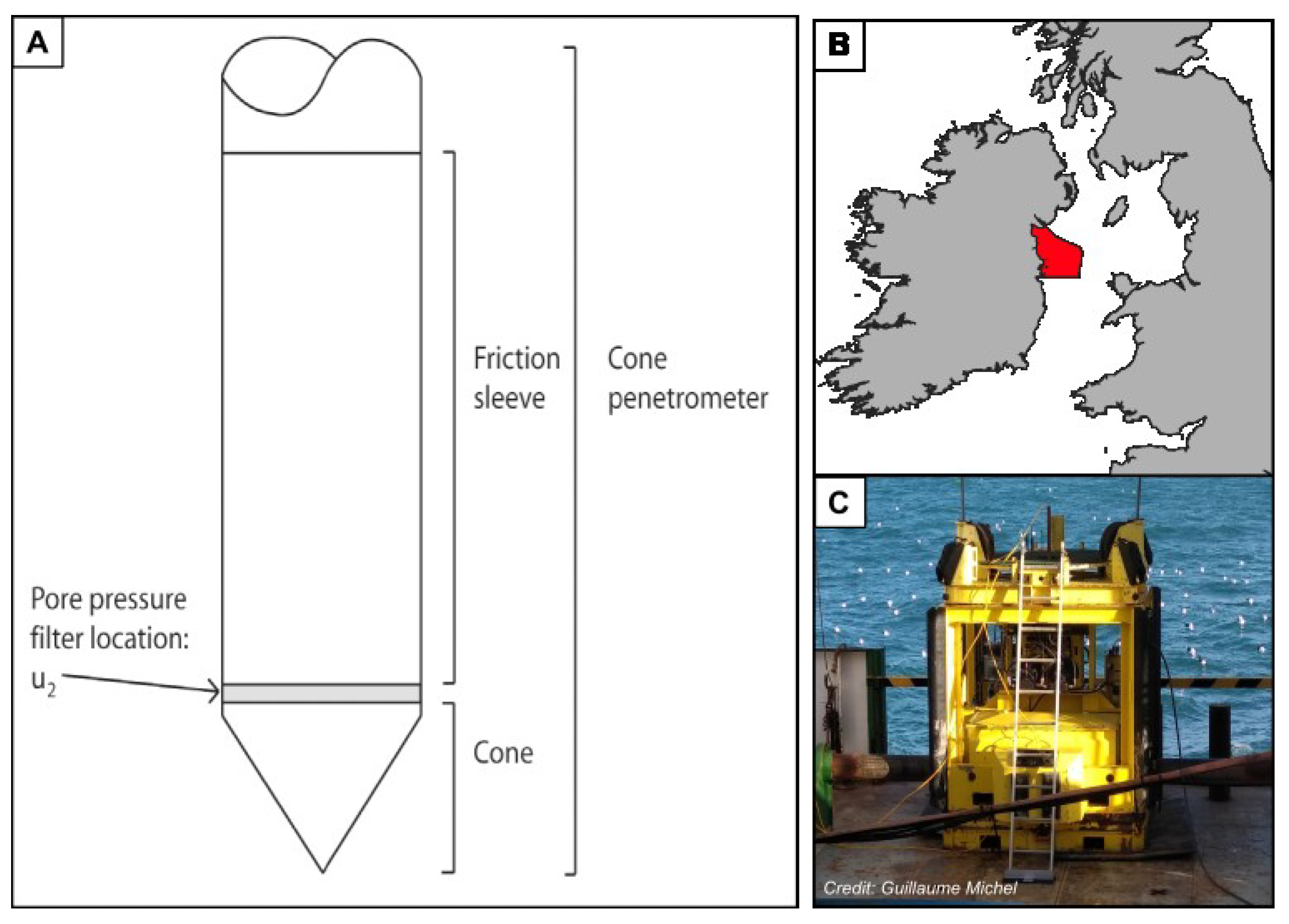
Figure 1. (A) Schema of a standard cone penetrometer (adapted from [7]), (B) a general location map of the study area in the Irish Sea and (C) a picture of the Geomil Manta-200 CPT acquisition system during the CE22 002 survey (Picture Credits: Guillaume Michel) [16].
Energies 16 03817 g001
Figure 2. Raw CPT data against the depth obtained directly from the tests compared with the smoothed out data after filtering was applied. The data are obtained from CPT S. No 1. Image on the left shows the smoothed profile after kernel smoothing is applied and the image on the right shows the results of cubic spline smoothing. A–D are labels identifying the distinct peaks that, in theory, can indicate a plausible geomorphological change in the soil stratification, but without borehole data or seismic results, this is difficult to conclude. The results displayed are normalised using a min-max scalar transformation, as per Section 3.5.
Energies 16 03817 g002
Figure 3. Deletion of the end data points retained by the CPT database. The before and after results of the corrected cone resistance data for CPT S. No 9, 11 and 23a. The results displayed are normalised using a min-max scalar transformation, as per Section 3.5.
Energies 16 03817 g003
Figure 4. Site map showing the locations that were used for training the neural network and those that were used for testing the network. The red triangles represent the sites that fed data into the training dataset and the blue triangles represent the sites that fed data into the testing dataset. The green ones represent the locations that were suspected to have gaseous sub-layers, and so were discarded from the NN. Blue markers signify the location of the CPTs that form the test data. Nos 11 and 11a; 23 and 23a and 5 and 5a are three sites where more than one CPT was carried out. The multiple CPT markers at sites 11 and 23 overlap because the CPT locations are virtually the same, with a distance of approximately 18.5 m between the repeated CPTs. Site 2 represents the odd location that does not present gaseous sub-layers, unlike its neighbouring locations.
Energies 16 03817 g004
Figure 5. Corrected cone resistance values for the five locations where a gaseous sub-layer was encountered and plotted in comparison with the global depth average at each unit depth. The results displayed are normalised using a min-max scalar transformation, as per Section 3.5.
Energies 16 03817 g005
Figure 6. Graphical representation of the activation functions sigmoid, ReLU and LeakyReLU to allow for comparison between the three different activation function choices available.
Energies 16 03817 g006
Figure 7. Schematic of a generic neural network showing the connection between the neurons, input layer and the output layer. This particular example has two hidden layers, three input features and one output. The blue solid line highlights the forward propagation step of the algorithm and the black dashed line is the back propagation.
Energies 16 03817 g007
Figure 8. Heat map of the NN showing the corrected cone resistance q t MSE results obtained for a combination of different depths of network against the slope ( α ) parameter to adjust the leak in the LeakyReLU for the testing data. The results show the tuning of the depth of the NN and slope of the activation function. The annotations in each square represent the averaged MSE for that model. (a) shows the results of the MSE calculated from the different networks on the training data. (b) shows the results of the MSE calculated from the different networks on the testing data.
Energies 16 03817 g008
Figure 9. Heat map showing the MSE results for the corrected cone resistance q t obtained for a combination of different depths of the network against the slope ( α ) parameter to adjust the leak in the LeakyReLU for the testing data. The results show the tuning of the depth of the NN and slope of the activation function. The annotations in each square represent the averaged MSE for that model. The MSE here is calculated using the global dataset obtained by combining the training and testing datasets, and comparing their true q t values against the predicted values.
Energies 16 03817 g009
Figure 10. Comparison between the smoothed ground truth values of the corrected cone resistance against the predicted corrected cone resistance by the best model identified through heat-maps. The results displayed are normalised using a min-max scalar transformation, as per Section 3.5.
Energies 16 03817 g010
Figure 11. Comparison between the smoothed ground truth values of the sleeve friction against the predicted sleeve friction by the best model identified through heat-maps. The results displayed are normalised using a min-max scalar transformation, as per Section 3.5.
Energies 16 03817 g011
Table 1. Definition of the CPT parameters.
SymbolDefinitionFormula
Q c Total force experienced by the cone-
A c Total force experienced by the cone-
q c Cone resistance ratio of the total forcing acting on the cone to the projected area of the one Q c A c
F s Total force experienced by the friction sleeve-
A s Surface area of the friction sleeve-
f s Sleeve resistance ratio of the total force acting on the sleeve to the surface area of the sleeve F s A s
u 2 Pore pressure-
q t Corrected cone resistance ratio of the total force acting on the cone to the projected area of the sleeve with the correction of the pore pressure effects q t = q c + u 2 ( 1 A c )
f s ¯ Normalised sleeve friction by dividing the local value with the local maximum f s ¯ = f s max f s
q t ¯ Normalised corrected cone resistance by dividing the local value with the local maximum q t ¯ = q t max q t
Table 2. Summary of the comparison between the sigmoid, ReLU and LeakyReLU.
Activation Function
PropertySigmoidReLULeaky-ReLU
Range0–10–
Vanishing GradientsYesNoNo
NatureNon LinearLinearLinear
Zero CentredNoNoNo
Dying ReLU-YesNo
Computational ExpenseHighLowLow
Disclaimer/Publisher’s Note: The statements, opinions and data contained in all publications are solely those of the individual author(s) and contributor(s) and not of MDPI and/or the editor(s). MDPI and/or the editor(s) disclaim responsibility for any injury to people or property resulting from any ideas, methods, instructions or products referred to in the content.