Multi-Step Wind Power Forecasting with Stacked Temporal Convolutional Network (S-TCN)

Abstract

Nowadays, wind power generation has become vital thanks to its advantages in cost, ecological friendliness, enormousness, and sustainability. However, the erratic and intermittent nature of this energy poses significant operational and management difficulties for power systems. Currently, the methods of wind power forecasting (WPF) are various and numerous. An accurate forecasting method of WPF can help system dispatchers plan unit commitment and reduce the risk of the unreliability of electricity supply. In order to improve the accuracy of short-term prediction for wind power and address the multi-step ahead forecasting, this research presents a Stacked Temporal Convolutional Network (S-TCN) model. By using dilated causal convolutions and residual connections, the suggested solution addresses the issue of long-term dependencies and performance degradation of deep convolutional models in sequence prediction. The simulation outcomes demonstrate that the S-TCN model’s training procedure is extremely stable and has a powerful capacity for generalization. Besides, the performance of the proposed model shows a higher forecasting accuracy compared to other existing neural networks like the Vanilla Long Short-Term Memory model or the Bidirectional Long Short-Term Memory model.

1. Introduction

In recent years, rapid development in wind power generation has required more research in this field. Wind power generation has a high variability. Thus, reliable and accurate WPF methods can provide an important reference to the control of wind turbines and power system operations, such as unit scheduling, operation of energy storage systems, dispatch of transmission lines, and power system-related management.

Many up-to-date methods have been developed for predicting wind power generation. Reference [1] presents two types of wind power forecasting methods. The first category of methods is to predict the wind speed first and then use the predicted wind speeds and the power curve of wind turbines to predict wind power generation. The other strategy is to predict wind power generation directly; thus, it is not necessary to predict wind speeds first. Reference [2] classified the wind power forecasting methods into deterministic and probabilistic models. However, WPF can also be divided into ultra-short-term forecasts (a few seconds to 30 min ahead), short-term forecasts (30 min to 6 h ahead), medium-term forecasts (6 h to 1 day ahead), and long-term forecasts (1 day to 1 week ahead) according to the length of lead time [3].

Reference [4] introduces that WPF models can be classified into three main following types: physical models, statistical models, and artificial intelligence models. Physical models consider a variety of meteorological elements like numerical weather forecast (NWP)-based or measured temperature, humidity, and air pressure as the inputs of forecasting models [2]. Additionally, it is required for WPF to consider the contour, terrain, and barriers of an entire wind farm, as well as the power curve of wind turbines, to estimate wind speeds on the hub height. This method does not need large amounts of historical wind data. However, it is hard to model and analyze a variety of operating conditions, wind farm geographical environments, and atmospheric environments [2]. Traditional statistical models include the Hammerstein autoregressive model [5], fractional-ARIMA (f-ARIMA) [6], autoregressive moving average (ARMA) [7], and autoregressive integrated moving average (ARIMA) [8]. Typically, these time series models are used to analyze the linear variation in wind speed and wind power at different locations [1]. In order to create a mathematical model to describe the investigated time series, statistical models require a large amount of high-quality historical data [2]. In recent years, many deep learning algorithms have been used to make short-term predictions for wind power, and they have outperformed more conventional methods. For example, a long short-term memory network (LSTM) was designed to forecast time series in order to address the issue of gradient vanishing in RNNs [9]. In reference [10], a method for residual correction of wind speed forecast based on RNN was developed. In order to reduce the model’s training time, a gated recurrent unit network was also constructed by deleting some redundant LSTM structures [11,12].

Each WPF method has its advantages and weak points and is suitable for a particular objective or application. A Temporal Convolutional Network (TCN) architecture, in contrast to its predecessor, like Long Short-Term Memory (LSTM), can process long input sequences but require little memory during training [13]. TCN model has been developed for short-term WPFs, and it outperformed the other existing forecasting methods, such as Support Vector Machine (SVM), LSTM, GRU, and so on [14,15]. However, a traditional TCN approach only covers one-step-ahead wind power predictions. One-step-ahead wind power forecasting models, according to the literature [16], are insufficiently accurate to offer a stable and regulated operation. In comparison, multi-step-ahead forecasting has a number of application-based advantages as well as the ability to capture the full dynamics of wind power. These multi-steps ahead forecasting applications include power systems’ operation, control, economic dispatch, and unit commitment [17]. A comparison between the surveyed works is expressed in Table 1:

Table 1. Comparison between the surveyed works.

Ref.	Study Location	Used Technique/Method	Used Datasets	Performance Metrics	Pros	Cons
[4]	A wind farm in Shanghai	LSTM Networks, Similar Time Series and LightGBM	Wind power Generation and Meteorological factors (Wind direction, wind speed, and air temperature)	Root mean square error (RMSE) Mean absolute error (MAE) Mean absolute percentage error (MAPE)	➢ LSTM can consider the temporal correlation and effectively avoid the gradient disappearance and gradient explosion during the training stage ➢ LightGBM has the merits of preventing over-fitting, excellent generalization ability, faster speed, and lower memory consumption. ➢ The similar disparity can objectively compare the similarity between samples and reflect similar numerical values and trends.	➢ This reference only compared the proposed methods with ANN and SVM. The comparison is limited. ➢ The required dataset is too large, which increases the difficulty of model training. ➢ There is no data preprocessing for raw data.
[5]	Two sites (Site 01: Illinois 05245, site 02: New Jersey 07852)	Adapting Hammerstein (HAR) model to an Autoregressive approach	Wind speed	RMSE MAE MAPE	➢ The HAR model may be suitable for short-term (1–24 h) wind forecast predictions. It can capture various wind-speed characteristics, including asymmetric wind-speed distribution and non-stationary time series profile. ➢ The proposed method performs well compared to the classical time series model, such as ARIMA.	➢ This reference only considers wind speed prediction rather than wind power prediction. ➢ The required dataset is too large.
[6]	Wind generation sites in North Dakota	Fractional-ARIMA	Wind speed	Daily Mean Error (DME) Variance Forecast Mean Square Error (FMSE)	➢ The proposed method can improve the accuracy of forecasting compared to the persistence method.	➢ Forecasting errors below cut-in wind speed are ignored. ➢ The required dataset is too large. ➢ The reference needs to consider the market integration of wind farms and the systematic characterization of forecasting models.
[7]	NingXia, Heilong Jiang, He Bei, Guang Dong, Gan Su, and An Hui in China	➢ Non-parametric models: NP-NRC, NP-CV ➢ Machine learning models: ANN, SVN, RF ➢ Hybrid models: HAN-NRC, HAN-CV, HNA-NRC, HNA-CV, hybrid-BP-ARMA (HBA), hybrid-SVM-ARMA (HSA), hybrid-RF-ARMA (HRA)	Wind speed	MAE RMSE Mean Relative Error (MRE)	➢ This work compares the proposed non-parametric hybrid models with the single models and AI/ML models in wind speed forecasting and shows that the NP-based hybrid models generally have more robust forecast performances. ➢ In terms of the residuals from the NP fitting, the ARMA model is possible to obtain better prediction accuracy.	➢ This reference only considers wind speed prediction rather than wind power prediction.
[8]	Baltic Sea area	ARIMA	Wind speed	Autocorrelation coefficient (ACC)	➢ The proposed modified ARIMA modeling procedure works quite well in modeling wind-speed time-series data.	➢ This reference only considers wind speed prediction rather than wind power prediction.
[9]	Adelaide wind farm, located in Ontario, Canada	RNN model Lower upper bound estimation	The historical wind power data	PI coverage probability (PICP), PI normalized average width (PINAW), the index coverage width-based criterion (CWC), a new PI width evaluation criterion (PIMSE), a new CWC function (NCWC)	➢ The proposed RNN prediction model can construct better PIs compared to traditional benchmark models.	➢ As the forecasting lead time increases, the forecasting accuracy significantly decreases as a result of more uncertainties. ➢ The reference only considers one-step-ahead prediction.
[10]	A wind farm in the Ningxia Hui Autonomous Region of China	A framework that combines ICEEMDAN, BPNN, LSTM, GRU and ARIMA, and an error correction method based on ICEEMDAN-ARIMA.	Wind speed data at four sites	MAE RMSE MAPE	➢ The proposed method with error decomposition correction shows a good forecasting performance, and the method has a certain universality.	➢ The reference only considers one-step-ahead prediction. ➢ The reference only involves wind speed prediction instead of wind power prediction.
[14]	Wind farms in Taiwan	ANN LSTM XGBoost TCN	Historical wind power data and NWP wind speeds forecasted by Taiwan’s Central Weather Bureau	RMSE MAE	➢ This work compares four different methods in wind power forecasts and demonstrates that the XGBoost-based model would have the potential for short-term wind power forecasting.	➢ This work used local NWP wind-speed forecasts. These data cannot be applied to other areas.
[15]	A wind farm in the United States	TCN	Historical meteorological factors and wind power data	RMSE MAE	➢ The convergence speed of TCN is rapid, and the whole training process is stable. ➢ TCN has a strong generalization ability. ➢ TCN would be suitable for the short-term prediction of wind power generation.	➢ The reference only considers one-step-ahead prediction.
[16]	The Boco Rock Wind Farm in New South Wales, Australia	Dual-stage attention-based recurrent neural network (DA-RNN) Long and short-term time-series network (LSTNet) Temporal pattern attention-based long short-term memory (TPA-LSTM)	Historical wind speed and wind power data	RMSE MAE CV-RMSE	➢ This work compared three attention-based RNN models with the SVR, ELM, and RBF models. The results showed that the three attention-based RNN models have good performance for short-term wind power forecasts.	➢ The proposed attention-based RNN models could be less competitive when the time horizon increases.
[17]	National Renewable Energy Laboratory (NREL)	A deep learning model based on a dual-attention mechanism	The historical wind power, wind speed, wind direction, air density, and air pressure	MAE R2 Score Forecasting skill score (SS)	➢ The proposed model gives more weight to the input features while impacting more on the target values more. ➢ The proposed method may be suitable for other energy applications, such as demand-response forecasts or the prediction of charging and discharging loads.	➢ The proposed models require more parameters to be trained, which takes a long time, for model training and wind power forecasting.
[18]	A wind farm in North China	CEEMDAN-SVR-TCN	The historical wind power, wind direction, wind speed, environment temperature, impeller speed, converter speed measurement, generator speed, torque given, converter torque measurement, and blade torque	MAE RMSE MSE SSE	➢ The proposed method combines different machine learning methods to increase forecasting accuracy. ➢ The proposed method provides a reliable prediction result for short-term wind power prediction.	➢ The proposed method decomposes original wind power data, but the process of decomposition would reduce the extraction of important information on data.

Typically, the methods of wind power forecasting are classified into three main categories: physical models, statistical models, and artificial intelligence models. Physical methods consider a variety of meteorological elements like numerical weather prediction (NWP), wind speed, or irradiance. Physical methods can be applied for long-term forecasting; however, the forecasting results are also affected by the precision of numerical weather predictions. In this study, the NWP data were generated and owned by the Vietnam Meteorological and Hydrological Administration, which is confidential and makes the collection of NWP data more difficult. A similar situation would appear in other areas or countries. Thus, several international works also did not consider the inputs of NWPs. As for statistical and artificial intelligence-based models, the inputs of training models typically include important weather variables and historical measurements from wind farms to predict wind power generation. Thus, this study has collected meteorological and power generation data from the analyzed wind farm, including the measured wind power generation, temperature, wind speed, and wind direction. The main purpose of this study is to develop a robust multi-step forward wind power forecasting model that can deal with longer sequences, utilizing historical meteorological data and power generation.

Recently, a modified version of TCN called the Stacked Temporal Convolutional Network (S-TCN), has been developed. S-TCN has demonstrated a good performance in dealing with sequence problems in gene predictions [13] or anomaly detection in IoT. Therefore, this study has enhanced the existing S-TCN model for multi-step ahead wind power forecasting, and the historical measurements for wind speed and wind power were employed as input features. The main contributors of this paper include:

• This study modified the existing TCN by stacking multiple TCN layers that include causal dilated convolutions and residual connections to expand receptive fields and model longer time scales up to an entire sequence;
• This study aims to address a multi-step ahead forecasting for wind power using S-TCN, which was not developed by other works.

The rest of this paper is organized as follows: Section 2 introduces the principle of TCN and how to implement the S-TCN model for short-term wind power forecasting. Section 3 describes the process of short-term prediction for wind power. The proposed process includes data pre-processing, model training, and performance evaluation. Finally, Section 4 discusses the forecasting results using the proposed method for a study case. Section 5 summarizes the conclusions of this research.

2. Temporal Convolutional Network

2.1. Basic Principles of TCN

A TCN is a novel type of neural network based on a one-dimensional (1-D) convolutional neural network (CNN) [18]. TCN has a powerful extraction ability to analyze time series. In numerous industrial applications, including traffic estimation, audio processing, machine translation, and human motion detection, TCN has been shown to be superior to many deep learning algorithms, such as LSTM or GRU [19].

A typical TCN consists of three main parts: causal convolution, dilated convolution, and residual connections. First, the convolution in TCN has the causal ability, indicating that the output at a certain moment is only related to the present and historical inputs rather than the future inputs [18]. According to [20], a TCN was trained to predict the next $l$ values of the input time series. It is assumed that there is a sequence of inputs. $x_0, x_1,x_2,\dots x_L$, and the objective is to predict the corresponding outputs $y_0,y_1,y_2,\dots y_L$. At each time step, those values are related to the inputs that are shifted forward by $l$ time steps. Thus, when predicting the output $y_t$ for time step $t$, one can only use $l$ inputs: $x_{t-l+1},x_{t-l+2},\dots x_t$.

To meet the causal requirement, the first layer of TCN must be a fully convolutional 1-D network. Moreover, each intermediate layer has the same size as the input layer; then, the zero-paddings are executed, which makes the subsequent layers remain the same length as the previous ones. Figure 1 illustrates a model that has a basic causal convolution with one input layer, one output layer and two intermediate hidden layers. According to the structure of this figure, the output at time step t is only related to the inputs at time t, t − 1, t − 2, and t − 3 because the shifted time steps $l$ equal four. Besides, if we suppose that the filter is $F=\left(f_1,f_2,f_3,\dots f_l\right)$, the causal convolution of sequence $X=\left(x_1, x_2,x_3,\dots x_t\right)$ considered for the output at time step $t$ is shown as follows [18]:

$${\left(F\ast X\right)}_{\left(y_t\right)}={\displaystyle \sum }_{i=1}^l{f}_i{x}_{t-l+i}$$

(1)

where $\ast$ is the convolutional operation, and $\left(F\ast X\right)$ also means the output at time step $t$.

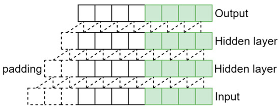
Figure 1. A causal convolutional with filter kernel size k = 2 and time steps shifted l = 4.

Moreover, the objective of TCN is to obtain an effective size of historical data for a long time. Thus, a large filter or an extremely deep learning structure would be required. Dilated convolutions are used to enable an exponentially large receptive field with limit layers to apply causal convolution on time series with a long history [21].

Figure 2 shows a model that has the causal and dilated convolutions with the same number of specific layers as the model in Figure 1. It is noticeable that there are more inputs of historical data relevant to the outcome at time step $t$ thanks to its dilated factors $d=1, 2, 4$. A dilated convolution has a filter that is applied over a region that is larger than its size by skipping input values with a given step. It augments some weights to the convolution kernel to make the input data to be unchanged, which leads to the increase in the size of the time series observed by the network [18]. The definition of dilated convolution is shown as follows [15]

$$F\left(s\right)=\left(x\ast f\right)\left(s\right)={\displaystyle \sum }_{i=0}^{k-1}f\left(i\right)x_{s-d·i}$$

(2)

where $\ast$ is the convolutional operation; d is the dilation rate; k is the size of the kernel, and $s-d·i$ is the past direction. When $d$ is one, dilated convolution has the state of ordinary convolution. Dilated convolutions enable the output to be affected by more nodes; therefore, it has a better performance for processing long time series. Some weights are added to the convolutional network to make the input data to be unchanged. Consequently, the size of the time series observed by the network is increased while the amount of computation remains unchanged [18].

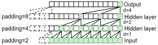
Figure 2. A dilated causal convolutional with dilated factors d = 1, 2, 4 and filter kernel size k = 3.

Moreover, to enable a larger TCN structure, it is important to stack a large number of layers and select a small filter’s size. The stack of the causal convolution and dilated convolutional network gradually make the number of layers of the neural network to be deeper. To avoid the problem of gradient attenuation or gradient decay, it is important to use the residual connections effectively for training deep networks [22]. To speed up the training process and avoid a vanishing gradient problem, the residual connections are integrated into the output layer of TCN. The input x is compensated into the output of the convolutional network as follows [15]:

$$o=Acitvation\left(x+F\left(x\right)\right)$$

(3)

where $F\left(x\right)$ is the output of the convolutional layer, and the rectified linear unit function is used as the activation function. This model can be trained more quickly and perform better thanks to the rectified linear activation function, which solves the vanishing gradient issue [23]. It is shown as follows:

$$f\left(x\right)=x^{+}=\max \left(0,x\right)=\left\{\begin{array}{c}1 if x>0\\ 0 if x\le 0\end{array}\right.$$

(4)

where $x$ is the input to a neuron.

During model construction, an entire residual module, which consists of several dilated causal convolutions, is executed. The TCN residual block structure is shown in Figure 3.

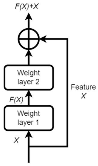
Figure 3. Structure of a residual module.

It can be seen that the residual module has a branch leading to a series of transform $F\left(X\right)$, whose output is added to the input $X$ of the block [24]. Residual connections effectively enable layers learning to alter the identity mapping as opposed to all transformation, which has repeatedly been shown to be advantageous to extremely deep networks.

2.2. Stacked Temporal Convolutional Network

To increase the forecasting accuracy by TCN, it is crucial to implement an extremely deep network or a large filter. The additional hidden layers recombine the learned representation from the previous layers and create new representations at high levels. Furthermore, many techniques can be used to alter TCN’s receptive fields, like stacking additional dilated convolutional layers, employing a greater dilation factor, or raising the size of the filter. In this study, the stacked temporal convolutional network was utilized for WPF. It is a novel TCN structure by stacking many networks to increase the complexity of computing results.

The number of filters in each TCN is selected in the same way to implement the CNN. Based on the ability of both computing hardware and matrix multiplication, the number of filters is usually designed to be two. Notably, the higher the number of filters, the more complex model is. However, the complexity of a model structure costs a lot of computation time.

This study applied a systematic approach to developing the forecasting model. In the first stage, the collected data were divided into three subsets: training, validation and testing sets. Next, the structure of S-TCN was designed and constructed. In the process of model construction, this work followed the following cycle: training, testing, evaluating, adjusting and repeating. The process of training and validation is expressed in Figure 4:

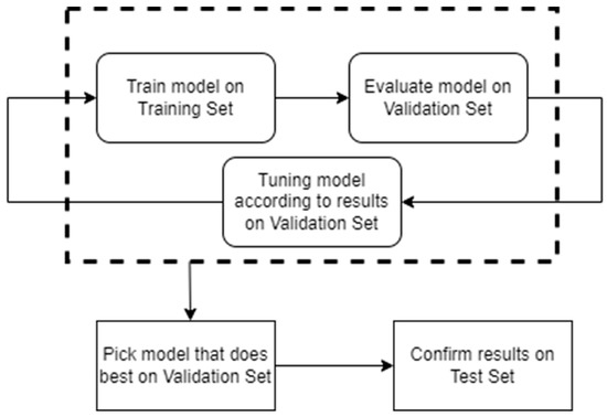
Figure 4. The training and validation process of the model.

First, the developed network was trained using the training set. The network was also optimized using the optimization algorithm (Adam) and the specified loss function when compiling the model. Then, the performance of the proposed network was evaluated on the validation set. This validation process helps the model designer tune the model’s hyperparameters and configurations accordingly. In this study, the model evaluation was performed on the validation set after every epoch. This work selected the structure of the respective hidden layers and the number of neurons based on a large number of experiments in our forecasting work. According to our experience with model training, few layers or neurons would cause underfitting. That is, underfitting could be caused when a complex data set is inputted to the training model with insufficient neurons or hidden layers, which would fail to detect the characteristics of signals accurately. In contrast, using an excessive number of neurons or hidden layers could lead to overfitting. That is, if the structure of the training model is enormous but the amount of input information is low, the model cannot be fully trained, which would cause overfitting. Moreover, an excessive number of neurons or hidden layers increases the required time to train the network. Therefore, in this study, the structure of the respective hidden layers with the corresponding neurons was determined based on the characteristics of the collected dataset in our analyzed wind farm. After many experiments, the S-TCN model can provide a better forecasting performance if each convolutional layer is in a residual block and 128 units of filters exist in the first hidden layer, as well as the rectified linear unit function is used as the activation function. Additionally, the kernel size is two, and the dilation rate is represented as a list including one, two, four, eight, 16, 32, and 64 for each internal hidden layer of the convolutional layer. To ensure a correct dimension of the output, the final layer of the proposed model utilizes a dense layer. It is a regular, deeply connected layer from its preceding layer, which works for changing the dimension of the output by performing matrix-vector multiplication. As a higher number of stacks of TCN is used, it requires a larger computation. Thus, training deep learning models will take a significant amount of time, especially for a complex model structure. In contrast, as a lower number of stacks of TCN is utilized, the model may be unable to capture the relationship between the input and output variables accurately, causing a high training or forecasting error. The architecture of the proposed model is expressed as follows:

In Figure 5, N is the number of stacked TCN layers experimented with, respectively, at two, three, four, and five.

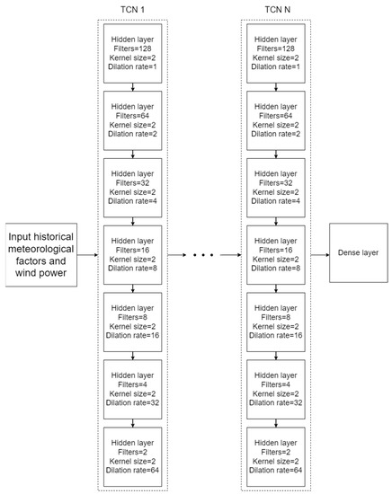
Figure 5. Stacked Temporal Convolutional Network (S-TCN).

3. Multi-Step Forecasting for Wind Power by S-TCN

3.1. Data Preprocessing

To examine the correlation of meteorological factors with wind power generation at each time step, the Pearson correlation coefficient (PCC) was used as follows [25].

$$r_p=\frac{{{\displaystyle \sum }}_{i=1}^n\left(x_i-x_{mean}\right)\left(y_i-y_{mean}\right)}{\sqrt{{{\displaystyle \sum }}_{i=1}^n{\left(x_i-x_{mean}\right)}^2}\sqrt{{{\displaystyle \sum }}_{i=1}^n{\left(y_i-y_{mean}\right)}^2}}$$

(5)

where $r_p$ is the PCC between the meteorological factor x and wind power generation y. Moreover, $x_{mean}$ and $y_{mean}$ are the mean of x and y, respectively.

Spearman Correlation Coefficient (SCC) is used as a nonparametric rank correlation metric to study the relationship strength between variables [26]. To use Spearman’s rank correlation coefficient, the data must be ordinal or continuous and follow a monotonic relationship. In a monotonic relationship between two variables, as one variable increases, the other variable tends to either increase or decrease, but not necessarily in a linear trend. That is, Pearson’s correlation assesses linear relationships, while Spearman’s correlation assesses monotonic relationships.

For a sample of size $n$, the $n$ raw scores $X_i,Y_i$ are converted to ranks $R\left(X_i\right),R\left(Y_i\right)$, respectively, and $r_s$ is computed as:

$$r_s=1-\frac{6\sum d_i^2}{n\left(n^2-1\right)}$$

(6)

where $d_i=R\left(X_i\right)-R\left(Y_i\right)$ is the difference between the two ranks of each observation, and n is the number of observations.

Spearman’s correlation coefficients range from −1 to +1. The sign of the Spearman correlation coefficient reveals whether the relationship is monotonic, positive, or negative. A positive correlation means that as one variable increases, the other variable tends to rise. A negative correlation indicates that as one variable increases, the other tends to fall. Values close to −1 or +1 represent a stronger relationship compared to values closer to zero.

In reality, the measurements of wind power generation would contain noises caused by manual operations, faults, maintenance, and so on. Thus, outlier detection is one of the critical tasks for data analyses. To remove the outliers of historical measurements, this work applied orange software to remove the outliers in the dataset by using a covariance estimator [27]. The Orange software provides a Python data mining library that can implement feature scaling, normalization, data cleaning, missing data imputation, and other functions [28]. This software was applied to detect outliers, as shown in Figure 6.

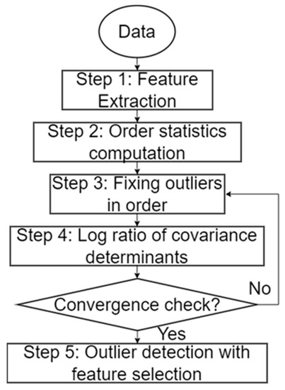
Figure 6. Covariance-based outlier detection with feature selection.

The meteorological data and wind power generation need to be normalized before the training of forecasting models. The process of normalization enables the loss function not to be converged [29]. In this study, the min-max normalization was used to transform the data into the values between [0, 1], which is represented as follows:

$$x^{\prime }=\frac{x-x_{min}}{x-x_{max}}$$

(7)

3.2. Training Model

After the data are preprocessed, the model is constructed with the parameters specified before. The model is completely trained when the set number of iterations is exceeded; while training models, we observe, monitor and recall precision to prevent overfitting. RMSE was used as the evaluation metric for calculating the accuracy of the model on the training and validation set.

3.3. Evaluating Forecasting Performance

For evaluating the performance of predictors, the common indicators, both root mean square error (RMSE) and mean absolute error (MAE), were used. RMSE is the square root of the average of the squared difference between the target value and the predicted value. In terms of MAE, it is the average of the differences between the ground truth and the predicted values. These formulas are represented mathematically as follows [30]:

$$RMSE=\sqrt{\frac{1}{m}{\displaystyle \sum }_{i=1}^m{\left(y_i-{\widehat{y}}_i\right)}^2}$$

(8)

$$MAE=\frac{1}{m}{\displaystyle \sum }_{i=1}^m\left|y_i-{\widehat{y}}_i\right|$$

(9)

where m is indicated as the number of points of the dataset from the test set, $y_i$ and ${\widehat{y}}_i$ represent the real and predicted wind power, respectively.

4. Case Study

This study used the dataset based on a 75 MW Tan Thuan wind power plant from April to July 2022. This wind farm includes 18 wind turbines; it is located in the Ca Mau province of Vietnam and is expected to generate around 225 GWh of electricity per year. However, this study could only obtain the data from 14 turbines because of some unexpected outages of four wind turbines. The rated power of each wind turbine is 4.15 MW. The study used 70% of the samples to train the model, 15% of the samples to validate it and the rest to evaluate its performance. In order to visualize the collected raw data, Figure 7 shows the relationship between the wind power and the wind speed at wind turbine 1.

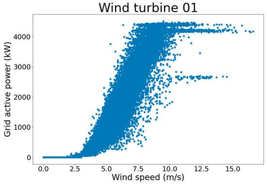
Figure 7. Wind power curve of wind turbine 01 in reality.

The power curve of the wind turbine is dynamic; it is not smooth due to the variations of factors, including the weather, air density, system controls, location and so on. The output wind power fluctuates according to the wind speeds at any given time. In this study, the coding language used was Python, and the training model was implemented using Keras 2.9 and Keras-TCN 3.4.4. In order to evaluate the performance of the proposed model, the paper used the Mean Square Error (MSE) function of Scikit-learn 1.1.1 and calculated the forecasting errors. All resulting figures of the proposed model were plotted by functions of Matplotlib 3.4.3. The parameters of the computer are Intel (R) Core (TM) i7-10700K CPU @3.8 GHz, Ram 64 GB.

4.1. Preprocessing Data

In this dataset, the meteorological factors include temperature, wind speed, and wind direction measured at 100 m. After collecting the data of 14 turbines from historical measurements, the dataset was resampled from 1 min to 30 min by aggregating with the mean function. The time step interval in this study is 30 min because of the resolution of the collected dataset. Since the length of time for the collected data is around four months (from April to July 2022), the historical time window is about three months. Although the length of time is short, it provides a good opportunity to propose a suitable training model with a limited amount of data. Moreover, when the historical time window is increased, a large amount of input data would increase the computation burden for constructing forecasting models.

This study aims to develop a new TCN approach for short-term wind power forecasting (30 min to 6 h ahead). Thus, the selected size of the historical time window with 30-min data resolution should be suitable for our short-term forecasts. Then, this study combined the data of all turbines and calculated the Pearson and Spearman correlation as follows:

As shown in Table 2, the wind direction needs to be excluded since it is weakly related to wind power. Next, the Orange software continues to remove its outliers by applying the Covariance Estimator algorithm. After removing outliers, the used dataset includes 30236 samples in total (14 wind turbines, the data resolution: 30 min). The wind power project’s total data divides into three parts. The training, testing and validation dataset includes respectively 21,165, 4535, and 4536 samples. The Pearson and Spearman correlation is calculated to demonstrate the effectiveness of the Covariance Estimator algorithm of the Orange software as follows:

Table 2. Pearson and Spearman correlation results of the collected dataset.

Pearson Correlation
	Wind speed	Wind direction	Ambient temperature	Grid active power
Wind speed	1	−0.034	−0.1644	0.9505
Wind direction	−0.034	1	−0.0202	−0.0253
Ambient temperature	−0.1644	−0.0202	1	−0.1553
Grid active power	0.9505	−0.0253	−0.1553	1
Spearman Correlation
	Wind speed	Wind direction	Ambient temperature	Grid active power
Wind speed	1	0.046	0.141	0.991
Wind direction	0.046	1	0.006	0.044
Ambient temperature	0.141	0.006	1	−0.141
Grid active power	0.991	0.044	−0.141	1

As shown in Table 3, it is noticeable that the grid active power has a strong relationship with the wind speed based on the PCC and SCC. The results approximate one, which means that there is a positive correlation between the two variables. While the Pearson correlation measures the strength of the linear relationship between them, the Spearman correlation measures the strength of a monotonic relationship. Besides, the SCC and PCC between the ambient temperature and grid active power are very close to zero. In other words, they are considered weak. However, when experimenting, we realized that the forecasting models in this study perform better with the input data, including wind speed, ambient temperature, and active power. The results are described in Section 4.3.

Table 3. Pearson and Spearman correlation results after removing outliers by applying the Covariance Estimator of Orange software.

Pearson Correlation
	Wind speed	Ambient temperature	Grid active power
Wind speed	1	−0.0002	0.9801
Ambient temperature	−0.0002	1	−0.018
Grid active power	0.9801	−0.018	1
Spearman Correlation
	Wind speed	Ambient temperature	Grid active power
Wind speed	1	0.032	0.995
Ambient temperature	0.032	1	0.024
Grid active power	0.995	0.024	1

4.2. Training Model

In this study, the time step interval is 30 min. These time steps are divided into six historical and six future steps. Figure 8 clarifies the training inputs and outputs of the prediction modeling.

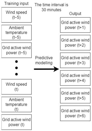
Figure 8. The relationship between training inputs and output of the prediction modeling.

Before training the model, the following parameters are configured: the batch size is set to 128, the maximum number of iterations is 500, and the dropout rate is 0.1. The overfitting problem is checked by investigating the learning curve of models.

Overfitting can appear on a learning curve if:

• The plot of training loss continues to decline with experience;
• The plot of validation loss falls to a point and begins to rise again.

Learning curves show a good fit if:

• The plot of training loss decreases to a stable point;
• The plot of validation loss decreases to a stable point and has a small gap with training loss.

The utilized algorithm for optimization is Adam Algorithm [31], and the loss function is the Mean Squared Error (MSE). Figure 9 shows the validation and training loss curves. As the number of iterations increases in Figure 9, the loss functions of S-TCN decrease. After around 400 epochs, they tend to be stable fast and have small fluctuations. Moreover, the gap between the training and validation loss curve after training is small, indicating that the proposed S-TCN method has strong generalization and no over-fitting.

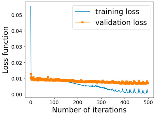
Figure 9. The training and loss validation curve of the model 5 stacks TCN.

To prevent overfitting problems, the model complexity can be adjusted, which includes the change of network structure (number of weights) or the change of network parameters (values of weights). Moreover, the dropout technique can also be used as a regularization technique that prevents the network from overfitting. It can modify the network automatically to prevent the network from overfitting by randomly dropping some neurons in the hidden layers during each iteration of model training.

4.3. Evaluating Model

In order to prove the efficiency of the proposed model, the other forecasting models that were widely used are also examined. These models include the Vanilla LSTM, Stacked LSTM (S-LSTM), Bidirectional LSTM (Bi-LSTM), Convolutional LSTM (Conv-LSTM) and conventional TCN models. Moreover, experiments with two, three, four, and five stacked layers of TCN are investigated. After training these models with the same training set, they are used to predict the wind power of the test set. This study investigated two cases of input data to demonstrate the importance of ambient temperature in wind power forecasting. First, the historical wind speed, ambient temperature, and power measurements are used as inputs for our forecasting models. Second, the input data excludes the ambient temperature. Table 4 and Table 5 demonstrate the evaluation metrics RMSE and MAE using different models for each forecasting time step and show the training time of each model.

Table 4. Performance and training time of different forecasting models with the input data, including the wind speed, ambient temperature and grid active power.

	RMSE (kW)
Model	Step t + 1	Step t + 2	Step t + 3	Step t + 4	Step t + 5	Step t + 6
Vanilla LSTM	239.13	313.69	351.64	385.56	420.74	457.28
S-LSTM	230.10	300.45	340.43	372.97	407.96	443.12
Bi-LSTM	216.98	290.92	335.90	367.77	398.10	432.34
Conv-LSTM	221.43	315.12	363.77	406.90	448.66	485.83
TCN	198.69	262.79	300.85	338.69	365.11	389.37
2 stacks TCN	200.12	259.8	259.80	319.50	342.29	365.14
3 stacks TCN	186.63	239.42	267.62	297.15	323.91	351.59
4 stacks TCN	189.53	239.82	271.28	300.1	325.11	347.73
5 stacks TCN	196.43	251.23	277.53	301.49	331.01	354.39
	MAE (kW)
Model	Step t +1	Step t + 2	Step t + 3	Step t + 4	Step t + 5	Step t + 6
Vanilla LSTM	168.27	222.11	248.73	274.13	300.29	327.31
S-LSTM	158.65	210.28	236.76	261.94	284.38	312.16
Bi-LSTM	150.07	202.44	231.44	252.78	272.47	294.47
Conv-LSTM	149.21	219.42	254.27	282.90	308.58	330.68
TCN	134.63	176.46	197.33	218.58	232.61	249.01
2 stacks TCN	132.75	174.32	192.33	204.43	219.27	235.75
3 stacks TCN	123.53	156.36	171.16	185.06	198.6	215.68
4 stacks TCN	123.12	154.99	172.39	186.31	198.58	211.47
5 stacks TCN	131.68	164.11	178.49	192.73	209.76	222.75
	Training time
Model
Vanilla LSTM	2 min and 30 s
S-LSTM	3 min and 45 s
Bi-LSTM	16 min and 10 s
Conv-LSTM	13 min and 20 s
TCN	10 min and 40 s
2 stacks TCN	20 min and 20 s
3 stacks TCN	41 min and 35 s
4 stacks TCN	50 min and 33 s
5 stacks TCN	66 min and 51 s

Table 5. Performance and training time of different forecasting models with the input data, including the wind speed and grid active power.

	RMSE (kW)
Model	Step t + 1	Step t + 2	Step t + 3	Step t + 4	Step t + 5	Step t + 6
Vanilla LSTM	238.28	336.22	390.7	437.32	481.75	518.46
S-LSTM	234.25	324.57	376.08	416.16	453.47	486.04
Bi-LSTM	257.09	348.09	400.9	443.29	486.69	521.85
Conv-LSTM	234.2	330.77	386.76	434.25	478.17	513.47
TCN	234.34	327.62	377.79	425.28	467.37	504.68
2 stacks TCN	221.48	285.97	331.1	368.16	398.34	419.07
3 stacks TCN	213.84	288.65	341.31	378.86	410.57	428.7
4 stacks TCN	215.9	280.79	328.19	363.37	390.74	419.62
5 stacks TCN	218.27	292.56	338.91	373.72	404.714	433.58
	MAE (kW)
Model	Step t + 1	Step t + 2	Step t + 3	Step t + 4	Step t + 5	Step t + 6
Vanilla LSTM	160.32	232.6	273	309.94	343.44	369.85
S-LSTM	163.7	227.52	263.5	293.47	321.43	345.32
Bi-LSTM	173.33	240.49	277.01	307.75	337.82	362.15
Conv-LSTM	155.08	225.76	264.57	297.9	329.15	355.27
TCN	155.14	224.21	260.55	293.43	326.79	351.98
2 stacks TCN	140.24	187.75	212.92	235.11	252	266.84
3 stacks TCN	139.25	184.08	215.55	236.6	255.44	269.03
4 stacks TCN	138.41	181.28	208.02	226.07	242.43	261.53
5 stacks TCN	142.09	189.66	213.35	232.32	248.89	266.71
	Training time
Model
Vanilla LSTM	1 min and 10 s
S-LSTM	3 min and 5 s
Bi-LSTM	15 min and 35 s
Conv-LSTM	16 min and 17 s
TCN	9 min and 8 s
2 stacks TCN	18 min and 11 s
3 stacks TCN	40 min and 55 s
4 stacks TCN	50 min and 35 s
5 stacks TCN	65 min and 4 s

From the above tables, it is noticeable that the performance of all models in Table 5 is worse than that in Table 4. In other words, the models perform better if the input data include wind speed, ambient temperature, and active power.

The dataset was collected from the Tan Thuan wind power plant located at Ca Mau from April to July 2022. Ca Mau is a city in southern Vietnam and has a tropical monsoon climate with a lengthy wet season and a relatively dry season. Thus, the prevailing wind follows the seasonal mode. The wet season lasts from April to December. The dry season lasts from January to March. The average temperature is high, but it rises noticeably in April or May, which signals the upcoming rainy or monsoon season. The correlation between wind speed and ambient temperature may be affected by seasonal characteristics. Indeed, the results of this study demonstrate the importance of ambient temperature in wind power forecasting, which helps improve the performance of the forecasting model.

From Table 4, it can be seen that the forecasting accuracy using the three or four stacked-layer TCN models is slightly different but lower than the predecessor models such as LSTM, Stacked LSTM or traditional TCN, revealing that the S-TCN models are appropriate for short-term wind power forecasts because they can connect the complicated relationship between meteorological variables and wind power generation. The training duration of the predecessor models took less time than the TCN and S-TCN models. Obviously, as a higher number of stacks of TCN is used, a longer computation time is required. It is no doubt that training a deep learning model requires a significant amount of computation time according to model complexity. However, the required computation time for training a lower-stack TCN model (i.e., three-stack TCN) is still acceptable in real industrial applications. Thus, this study suggests selecting three to four stacks for the S-TCN structure. The developed S-TCN represents longer time scales up to an entire sequence by stacking causal dilated convolutions and residual connections to create much larger receptive fields. In terms of multi-step ahead forecasting, Figure 10 shows the actual and forecasted values by the three stacked layers of the TCN model for 50 samples at each time step of the test set.

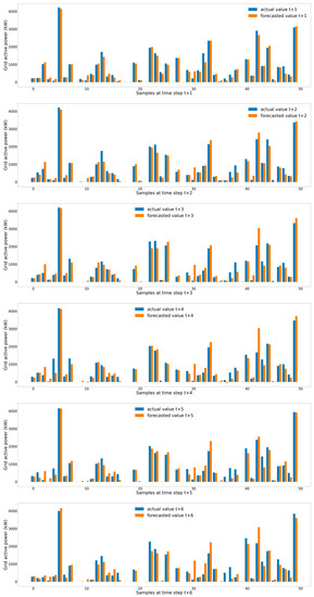
Figure 10. Actual and forecasted values at each time step of 50 samples in the test set.

5. Conclusions

There are the following conclusions after training and evaluating the proposed S-TCN model:

• S-TCN has fast convergence. The whole training process is stable, and the gap between the training and validation loss curve is very small, indicating that S-TCN has the characteristics of strong generalization;
• The RMSE and MAE results using the S-TCN model are the smallest compared to the other models, which shows that the proposed S-TCN is very suitable for short-term multi-step wind power predictions.

In summary, this study provides a novel S-TCN structure for multi-step wind power forecasting. The proposed S-TCN exhibits a longer memory than recurrent architectures with the same capacity, thanks to its dilated convolution. Additionally, the causal convolution is realized by padding to prevent information leakage effectively. These advantages help the receptive field size become more flexible and achieve exponential. Moreover, the residual connection of the S-TCN model can reduce prediction errors. Besides, during the training model, S-TCN has the capacity for strong generalization, which means that it can prevent vanishing gradients through a stable training process. An increase in TCN layers number is able to help extract temporal features more precisely; however, it prolongs the training process. This study only considered one Vietnam wind farm as our demonstration site for evaluating the proposed forecasting model. Additionally, the collected data are limited. In the future, this study will utilize more data from other wind farms to confirm the robustness of the proposed method. Transfer learning will be carefully considered to increase the training efficiency and accuracy of the S-TCN network when dealing with other datasets.

References

- Wang, Y.; Zou, R.; Liu, F.; Zhang, L.; Liu, Q. A Review of Wind Speed and Wind Power Forecasting with Deep Neural Networks. Appl. Energy 2021, 304, 117766. [Google Scholar] [CrossRef]
- Mao, Y.; Shaoshuai, W. A Review of Wind Power Forecasting & Prediction. In Proceedings of the 2016 International Conference on Probabilistic Methods Applied to Power Systems, PMAPS 2016, Beijing, China, 16–20 October 2016. [Google Scholar] [CrossRef]
- Zhao, W.; Wei, Y.M.; Su, Z. One Day Ahead Wind Speed Forecasting: A Resampling-Based Approach. Appl. Energy 2016, 178, 886–901. [Google Scholar] [CrossRef]
- Cao, Y.; Gui, L. Multi-Step Wind Power Forecasting Model Using LSTM Networks, Similar Time Series and LightGBM. In Proceedings of the 2018 5th International Conference on Systems and Informatics, ICSAI 2018, Nanjing, China, 10–12 November 2018; IEEE: Piscataway, NJ, USA, 2019; pp. 192–197. [Google Scholar] [CrossRef]
- Ait Maatallah, O.; Achuthan, A.; Janoyan, K.; Marzocca, P. Recursive Wind Speed Forecasting Based on Hammerstein Auto-Regressive Model. Appl. Energy 2015, 145, 191–197. [Google Scholar] [CrossRef]
- Kavasseri, R.G.; Seetharaman, K. Day-Ahead Wind Speed Forecasting Using f-ARIMA Models. Renew. Energy 2009, 34, 1388–1393. [Google Scholar] [CrossRef]
- Han, Q.; Meng, F.; Hu, T.; Chu, F. Non-Parametric Hybrid Models for Wind Speed Forecasting. Energy Convers. Manag. 2017, 148, 554–568. [Google Scholar] [CrossRef]
- Yunus, K.; Thiringer, T.; Chen, P. ARIMA-Based Frequency-Decomposed Modeling of Wind Speed Time Series. IEEE Trans. Power Syst. 2016, 31, 2546–2556. [Google Scholar] [CrossRef]
- Shi, Z.; Liang, H.; Dinavahi, V. Direct Interval Forecast of Uncertain Wind Power Based on Recurrent Neural Networks. IEEE Trans. Sustain. Energy 2018, 9, 1177–1187. [Google Scholar] [CrossRef]
- Duan, J.; Zuo, H.; Bai, Y.; Duan, J.; Chang, M.; Chen, B. Short-Term Wind Speed Forecasting Using Recurrent Neural Networks with Error Correction. Energy 2021, 217, 119397. [Google Scholar] [CrossRef]
- Wang, Y.; Liao, W.; Chang, Y. Gated Recurrent Unit Network-Based Short-Term Photovoltaic Forecasting. Energies 2018, 11, 2163. [Google Scholar] [CrossRef]
- Phan, Q.-T.; Wu, Y.-K.; Phan, Q.-D.; Lo, H.-Y. A Novel Forecasting Model for Solar Power Generation by a Deep Learning Framework with Data Preprocessing and Postprocessing. IEEE Trans. Ind. Appl. 2023, 59, 220–231. [Google Scholar] [CrossRef]
- Kamal, I.M.; Wahid, N.A.; Bae, H. Gene Expression Prediction Using Stacked Temporal Convolutional Network. In Proceedings of the 2020 IEEE International Conference on Big Data and Smart Computing, BigComp 2020, Busan, Republic of Korea, 19–22 February 2020; pp. 402–405. [Google Scholar] [CrossRef]
- Phan, Q.-T.; Wu, Y.-K.; Phan, Q.-D. A Comparative Analysis of XGBoost and Temporal Convolutional Network Models for Wind Power Forecasting. In Proceedings of the 2020 International Symposium on Computer, Consumer and Control (IS3C), Taichung City, Taiwan, 13–16 November 2020; IEEE: Piscataway, NJ, USA, 2020; pp. 416–419. [Google Scholar]
- Zhu, R.; Liao, W.; Wang, Y. Short-Term Prediction for Wind Power Based on Temporal Convolutional Network. Energy Rep. 2020, 6, 424–429. [Google Scholar] [CrossRef]
- Huang, B.; Liang, Y.; Qiu, X. Wind Power Forecasting Using Attention-Based Recurrent Neural Networks: A Comparative Study. IEEE Access 2021, 9, 40432–40444. [Google Scholar] [CrossRef]
- Aslam, M.; Kim, J.S.; Jung, J. Multi-Step Ahead Wind Power Forecasting Based on Dual-Attention Mechanism. Energy Rep. 2023, 9, 239–251. [Google Scholar] [CrossRef]
- Zhu, J.; Su, L.; Li, Y. Wind Power Forecasting Based on New Hybrid Model with TCN Residual Modification. Energy AI 2022, 10, 100199. [Google Scholar] [CrossRef]
- Liu, Q.; Che, X.; Bie, M. R-STAN: Residual Spatial-Temporal Attention Network for Action Recognition. IEEE Access 2019, 7, 82246–82255. [Google Scholar] [CrossRef]
- He, Y.; Zhao, J. Temporal Convolutional Networks for Anomaly Detection in Time Series. J. Phys. Conf. Ser. 2019, 1213, 042050. [Google Scholar] [CrossRef]
- Yu, F.; Koltun, V. Multi-Scale Context Aggregation by Dilated Convolutions. In Proceedings of the 4th International Conference on Learning Representations, ICLR 2016—Conference Track Proceedings, San Juan, Puerto Rico, 2–4 May 2016. [Google Scholar] [CrossRef]
- He, K.; Zhang, X.; Ren, S.; Sun, J. Deep Residual Learning for Image Recognition. In Proceedings of the IEEE Computer Society Conference on Computer Vision and Pattern Recognition, Boston, MA, USA, 7–12 June 2015; pp. 770–778. [Google Scholar] [CrossRef]
- Hara, K.; Saito, D.; Shouno, H. Analysis of Function of Rectified Linear Unit Used in Deep Learning. In Proceedings of the International Joint Conference on Neural Networks, Killarney, Ireland, 12–17 July 2015. [Google Scholar] [CrossRef]
- Wang, Y.; Chen, J.; Chen, X.; Zeng, X.; Kong, Y.; Sun, S.; Guo, Y.; Liu, Y. Short-Term Load Forecasting for Industrial Customers Based on TCN-LightGBM. IEEE Trans. Power Syst. 2021, 36, 1984–1997. [Google Scholar] [CrossRef]
- Phan, Q.-T.; Wu, Y.-K.; Phan, Q.-D.; Lo, H.-Y. A Novel Forecasting Model for Solar Power Generation by a Deep Learning Framework with Data Preprocessing and Postprocessing. In Proceedings of the Conference Record—Industrial and Commercial Power Systems Technical Conference, Las Vegas, NV, USA, 17–31 May 2022. [Google Scholar]
- Sadeghi, B. Chatterjee Correlation Coefficient: A Robust Alternative for Classic Correlation Methods in Geochemical Studies—(Including “TripleCpy” Python Package). Ore. Geol. Rev. 2022, 146, 104954. [Google Scholar] [CrossRef]
- Zwilling, C.E.; Wang, M.Y. Covariance Based Outlier Detection with Feature Selection. In Proceedings of the 2016 38th Annual International Conference of the IEEE Engineering in Medicine and Biology Society (EMBC), Orlando, FL, USA, 16–20 August 2016; pp. 2606–2609. [Google Scholar] [CrossRef]
- Outliers—Orange Visual Programming 3 Documentation. Available online: https://orange3.readthedocs.io/projects/orange-visual-programming/en/latest/widgets/data/outliers.html (accessed on 23 February 2023).
- Ge, L.; Liao, W.; Wang, S.; Bak-Jensen, B.; Pillai, J.R. Modeling Daily Load Profiles of Distribution Network for Scenario Generation Using Flow-Based Generative Network. IEEE Access 2020, 8, 77587–77597. [Google Scholar] [CrossRef]
- Mehdiyev, N.; Enke, D.; Fettke, P.; Loos, P. Evaluating Forecasting Methods by Considering Different Accuracy Measures. Procedia Comput. Sci. 2016, 95, 264–271. [Google Scholar] [CrossRef]
- Kingma, D.P.; Ba, J.L. Adam: A Method for Stochastic Optimization. In Proceedings of the 3rd International Conference on Learning Representations, ICLR 2015—Conference Track Proceedings, San Diego, CA, USA, 7–9 May 2015. [Google Scholar] [CrossRef]
Disclaimer/Publisher’s Note: The statements, opinions and data contained in all publications are solely those of the individual author(s) and contributor(s) and not of MDPI and/or the editor(s). MDPI and/or the editor(s) disclaim responsibility for any injury to people or property resulting from any ideas, methods, instructions or products referred to in the content. |
© 2023 by the authors. Licensee MDPI, Basel, Switzerland. This article is an open access article distributed under the terms and conditions of the Creative Commons Attribution (CC BY) license (https://creativecommons.org/licenses/by/4.0/).