Optimal Neutral Grounding in Bipolar DC Networks with Asymmetric Loading: A Recursive Mixed-Integer Quadratic Formulation

Abstract

This paper presents a novel approach to tackle the problem of optimal neutral wire grounding in bipolar DC networks including asymmetric loading, which naturally involves mixed-integer nonlinear programming (MINLP) and is challenging to solve. This MINLP model is transformed into a recursive mixed-integer quadratic (MIQ) model by linearizing the hyperbolic relation between voltage and powers in constant power terminals. A recursive algorithm is implemented to eliminate the possible errors generated by linearization. The proposed recursive MIQ model is assessed in two bipolar DC systems and compared against three solvers of the GAMS software. The results obtained validate the performance of the proposed MIQ model, which finds the global optimum of the model while reducing power losses for bipolar DC systems with 21, 33, and 85 buses by 4.08%, 2.75%, and 7.40%, respectively, when three nodes connected to the ground are considered. Furthermore, the model exhibits a superior performance when compared to the GAMS solvers. The impact of grounding the neutral wire in bipolar DC networks is also studied by varying the number of available nodes to be grounded. The results show that the reduction in power losses is imperceptible after grounding the third node for the three bipolar DC systems under study.

1. Introduction

1.1. General Context

Electrical distribution networks are continuously being transformed with the advances made in electronic power conversion, distributed energy resources, and hybrid distribution technologies [1]. These grids have transitioned from passive distribution to active distribution configurations, with the main advantage of self-managing all of their distributed energy resources from an optimization perspective, with the aim to maximize the quality of the energy service [2,3]. Regarding grid distribution technologies, distribution networks operating with direct current (DC) technologies have recently gained more attention, given their advantages over conventional alternating current (AC) distribution technologies [4,5,6]. These advantages include the following:

i.

Reduced energy losses due to resistive effects in cables operated with DC are lower than those in cables operated with AC due to the skin effect [7]. Additionally, these energy losses are also reduced because, in DC networks, no reactance effects are considered. This implies that the voltage droops in the lines are lower, resulting in reduced current magnitudes for these branches. This reduction is directly linked to the power loss level [8].

ii.

DC networks are easily controllable, as the only variable of interest is the voltage supplied at the substation bus, which is a real and constant variable. The main advantage is that no frequency issues are considered since this variable does not exist in DC technology [9].

iii.

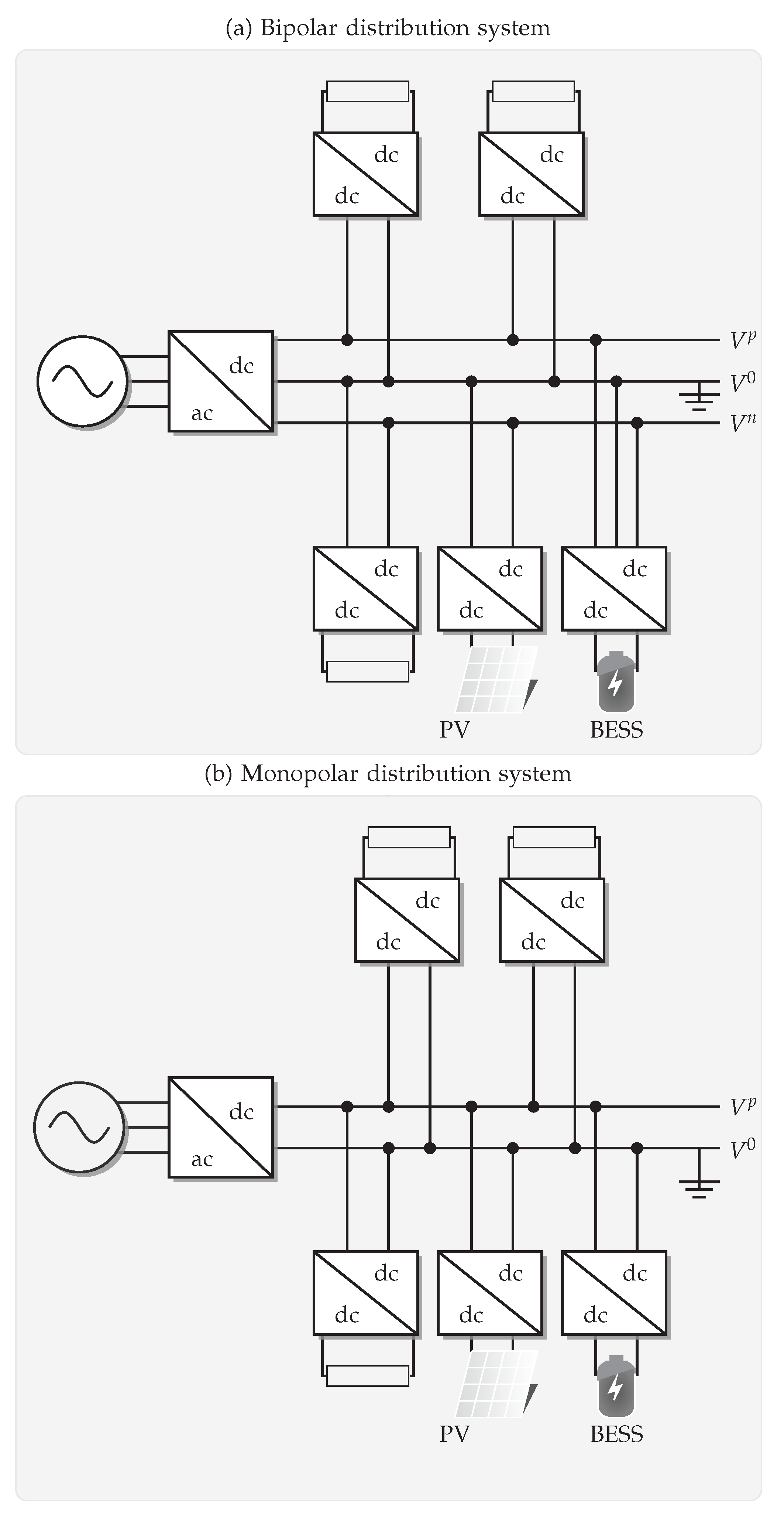
DC technology is the natural choice for operating batteries, photovoltaic (PV) sources, fuel cells, supercapacitors, and superconductor energy storage systems. This implies that integrating these devices in DC grids requires fewer power conversion stages, which can reduce the expected investment costs and increase the reliability of the entire grid by reducing the number of cascade devices (i.e., DC to AC conversion stages) [10,11].

Considering the advantages of DC distribution technologies, it is also worth considering the possible grid configurations applicable to DC distribution grids, i.e., monopolar or bipolar [12,13,14]. Figure 1 depicts the two possible DC grid configurations.

These grid topologies applicable to DC networks, as depicted in Figure 1, reveal that: (i) bipolar DC networks can support more than two times the expected power consumption, as they have two poles fed with $\pm V_{DC}$ [15]; (ii) bipolar DC networks can contain special loads operated with two times the voltage applied to one of the poles (i.e., $2V_{DC}$), which is not possible with monopolar DC configurations [16]; and (iii), the expected costs of a bipolar DC network include an additional wire (neutral wire) and a bipolar DC converter, which can increase the construction costs by only about $33.34\%$ concerning a conventional monopolar DC network [17].

1.2. Motivation

Even though the advantages of bipolar DC grids are evident when compared with monopolar DC systems, using two poles implies that these grids will operate under unbalanced conditions, as constant power loads in the positive and negative poles concerning the neutral wire are generally not balanced [18]. This characteristic implies higher power losses than those associated with an ideal operation case [19,20]. In addition, the neutral wire can be considered with two typical connections: solidly grounded in all network nodes or floating. Nevertheless, solid grounding constitutes the ideal operation case, given that the voltage profile will be better than the scenario involving a floating neutral wire, and the energy losses will be lower. This operation scenario is economically infeasible due to the high costs associated with the implementation of neutral grounding, especially in bipolar DC distribution networks with hundreds of nodes. Additionally, bipolar DC networks with asymmetric loads and multiple nodes may entail a complicated operation. All the challenges above have motivated this research to propose an efficient optimization model to determine the best set of nodes to implement neutral grounding connections, in order to minimize the expected grid power losses and improve the voltage profile.

1.3. Literature Review

Bipolar DC networks for distribution network applications have gained significant attention in the last ten years. Multiple authors have focused on proposing efficient methodologies for solving the power flow, the optimal power flow, and the load balancing problems, among others, particularly under steady-state operating conditions. Some of these works are discussed below.

The authors of [18] presented a generic solution methodology for the power flow problem in bipolar asymmetric DC networks through the Newton-Raphson formulation. The power flow formulation is based on the current injection method. Six different node types were defined as a function of the grounding scenario and the voltage control method in the generation sources. The effectiveness of the Newton-Raphson method in dealing with the power flow problem in bipolar DC networks was validated via the PSCAD/EMTDC software.

In [21], the power flow problem in distribution networks was considered to have a bipolar structure, and asymmetric loading was addressed by applying the successive approximations method. Numerical results in the 4- and 21-node grids demonstrate the effectiveness of this derivative-free approach, proving that it is equivalent to the classical backward/forward power flow approach when extended to unbalanced bipolar DC grids.

The works by [22,23] presented the solution to the optimal power flow problem in bipolar asymmetric distribution networks using a bilinear formulation based on the current injection method. The main goal of these works was reducing the nodal marginal prices caused by asymmetric loading, as the congestion in the distribution lines, given that load imbalance implies different values between the positive and negative poles downstream of the substation bus.

The research by [19,24] presented two convex approximations to solve the optimal power flow problem in bipolar DC networks while considering asymmetric loading and neutral floating operating conditions. The first approach was based on the recursive linearization procedure applied to the hyperbolic constraints regarding constant power loads using Taylor’s series expansion. The second approach involved the representation of these hyperbolic constraints using a cone representation of the product between two positive variables. Numerical results in the 21- and 85-bus grids demonstrated the effectiveness and robustness of the convex models when compared to the sine cosine algorithm, the black hole optimizer, and the Chu and Beasley genetic algorithm.

The study by [25] addressed the optimal power flow problem in bipolar DC networks with asymmetric loading through a quadratic convex approximation based on the current injection formulation. Three objective functions were considered to define the optimal generation outputs of the dispersed generation sources, i.e., minimizing generation costs and energy losses and improving voltage imbalance. Numerical results in the 33- and 85-bus networks demonstrated the effectiveness of this convex formulation in four simulation scenarios.

The authors of [16] presented a multi-objective formulation to solve the optimal load balancing problem in asymmetric bipolar DC networks via a mixed-integer formulation. The objective functions under analysis corresponded to voltage load balancing in the positive and negative poles and the reduction of the expected power losses. Even though this optimization model is a mixed-integer convex formulation, the main problem with this research is that the authors only considered linear loads, which implies that the nonlinearities introduced by the constant power terminals were neglected.

In [17], the optimal pole swapping problem in bipolar DC networks with asymmetric loading was solved while considering multiple unbalanced load terminals. The main contribution of this research was the hybridization of the sine cosine algorithm, the black hole optimizer, and the Chu and Beasley genetic algorithm with the triangular-based power flow problem within a master-slave strategy in order to select the best set of load interchanges. This, with the aim to minimize the total grid power losses. Numerical validations were carried out in the 21- and 85-bus grids, where the Chu and Beasley genetic algorithm reported the best numerical performance.

The above literature review allowed noting the relevance of bipolar DC networks due to their advantages in comparison with monopolar DC networks or AC conventional systems. Nevertheless, most of the recent developments are focused on solving the power flow, the optimal power flow, and the load balancing (or pole swapping) problems. However, no contributions regarding the efficient solid grounding of neutral wires were found. This represents a clear gap in bipolar grid analysis, which this work attempts to fill.

1.4. Contributions and Scope

Considering the literature review and challenges and opportunities in proposing new methodologies for analyzing bipolar DC networks, this paper makes the following contributions:

i.

A mixed-integer convex model is proposed to represent the optimal selection of nodes to be solidly grounded in order to minimize the total grid power losses.

ii.

The convex approximation model uses the first Taylor term to linearize the nonlinear relation between powers and voltages in the constant power demands.

iii.

A recursive solution methodology is presented to reduce/eliminate the error introduced by the linearization approach. This methodology is based on Taylor’s series expansion, which updates the voltages in all of the network poles at each iteration until the desired convergence error is reached.

iv.

Numerical results in three test systems demonstrate the performance and effect of the model in reducing the grid power losses.

Numerical results in bipolar asymmetric networks composed of 21 and 33 nodes demonstrate the effectiveness and robustness of this recursive mixed-integer convex solution methodology in comparison with the solution of the exact mixed-integer nonlinear programming (MINLP) model, which is obtained via the different solvers available in the general algebraic modeling system (GAMS) software. On the other hand, it is essential to mention that, in the scope of this research, all load nodes are modeled as constant power loads, as this is the most critical modeling, given the hyperbolic nonlinearities introduced by these loads regarding voltage profiles.

It is worth mentioning that this is the first time that the problem regarding optimal neutral grounding has been addressed in the scientific literature. Therefore, comparisons are only made with different MINLP solvers available in the GAMS software, which implies that the main contribution in this research is the demonstration that, with a reduced number of nodes for the implementation of solid neutral grounding (less than 15% of the total grid nodes), it is possible to have near-ideal power losses when all nodes are assumed to be solidly grounded.

1.5. Document Structure

The remainder of this document is organized as follows. Section 2 presents the exact MINLP formulation regarding optimal neutral grounding in bipolar DC grids with asymmetric loading. The main complication of this optimization model lies in the hyperbolic constraints introduced by the constant power loads, which transform the nonlinear programming component of the optimization model into a non-convex set of constraints. Section 3 describes the proposed solution methodology, which is based on the linearization of the hyperbolic constraints via Taylor’s series expansion. To reduce/eliminate the error introduced by Taylor’s linearization, a recursive solution approach is adopted until the error between voltages is minimized in all poles in two consecutive iterations. Section 4 shows the analyzed test feeders’ main characteristics, i.e., the DC bipolar asymmetric versions of the 21- and 33-node grids. Section 5 describes the main numerical achievements, comparisons, and discussions regarding the proposed mixed-integer quadratic approximation vs. the solution of the exact MINLP model by means of different solvers available in GAMS. Finally, Section 6 lists the main concluding remarks derived from this work, as well as some future research approaches.

2. Optimal Neutral Grounding Model

The effective selection of optimal nodes for a grounding strategy to minimize power losses in bipolar DC grids can be modeled as a mixed-integer nonlinear programming (MINLP) problem [25]. The solution to this problem requires identifying the best set of nodes to implement a solid grounding strategy on the neutral wire. This allows the system to operate efficiently and minimizes the total power losses. The MINLP model is presented below.

2.1. Objective Function

The objective function of the studied problem involves the reduction of the total power losses ($p_{\mathrm{loss}}$) of the bipolar DC network, i.e., all of the electrical energy dissipated in heat by the resistive effects of the system lines [17]. The objective function takes the following form:

$$\begin{array}{c}min{p}_{\mathrm{loss}}=\sum _{r\in \mathcal{P}}\sum _{j\in \mathcal{N}}{v}_j^r\left(\sum _{s\in \mathcal{P}}\sum _{kin\mathcal{N}}{g_{jk}}^{rs}{v}_k^s\right),\end{array}$$

(1)

where $v_j^r$ and $v_k^s$ are the voltage values at node j for the r-th pole and at node k for the s-th pole, respectively; $g_{jk}^{rs}$ is the value of the conductance matrix associated with nodes j and k, which is between poles r and s; $\mathcal{P}\in \left\{p,o,n\right\}$ denotes the set of poles (e.g., positive, neutral, and negative) in the bipolar DC network; $\mathcal{N}$ represents to the set of nodes in the bipolar DC network; r and s are pole-related superscripts, while j and k are node-related subscripts.

It is essential to mention that, in order to calculate the total power losses ($p_{\mathrm{loss}}$) in the objective function (1), when there is a mutual coupling conductance between two poles, the value of $g_{jk}^{rs}$ will be different from zero if $j=k$ and $r\ne s$; otherwise, $g_{jk}^{rs}$ will always be zero if $r\ne s$.

2.2. Set of Constraints

The set of constraints for the optimal neutral grounding model is related to the physical operation and regulation characteristics of bipolar DC networks. This model is composed of the current balance at each pole and each network node, the limits of the power generators, the power capacity of the transmission lines, the maximum and minimum voltage levels at each node, and the decision to ground the neutral wire or not.

2.2.1. Current Balance Equation

The current balances at each node and pole of the bipolar network are obtained by applying Kirchhoff’s first law:

$$\begin{array}{c}\hfill i_{gk}^p-i_{dk}^p-i_{dk}^{p-n}=\sum _{r\in \mathcal{P}}\sum _{j\in \mathcal{N}}{g}_{jk}^{pr}{v}_k^r,\left\{\forall k\in \mathcal{N}\right\}\end{array}$$

(2)

$$\begin{array}{c}\hfill i_{gk}^o-i_{dk}^o-i_{dk}^{\mathrm{gr}}=\sum _{r\in \mathcal{P}}\sum _{j\in \mathcal{N}}{g}_{jk}^{or}{v}_k^r,\left\{\forall k\in \mathcal{N}\right\}\end{array}$$

(3)

$$\begin{array}{c}\hfill i_{gk}^n-i_{dk}^n+i_{dk}^{p-n}=\sum _{r\in \mathcal{P}}\sum _{j\in \mathcal{N}}{g}_{jk}^{nr}{v}_k^r,\left\{\forall k\in \mathcal{N}\right\}\end{array}$$

(4)

where $i_{gk}^p$, $i_{gk}^o$, and $i_{gk}^n$ are currents injected by the generator into node k for each pole (positive p, neutral o, and negative n); $i_{dk}^p$, $i_{dk}^o$, and $i_{dk}^n$ are currents absorbed by the loads at node k for each pole; $i_{dk}^{p-n}$ is the current absorbed by the load at node k connected between the positive and negative poles; and $i_{dk}^{\mathrm{gr}}$ is the total current drained to the ground at node k.

2.2.2. Current Demand Formulation

The currents absorbed by the loads must be modeled as a function of the constant power load, which can be connected between the positive and neutral poles or the negative and neutral poles (which is known as a monopolar load), as well as between the positive and negative poles (bipolar load). This model generates a hyperbolic relation between voltage and powers, as follows:

$$\begin{array}{c}\hfill i_{dk}^{p-n}=\frac{p_{dk}^{p-n}}{v_k^p-v_k^n},\left\{\forall k\in \mathcal{N}\right\}\end{array}$$

(5)

$$\begin{array}{c}\hfill i_{dk}^p=\frac{p_{dk}^p}{v_k^p-v_k^o},\left\{\forall k\in \mathcal{N}\right\}\end{array}$$

(6)

$$\begin{array}{c}\hfill i_{dk}^n=\frac{p_{dk}^n}{v_k^n-v_k^o},\left\{\forall k\in \mathcal{N}\right\}\end{array}$$

(7)

$$\begin{array}{c}\hfill i_{dk}^o=-i_{dk}^p-i_{dk}^n,\left\{\forall k\in \mathcal{N}\right\}\end{array}$$

(8)

where $p_{dk}^p$ and $p_{dk}^n$ are the monopolar constant powers demanded by node k at poles p and n concerning the neutral pole, respectively; and $p_{dk}^{p-n}$ is the bipolar constant power demanded at node k connected between the positive and negative poles.

2.2.3. Operating Limits

The capacity limits of the generator bound its current injection as follows:

$$\begin{array}{c}\hfill i_{gk}^{p,min}\le i_{gk}^p\le i_{gk}^{p,max},\left\{\forall k\in \mathcal{N}\right\}\end{array}$$

(9)

$$\begin{array}{c}\hfill i_{gk}^{o,min}\le i_{gk}^o\le i_{gk}^{o,max},\left\{\forall k\in \mathcal{N}\right\}\end{array}$$

(10)

$$\begin{array}{c}\hfill i_{gk}^{n,min}\le i_{gk}^n\le i_{gk}^{n,max},\left\{\forall k\in \mathcal{N}\right\}\end{array}$$

(11)

where $i_{gk}^{p,min}$, $i_{gk}^{o,min}$, and $i_{gk}^{n,min}$ are the minimum currents that can be injected by the generator connected to node k the for positive, neutral, and negative poles, respectively; while $i_{gk}^{p,max}$, $i_{gk}^{o,max}$, and $i_{gk}^{n,max}$ are the maximum currents that can be injected by the generator connected to node k for the positive, neutral, and negative poles, respectively.

The voltage values must be bounded between minimum and maximum values for the satisfactory operation of a bipolar DC grid:

$$\begin{array}{}\mathrm{(12)}& \hfill v^{p,min}\le v_k^p\le v^{p,max},\left\{\forall k\in \mathcal{N}\right\}\mathrm{(13)}& \hfill v^{n,min}\le v_k^n\le v^{n,max},\left\{\forall k\in \mathcal{N}\right\}\mathrm{(14)}& \hfill {\left[\begin{array}{ccc}{v}_j^p& v_j^o& v_j^n\end{array}\right]}^{\top }={\left[\begin{array}{ccc}1& 0& -1\end{array}\right]}^{\top }{v}_{\mathrm{nom}},\left\{j=\mathrm{slack}\right\},\end{array}$$

where $v^{p,min}$ and $v^{p,max}$ are the maximum and minimum voltage allowed in the grid, respectively; and $v_j^p,v_j^o$, and $v_j^n$ are the voltages regulated by the generator connected to node j.

2.2.4. Grounding of the Neutral Wire

Representing a neutral ground connection requires a binary variable in order to be able to select which nodes are grounded and which are not. In addition, it must also be ensured that the pole voltage of the grounded node is zero. The following two inequalities are proposed in order to mathematically represent these constraints:

$$\begin{array}{}\mathrm{(15)}& \hfill -z_{k}M\le i_{dk}^{\mathrm{gr}}\le z_{k}M,\left\{\forall k\in \mathcal{N}\right\}\mathrm{(16)}& \hfill -\left(1-z_k\right)M\le v_k^o\le \left(1-z_k\right)M,\left\{\forall k\in \mathcal{N}\right\}\end{array}$$

where $z_k\in \left\{0,1\right\}$ denotes the binary variable that determines the grounding or not of the neutral wire at node k, and $M>0$ is a positive parameter known as the big-M number.

Note that inequality (15) represents the minimum and maximum current flowing through the neutral wire. In contrast, inequality (16) is a box constraint that limits the minimum and maximum voltage in the neutral pole.

Remark 1.

The mathematical model described from (1) to (16) is a non-convex MINLP model whose solution is rather problematic. Its global optimum is not guaranteed due to the hyperbolic relations between voltages and powers in (5)–(7). Therefore, with the purpose of reaching the global optimum, a recursive quadratic approximation is performed, which convexifies the set of Equations (5)–(7) using an equivalent linear approximation, as presented in the next section.

3. Recursive Quadratic Approximation for the Optimal Neutral Grounding

This section shows the transformation of the non-convex MINLP model presented in (1)–(16) into a convex approximation using the linearization presented in [19]. Now, the nonlinear and non-convex equations of the exact MINPL model are analyzed.

3.1. Objective Function Analysis

The objective function (1) is a quadratic function since there is a product between voltages to compute the power losses of the bipolar DC network. As a quadratic function, it is easy to determine whether the objective function is convex. Therefore, the objective function (1) can be rewritten as follows:

$$\begin{array}{c}\hfill p_{\mathrm{loss}}=x^{\top }Gx,\end{array}$$

(17)

where $x\in R^{3n}$ is a voltage vector, and $G\in R^{3nn}$ is the conductance matrix that contains the bipolar DC grid topology.

The quadratic function (17) is a convex function if and only if G is symmetric and positive semi-definite, which means that $G=G^{\top }⪰0$ and satisfies

$$\begin{array}{c}\hfill x^{\top }Gx\ge 0\forall x\in R^{3n}.\end{array}$$

(18)

The general demonstration of a quadratic function defined in (18) can be consulted in [26,27].

3.2. Linear Approximation Applied to Constant Power Loads

An auxiliary function $f\left(w,y\right)$ is invoked to linearize each node’s hyperbolic relation between voltage and power:

$$\begin{array}{c}\hfill f\left(w,y\right)=\frac{1}{w-y},\end{array}$$

(19)

which is approximated to a linear function using the first term of Taylor’s series expansion in two variables, as follows:

$$\begin{array}{c}\hfill \begin{array}{c}\hfill f\left(w,y\right)\approx f\left(w_0,y_0\right)+{\nabla }_{w}f\left(w_0,y_0\right)\left(w-w_0\right)+{\nabla }_{y}f\left(w_0,y_0\right)\left(y-y_0\right),\end{array}\end{array}$$

(20)

where $\left(w_0,y_0\right)$ denotes the linearization point, while ${\nabla }_{w}f\left(w_0,y_0\right)$ and ${\nabla }_{y}f\left(w_0,y_0\right)$ represent the gradient of the function $f\left(w,y\right)$ with respect to the w and y evaluated in $\left(w_0,y_0\right)$.

Now, the linearization of the nonlinear function (19) using the approximation function (20) is

$$\begin{array}{c}\hfill f\left(w,y\right)=\frac{2}{w_0-y_0}-\frac{w-y}{{\left(w_0-y_0\right)}^2}.\end{array}$$

(21)

By applying the linear approximation (21) to the hyperbolic relations between voltages and powers described in (5)–(7), the following is obtained:

$$\begin{array}{}\mathrm{(22)}& \hfill i_{dk0}^p=P_{dk}^p\left(\frac{2}{v_{k0}^p-v_{k0}^o}-\frac{\left(v_k^p-v_k^o\right)}{{\left(v_{k0}^p-v_{k0}^o\right)}^2}\right)\left\{\forall k\in \mathcal{N}\right\}\mathrm{(23)}& \hfill i_{dk0}^n=P_{dk}^n\left(\frac{2}{v_{k0}^n-v_{k0}^o}-\frac{v_k^n-v_k^o}{{\left(v_{k0}^n-v_{k0}^o\right)}^2}\right),\left\{\forall k\in \mathcal{N}\right\}\mathrm{(24)}& \hfill i_{dk0}^o=-i_{dk}^p-i_{dk}^n,\left\{\forall k\in \mathcal{N}\right\}\mathrm{(25)}& \hfill i_{dk0}^{p-n}=P_{dk}^{p-n}\left(\frac{2}{v_{k0}^p-v_{k0}^n}-\frac{v_k^p-v_k^n}{{\left(v_{k0}^p-v_{k0}^n\right)}^2}\right).\left\{\forall k\in \mathcal{N}\right\}\end{array}$$

where the subscript 0 denotes the initial value of the variables.

It is essential to highlight that an accuracy problem arises in the proposed model’s response due to the linear approximation. In order to tackle this issue, the model should be recursive and thus eliminate the errors that may appear due to linearization.

3.3. Recursive Mixed-Integer Quadratic Algorithm

This subsection presents a recursive mixed-integer algorithm to eliminate the error generated by using the linear approximation (21). To this effect, the recursive mixed-integer quadratic (MIQ) model for optimal neutral grounding in bipolar DC networks takes the following form:

Objective function

$$\begin{array}{c}\hfill min{p}_{\mathrm{loss}}=\sum _{r\in \mathcal{P}}\sum _{j\in \mathcal{N}}{v}_j^{rt+1}\left(\sum _{s\in \mathcal{P}}\sum _{k\in \mathcal{N}}{g_{jk}}^{rs}{v}_k^{st+1}\right),\end{array}$$

(26)

where superscript t denotes the iteration of the recursive algorithm.

Set of constraints

$$\begin{array}{c}{i}_{gk}^{pt+1}-i_{dk}^{pt+1}-i_{dk}^{p-nt+1}=\sum _{r\in \mathcal{P}}\sum _{j\in \mathcal{N}}{g}_{jk}^{pr}{v}_k^{rt+1},\left\{\forall k\in \mathcal{N}\right\}\end{array}$$

(27)

$$\begin{array}{c}{i}_{gk}^{ot+1}-i_{dk}^{ot+1}-i_{dk}^{\mathrm{gr}t+1}=\sum _{r\in \mathcal{P}}\sum _{j\in \mathcal{N}}{g}_{jk}^{or}{v}_k^{rt+1},\left\{\forall k\in \mathcal{N}\right\}\end{array}$$

(28)

$$\begin{array}{c}{i}_{gk}^{nt+1}-i_{dk}^{nt+1}+i_{dk}^{p-nt+1}=\sum _{r\in \mathcal{P}}\sum _{j\in \mathcal{N}}{g}_{jk}^{nr}{v}_k^{rt+1},\left\{\forall k\in \mathcal{N}\right\}\end{array}$$

(29)

$$\begin{array}{c}{i}_{dk}^{pt+1}=P_{dk}^p\left(\frac{2}{v_k^{p,t}-v_k^{o,t}}-\frac{\left(v_k^{pt+1}-v_k^{ot+1}\right)}{{\left(v_k^{p,t}-v_k^{o,t}\right)}^2}\right)\left\{\forall k\in \mathcal{N}\right\}\end{array}$$

(30)

$$\begin{array}{c}{i}_{dk}^{nt+1}=P_{dk}^n\left(\frac{2}{v_k^{n,t}-v_k^{o,t}}-\frac{v_k^{nt+1}-v_k^{ot+1}}{{\left(v_k^{n,t}-v_k^{o,t}\right)}^2}\right),\left\{\forall k\in \mathcal{N}\right\}\end{array}$$

(31)

$$\begin{array}{c}{i}_{dk}^{ot+1}=-i_{dk}^{pt+1}-i_{dk}^{nt+1},\left\{\forall k\in \mathcal{N}\right\}\end{array}$$

(32)

$$\begin{array}{c}{i}_{dk}^{p-nt+1}=P_{dk}^{p-n}\left(\frac{2}{v_k^{p,t}-v_k^{n,t}}-\frac{v_k^{pt+1}-v_k^{nt+1}}{{\left(v_k^{p,t}-v_k^{n,t}\right)}^2}\right).\left\{\forall k\in \mathcal{N}\right\}\end{array}$$

(33)

$$\begin{array}{c}{i}_{gk}^{p,min}\le i_{gk}^{pt+1}\le i_{gk}^{p,max},\left\{\forall k\in \mathcal{N}\right\}\end{array}$$

(34)

$$\begin{array}{c}{i}_{gk}^{o,min}\le i_{gk}^{ot+1}\le i_{gk}^{o,max},\left\{\forall k\in \mathcal{N}\right\}\end{array}$$

(35)

$$\begin{array}{c}{i}_{gk}^{n,min}\le i_{gk}^{nt+1}\le i_{gk}^{n,max},\left\{\forall k\in \mathcal{N}\right\}\end{array}$$

(36)

$$\begin{array}{c}{V}^{p,min}\le v_k^{pt+1}\le V^{p,max},\left\{\forall k\in \mathcal{N}\right\}\end{array}$$

(37)

$$\begin{array}{c}{V}^{n,min}\le v_k^{nt+1}\le V^{n,max},\left\{\forall k\in \mathcal{N}\right\}\end{array}$$

(38)

$$\begin{array}{c}\left[\begin{array}{c}{v}_j^{pt+1}\\ v_j^{ot+1}\\ v_j^{nt+1}\end{array}\right]=\left[\begin{array}{c}1\\ 0\\ -1\end{array}\right]v_{\mathrm{nom}},\left\{j=\mathrm{slack}\right\}\end{array}$$

(39)

$$\begin{array}{c}-z_{k}M\le i_{dk}^{\mathrm{gr}t}\le z_{k}M,\left\{\forall k\in \mathcal{N}\right\}\end{array}$$

(40)

$$\begin{array}{c}-\left(1-z_k\right)M\le v_k^{ot}\le \left(1-z_k\right)M,\left\{\forall k\in \mathcal{N}\right\}\end{array}$$

(41)

The recursive MIQ model iterates until the desired error of the voltages converges to a near-zero value, defined as

$$\begin{array}{c}\hfill \underset{k\in \mathcal{N},r\in \mathcal{P}}{max}\left\{\left|v_k^{rt+1}\right|-\left|v_k^{r,t}\right|\right\}\le \epsilon ,\end{array}$$

(42)

where $\epsilon$ is a parameter to establish the stopping criteria, in other words, the maximum convergence error, defined as $\epsilon =1\times {10}^{-10}$.

Figure 2 illustrates the flowchart of the recursive MIQ model (26)–(41).

4. Test Feeders

This section describes the test systems used to evaluate the performance of the recursive MIQ model, i.e., the bipolar DC 21-, 33-, and 85-node systems reported in [28,29].

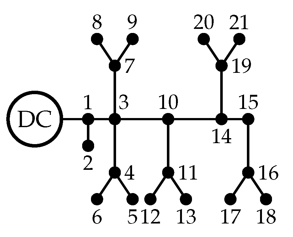
4.1. Bipolar DC 21-Bus System

The 21-node test system has a radial grid topology and was modified for bipolar DC network analysis in [28]. This test system has a substation located at bus 1, operating with a rated voltage of $\pm 1$ kV in the positive and negative poles, and its neutral pole is solidly grounded. The total power consumptions in the positive and negative poles are 554 kW and 445 kW, respectively, and the total power consumption for bipolar loads is 405 kW. Figure 3 depicts the single-line scheme of the system’s topology.

Table 1. Parametric data for the 21-bus system (all powers in kW).

Node j	Node k	${\mathit{R}}_{\mathit{jk}}$ ($\mathbf{\Omega }$)	${\mathit{P}}_{\mathit{dk}}^{\mathit{p}}$	${\mathit{P}}_{\mathit{dk}}^{\mathit{n}}$	${\mathit{P}}_{\mathit{dk}}^{\mathit{p}-\mathit{n}}$
1	2	0.053	70	100	0
1	3	0.054	0	0	0
3	4	0.054	36	40	120
4	5	0.063	4	0	0
4	6	0.051	36	0	0
3	7	0.037	0	0	0
7	8	0.079	32	50	0
7	9	0.072	80	0	100
3	10	0.053	0	10	0
10	11	0.038	45	30	0
11	12	0.079	68	70	0
11	13	0.078	10	0	75
10	14	0.083	0	0	0
14	15	0.065	22	30	0
15	16	0.064	23	10	0
16	17	0.074	43	0	60
16	18	0.081	34	60	0
14	19	0.078	9	15	0
19	20	0.084	21	10	50
19	21	0.082	21	20	0

shows the parametric data of this test system, along with the resistance values of the lines and the consumption load for each pole and between poles.

4.2. Bipolar DC 33-Bus System

The 33-node system also has a radial grid topology, and its version for bipolar DC grids was proposed in [29]. For this test system, the rated voltages in the substation (located at bus 1) are $\pm 12.66$ kV in the positive and negative poles, and its neutral pole is solidly grounded. The total power demand in the positive and negative poles is 2615 kW and 2185 kW, respectively, and the total power demand in bipolar loads is 2350 kW. Figure 4 illustrates the single-line scheme of the 33-bus system’s topology. The resistance values of the lines and consumption loads in each pole and between poles for the bipolar DC system are listed in

Table 2. Parametric data of the 33-bus system (all powers in kW).

Node j	Node k	${\mathit{R}}_{\mathit{jk}}$ ($\mathbf{\Omega }$)	${\mathit{P}}_{\mathit{dk}}^{\mathit{p}}$	${\mathit{P}}_{\mathit{dk}}^{\mathit{n}}$	${\mathit{P}}_{\mathit{dk}}^{\mathit{p}-\mathit{n}}$
1	2	0.0922	100	150	0
2	3	0.4930	90	75	0
3	4	0.3660	120	100	0
4	5	0.3811	60	90	0
5	6	0.8190	60	0	200
6	7	0.1872	100	50	150
7	8	1.7114	100	0	0
8	9	1.0300	60	70	100
9	10	1.0400	60	80	25
10	11	0.1966	45	0	0
11	12	0.3744	60	90	0
12	13	1.4680	60	60	100
13	14	0.5416	120	100	200
14	15	0.5910	60	30	50
15	16	0.7463	110	0	350
16	17	1.2890	60	90	0
17	18	0.7320	90	45	0
2	19	0.1640	90	150	0
19	20	1.5042	150	50	115
20	21	0.4095	0	90	0
21	22	0.7089	0	90	145
3	23	0.4512	90	110	35
23	24	0.8980	120	0	40
24	25	0.8960	150	100	100
6	26	0.2030	60	80	0
26	27	0.2842	60	0	225
27	28	1.0590	0	0	130
28	29	0.8042	120	75	65
29	30	0.5075	100	100	0
30	31	0.9744	50	150	125
31	32	0.3105	175	100	75
32	33	0.3410	95	60	120

.

4.3. Bipolar DC 85-Bus System

The 85-node test system has a radial grid topology, and its version for bipolar DC grids was described in [30]. For this test system, the rated voltages in the substation (located at bus 1) are $\pm 11$ kV in the positive and negative poles, and its neutral pole is solidly grounded. The total power demand in the positive and negative poles is $1745.48$ kW and $2682.19$ kW, respectively, and the total power demand for bipolar loads is $2258.58$ kW. Figure 5 illustrates the single-line scheme of the 85-node system’s topology. The resistance values of the lines and consumption loads in each pole and between poles for this DC system are listed in

Table 3. Parametric information of the 85-bus grid (all powers in kW).

Node j	Node k	${\mathit{R}}_{\mathit{jk}}$ ($\mathbf{\Omega }$)	${\mathit{P}}_{\mathit{dk}}^{\mathit{p}}$	${\mathit{P}}_{\mathit{dk}}^{\mathit{p}}$	${\mathit{P}}_{\mathit{dk}}^{\mathit{p}-\mathit{n}}$	Node j	Node k	${\mathit{R}}_{\mathit{jk}}$ ($\mathbf{\Omega }$)	${\mathit{P}}_{\mathit{dk}}^{\mathit{p}}$	${\mathit{P}}_{\mathit{dk}}^{\mathit{p}}$	${\mathit{P}}_{\mathit{dk}}^{\mathit{p}-\mathit{n}}$
1	2	0.108	0	0	10.075	34	44	1.002	17.64	17.995	0
2	3	0.163	50	0	40.35	44	45	0.911	50	17.64	17.995
3	4	0.217	28	28.565	0	45	46	0.911	25	17.64	17.995
4	5	0.108	100	50	0	46	47	0.546	7	7.14	10
5	6	0.435	17.64	17.995	25.18	35	48	0.637	0	10	0
6	7	0.272	0	8.625	0	48	49	0.182	0	0	25
7	8	1.197	17.64	17.995	30.29	49	50	0.364	18.14	0	18.505
8	9	0.108	17.8	350	40.46	50	51	0.455	28	28.565	0
9	10	0.598	0	100	0	48	52	1.366	30	0	15
10	11	0.544	28	28.565	0	52	53	0.455	17.64	35	17.995
11	12	0.544	0	40	45	53	54	0.546	28	30	28.565
12	13	0.598	45	40	22.5	52	55	0.546	38	0	48.565
13	14	0.272	17.64	17.995	35.13	49	56	0.546	7	40	32.14
14	15	0.326	17.64	17.995	20.175	9	57	0.273	48	35.065	10
2	16	0.728	17.64	67.5	33.49	57	58	0.819	0	50	0
3	17	0.455	56.1	57.15	50.25	58	59	0.182	18	28.565	25
5	18	0.820	28	28.565	200	58	60	0.546	28	43.565	0
18	19	0.637	28	28.565	10	60	61	0.728	18	28.565	30
19	20	0.455	17.64	17.995	150	61	62	1.002	12.5	29.065	0
20	21	0.819	17.64	70	152.5	60	63	0.182	7	7.14	5
21	22	1.548	17.64	17.995	30	63	64	0.728	0	0	50
19	23	0.182	28	75	28.565	64	65	0.182	12.5	25	37.5
7	24	0.910	0	17.64	17.995	65	66	0.182	40	48.565	33
8	25	0.455	17.64	17.995	50	64	67	0.455	0	0	0
25	26	0.364	0	28	28.565	67	68	0.910	0	0	0
26	27	0.546	110	75	175	68	69	1.092	13	18.565	25
27	28	0.273	28	125	28.565	69	70	0.455	0	20	0
28	29	0.546	0	50	75	70	71	0.546	17.64	38.275	17.995
29	30	0.546	17.64	0	17.995	67	72	0.182	28	13.565	0
30	31	0.273	17.64	17.995	0	68	73	1.184	30	0	0
31	32	0.182	0	175	0	73	74	0.273	28	50	28.565
32	33	0.182	7	7.14	12.5	73	75	1.002	17.64	6.23	17.995
33	34	0.819	0	0	0	70	76	0.546	38	48.565	0
34	35	0.637	0	0	50	65	77	0.091	7	17.14	25
35	36	0.182	17.64	0	17.995	10	78	0.637	28	6	28.565
26	37	0.364	28	30	28.565	67	79	0.546	17.64	42.995	0
27	38	1.002	28	28.565	25	12	80	0.728	28	28.565	30
29	39	0.546	0	28	28.565	80	81	0.364	45	0	75
32	40	0.455	17.64	0	17.995	81	82	0.091	28	53.75	0
40	41	1.002	10	0	0	81	83	1.092	12.64	32.995	62.5
41	42	0.273	17.64	25	17.995	83	84	1.002	62	72.2	0
41	43	0.455	17.64	17.995	0	13	85	0.819	10	10	10

.

5. Computational Results

Our recursive MIQ model was implemented in Matlab, using a Dell Inspiron 15 7000 Series computer (Intel Quad-Core [email protected] GHz) with 16 GB RAM and 64-bit Windows 10 Home Single Language. The model was run in a disciplined convex programming tool known as CVX for Matlab [31], and the Gurobi solver was employed [32].

The effectiveness of the proposed recursive MIQ model was evaluated and compared to the non-convex MINLP model in GAMS using the CBC, BONMIN, and GUROBI solvers [33]. Additionally, two simulation cases were considered:

C1:

The proposed recursive MIQ model and the non-convex MINLP model were assessed while only considering the grounding of the three neutral wires.

C2:

The impact on the total power losses caused by varying the number of neutral wires grounded from 0 to 5 was analyzed.

5.1. Analysis of Case 1 (C1)

This case was evaluated regarding the performance of the proposed recursive MIQ model, implemented in CVX while using the Gurobi solver. The model was also compared with its non-convex MINLP model solved using GAMS with three different available solvers. The numerical results of the objective function $p_{\mathrm{loss}}$ for the three tested bipolar DC grids are listed in

Table 4. Optimal neutral grounding found by the proposed recursive MIQ model and the GAMS solvers.

	21-Bus Bipolar DC Grid		33-Bus Bipolar DC Grid		85-Bus Bipolar DC Grid
Method	Location (Bus)	${\mathit{p}}_{\mathrm{loss}}$(kW)	Location (Bus)	${\mathit{p}}_{\mathrm{loss}}$(kW)	Location (Bus)	${\mathit{p}}_{\mathrm{loss}}$(kW)
Ben. case		95.4237		344.4797		489.5759
CBC	$\{6,9,17\}$	91.5346	$\{16,21,25\}$	336.0032	$\{20,25,72\}$	455.5865
BONMIN	$\{9,18,20\}$	92.1718	$\{18,24,31\}$	335.9671	$\{56,57,74\}$	455.5984
GUROBI	$\{9,17,18\}$	91.7213	$\{16,17,18\}$	336.7072	$\{32,33,69\}$	459.3622
MIQ	$\{6,9,17\}$	91.5346	$\{6,16,24\}$	334.9963	$\{9,32,64\}$	453.3122

.

Based on Table 4, it can be stated that

• The proposed recursive MIQ model reached the best solution in the analyzed networks, with objective function values of 91.5346 kW, 335.0946 kW, and 453.3122 kW for the bipolar DC 21-, 33-, and 85-node systems, respectively. These results were also obtained by the non-convex MINLP model. In addition, the results show power loss reductions of 4.07%, 2.75%, and 7.40% (compared to the benchmark cases) for the bipolar DC 21-, 33-, and 85-node test feeders.
• For the bipolar DC 21-bus system, it can be observed that the CBC solver found the same result as the recursive MIQ model. In comparison, the other solvers (BONMIN and GUROBI) achieved the worst solutions; they became stuck in local optima. These results reduced the power losses by 3.40% and 3.88%.
• For the bipolar DC 33-bus system, it can be noted that no GAMS solver could find the same solution as the proposed model; they all reached different local optima, reducing the power losses by 2.46%, 2.47%, and 2.25% for the CBC, BONMIN, and GUROBI solvers, respectively.
• For the bipolar DC 85-bus system, no GAMS solver could reach the same solution as the proposed model, and the solutions differ. This indicates that the GAMS solvers found local optima, reducing the grid power losses by 6.94%, 6.94%, and 6.17%, that is, the CBC, BONMIN, and GUROBI solvers, respectively.
• No GAMS solver outperformed the others, since the CBC solver found a better solution in the bipolar DC 21- and 85-node systems, while the BONMIN solver reached a better solution for the 33-bus system.

A comparison of the voltage profiles between the benchmark cases and the recursive MIQ model for the bipolar DC systems is depicted in Figure 6. Figure 6a–c show the voltage profiles of the positive, neutral, and negative poles for the 21-bus bipolar system, respectively. Figure 6d–f present the voltage profiles of the positive, neutral, and negative poles for the 33-bus bipolar system. Finally, Figure 6g–i show the voltage profiles of the positive, neutral, and negative poles for the 21-bus bipolar system.

From the voltage profiles presented in Figure 6, it is possible to state that the grounding of the neutral wire in three nodes can improve the voltage balance in bipolar DC grids. Note that, in Figure 6b,e,h, the neutral pole voltages are improved, keeping these voltages closer to zero and reducing their standard deviation by 16.99%, 89.59%, and 89.33%, respectively.

5.2. Analysis of Case 2 (C2)

This case involves the impact of increasing the neutral grounding on power losses. Figure 7 depicts the reduction in power losses considering 1 to 5 grounded nodes and complete neutral grounding.

Figure 7 shows that, after the third grounded node, the impact of reducing power losses in bipolar networks is not significant. This can be supported by looking at the power losses reductions regarding three grounded nodes and complete grounding, whose differences are imperceptible for the bipolar DC systems. In these intervals, the reductions in power losses are 0.29%, 0.17%, and 0.22% for the bipolar DC 21-, 33-, and 85-bus systems, respectively.

Table 5. Selected grounding neutral nodes for bipolar DC networks.

Number of Nodes for Grounding	Grounded Nodes
	21-Test System	33-Test System	85-Test System
1	$\left[\begin{array}{c}9\end{array}\right]$	$\left[\begin{array}{c}16\end{array}\right]$	$\left[\begin{array}{c}9\end{array}\right]$
2	$\left[\begin{array}{c}9,17\end{array}\right]$	$\left[\begin{array}{c}6,16\end{array}\right]$	$\left[\begin{array}{c}9,32\end{array}\right]$
3	$\left[\begin{array}{c}6,9,17\end{array}\right]$	$\left[\begin{array}{c}6,16,24\end{array}\right]$	$\left[\begin{array}{c}9,32,64\end{array}\right]$
4	$\left[\begin{array}{c}6,9,17,18\end{array}\right]$	$\left[\begin{array}{c}8,16,24,29\end{array}\right]$	$\left[\begin{array}{c}9,12,29,64\end{array}\right]$
5	$\left[\begin{array}{c}6,9,13,17,18\end{array}\right]$	$\left[\begin{array}{c}8,16,24,27,33\end{array}\right]$	$\left[\begin{array}{c}9,12,29,32,64\end{array}\right]$

presents the nodes selected for grounding by our recursive MIQ model.

From the results listed in Table 5, it can be stated that, in the three DC bipolar networks, the same node is always selected, which implies that it has greater participation in reducing power losses.

6. Conclusions and Future Works

This study addressed the issue of optimal grounding for the neutral wire in bipolar DC networks with asymmetric loading. This, by reformulating the non-convex MINLP model as a recursive MIQ model via the linearization of the hyperbolic relation between voltage and power at each node. This linearization relaxed the aforementioned hyperbolic relation in constant power terminals. A recursive algorithm was utilized to eliminate the possible errors generated by linearization. The recursive MIQ model was evaluated in three bipolar DC systems and compared to three solvers of the GAMS software. The results showed that the MIQ model reached the global optimum of the problem, reducing the power losses by 4.08%, 2.75%, and 7.40% for bipolar DC systems of 21, 33, and 85 buses when considering three grounded nodes. For the DC 21-bus bipolar system only, one of the GAMS software solvers also found the same solution as our MIQ model. In the other cases, these solvers failed and reached local optima. The recursive MIQ model generally showed a superior performance to that of the GAMS solvers.

The impact of grounding the neutral wire in bipolar DC networks was analyzed by varying the number of available nodes to be grounded (0 to 5), demonstrating that the reduction in power losses is imperceptible after three grounded nodes, as these reductions showed values of 0.29%, 0.17%, and 0.22% for the bipolar DC 21-, 33-, and 85-node systems, respectively.

Future works could be extended the proposed model to bipolar DC networks with a high presence of distributed energy resources.

References

1. Lakshmi, S.; Ganguly, S. Transition of Power Distribution System Planning from Passive to Active Networks: A State-of-the-Art Review and a New Proposal. In Sustainable Energy Technology and Policies; Springer: Singapore, 2017; pp. 87–117. [Google Scholar] [CrossRef]
2. Liu, G.; Huang, R.; Pu, T.; Yang, Z. Design of energy management system for Active Distribution Network. In Proceedings of the 2014 China International Conference on Electricity Distribution (CICED), Shenzhen, China, 23–26 September 2014. [Google Scholar] [CrossRef]
3. Li, Z.; Su, S.; Zhao, Y.; Jin, X.; Chen, H.; Li, Y.; Zhang, R. Energy management strategy of active distribution network with integrated distributed wind power and smart buildings. IET Renew. Power Gener. 2020, 14, 2255–2267. [Google Scholar] [CrossRef]
4. Zhou, D.; Chen, S.; Wang, H.; Guan, M.; Zhou, L.; Wu, J.; Hu, Y. Autonomous Cooperative Control for Hybrid AC/DC Microgrids Considering Multi-Energy Complementarity. Front. Energy Res. 2021, 9, 692026. [Google Scholar] [CrossRef]
5. Siraj, K.; Khan, H.A. DC distribution for residential power networks—A framework to analyze the impact of voltage levels on energy efficiency. Energy Rep. 2020, 6, 944–951. [Google Scholar] [CrossRef]
6. Jing, G.; Zhang, A.; Zhang, H. Review on DC Distribution Network Protection Technology with Distributed Power Supply. In Proceedings of the 2018 Chinese Automation Congress (CAC), Xi’an, China, 30 November–2 December 2018. [Google Scholar] [CrossRef]
7. Liu, Z.; Li, M. Research on Energy Efficiency of DC Distribution System. AASRI Procedia 2014, 7, 68–74. [Google Scholar] [CrossRef]
8. Garces, A. Uniqueness of the power flow solutions in low voltage direct current grids. Electr. Power Syst. Res. 2017, 151, 149–153. [Google Scholar] [CrossRef]
9. Garces, A. On the Convergence of Newton’s Method in Power Flow Studies for DC Microgrids. IEEE Trans. Power Syst. 2018, 33, 5770–5777. [Google Scholar] [CrossRef]
10. Justo, J.J.; Mwasilu, F.; Lee, J.; Jung, J.W. AC-microgrids versus DC-microgrids with distributed energy resources: A review. Renew. Sustain. Energy Rev. 2013, 24, 387–405. [Google Scholar] [CrossRef]
11. Razmi, D.; Babayomi, O.; Davari, A.; Rahimi, T.; Miao, Y.; Zhang, Z. Review of Model Predictive Control of Distributed Energy Resources in Microgrids. Symmetry 2022, 14, 1735. [Google Scholar] [CrossRef]
12. Zhu, H.; Zhu, M.; Zhang, J.; Cai, X.; Dai, N. Topology and operation mechanism of monopolar-to-bipolar DC-DC converter interface for DC grid. In Proceedings of the 2016 IEEE 8th International Power Electronics and Motion Control Conference (IPEMC-ECCE Asia), Hefei, China, 22–26 May 2016. [Google Scholar] [CrossRef]
13. Najafi, P.; Viki, A.H.; Shahparasti, M. An integrated interlinking converter with DC-link voltage balancing capability for bipolar hybrid microgrid. Electr. Eng. 2019, 101, 895–909. [Google Scholar] [CrossRef]
14. Montoya, O.D.; Grisales-Noreña, L.F.; Gil-González, W. Optimal Pole-Swapping in Bipolar DC Networks with Multiple CPLs Using an MIQP Model. IEEE Trans. Circuits Syst. II Express Briefs 2023. [Google Scholar] [CrossRef]
15. Liao, J.; Zhou, N.; Wang, Q.; Chi, Y. Load-Switching Strategy for Voltage Balancing of Bipolar DC Distribution Networks Based on Optimal Automatic Commutation Algorithm. IEEE Trans. Smart Grid 2021, 12, 2966–2979. [Google Scholar] [CrossRef]
16. Chew, B.S.H.; Xu, Y.; Wu, Q. Voltage Balancing for Bipolar DC Distribution Grids: A Power Flow Based Binary Integer Multi-Objective Optimization Approach. IEEE Trans. Power Syst. 2019, 34, 28–39. [Google Scholar] [CrossRef]
17. Montoya, O.D.; Medina-Quesada, Á.; Hernández, J.C. Optimal Pole-Swapping in Bipolar DC Networks Using Discrete Metaheuristic Optimizers. Electronics 2022, 11, 2034. [Google Scholar] [CrossRef]
18. Lee, J.O.; Kim, Y.S.; Jeon, J.H. Generic power flow algorithm for bipolar DC microgrids based on Newton–Raphson method. Int. J. Electr. Power Energy Syst. 2022, 142, 108357. [Google Scholar] [CrossRef]
19. Montoya, O.D.; Gil-González, W.; Hernández, J.C. Optimal Power Flow Solution for Bipolar DC Networks Using a Recursive Quadratic Approximation. Energies 2023, 16, 589. [Google Scholar] [CrossRef]
20. Garces, A.; Montoya, O.D.; Gil-Gonzalez, W. Power Flow in Bipolar DC Distribution Networks Considering Current Limits. IEEE Trans. Power Syst. 2022, 37, 4098–4101. [Google Scholar] [CrossRef]
21. Montoya, O.D.; Gil-González, W.; Garcés, A. A successive approximations method for power flow analysis in bipolar DC networks with asymmetric constant power terminals. Electr. Power Syst. Res. 2022, 211, 108264. [Google Scholar] [CrossRef]
22. Mackay, L.; Dimou, A.; Guarnotta, R.; Morales-Espania, G.; Ramirez-Elizondo, L.; Bauer, P. Optimal power flow in bipolar DC distribution grids with asymmetric loading. In Proceedings of the 2016 IEEE International Energy Conference (ENERGYCON), Leuven, Belgium, 4–8 April 2016. [Google Scholar] [CrossRef]
23. Mackay, L.; Guarnotta, R.; Dimou, A.; Morales-Espana, G.; Ramirez-Elizondo, L.; Bauer, P. Optimal Power Flow for Unbalanced Bipolar DC Distribution Grids. IEEE Access 2018, 6, 5199–5207. [Google Scholar] [CrossRef]
24. Montoya, O.D.; Grisales-Noreña, L.F.; Hernández, J.C. A Recursive Conic Approximation for Solving the Optimal Power Flow Problem in Bipolar Direct Current Grids. Energies 2023, 16, 1729. [Google Scholar] [CrossRef]
25. Lee, J.O.; Kim, Y.S.; Jeon, J.H. Optimal power flow for bipolar DC microgrids. Int. J. Electr. Power Energy Syst. 2022, 142, 108375. [Google Scholar] [CrossRef]
26. Barbu, V.; Precupanu, T. Convexity and Optimization in Banach Spaces; Springer: Dordrecht, The Netherlands, 2012. [Google Scholar] [CrossRef]
27. Berkovitz, L.D. Convexity and Optimization in Rn, 1st ed.; Wiley-Interscience: Hoboken, NJ, USA, 2001. [Google Scholar]
28. Montoya, O.D.; Molina-Cabrera, A.; Gil-González, W. A mixed-integer convex approximation for optimal load redistribution in bipolar DC networks with multiple constant power terminals. Results Eng. 2022, 16, 100689. [Google Scholar] [CrossRef]
29. Montoya, O.D.; Gil-González, W.; Hernández, J.C. Optimal Scheduling of Photovoltaic Generators in Asymmetric Bipolar DC Grids Using a Robust Recursive Quadratic Convex Approximation. Machines 2023, 11, 177. [Google Scholar] [CrossRef]
30. Sepúlveda-García, S.; Montoya, O.D.; Garcés, A. Power Flow Solution in Bipolar DC Networks Considering a Neutral Wire and Unbalanced Loads: A Hyperbolic Approximation. Algorithms 2022, 15, 341. [Google Scholar] [CrossRef]
31. Grant, M.; Boyd, S. CVX: Matlab Software for Disciplined Convex Programming, Version 2.1. 2014. Available online: http://cvxr.com/cvx (accessed on 28 March 2023).
32. Gurobi Optimization, LLC. Gurobi Optimizer Reference Manual; Gurobi Optimization, LLC: Beaverton, OR, USA, 2023. [Google Scholar]
33. Soroudi, A. Power System Optimization Modeling in GAMS; Springer International Publishing: Cham, Switzerland, 2017. [Google Scholar] [CrossRef]
Figure 1. Possible grid topologies for DC distribution networks: (a) monopolar and (b) bipolar.
Energies 16 03755 g001
Figure 2. Flowchart for the recursive MIQ model (26)–(41).
Energies 16 03755 g002
Figure 3. Single-line scheme of the bipolar 21-bus system.
Energies 16 03755 g003
Figure 4. Single-line scheme of the bipolar 33-bus system.
Energies 16 03755 g004
Figure 5. Single-line scheme of the bipolar 85-bus system.
Energies 16 03755 g005
Figure 6. Comparison of the voltage profiles, the benchmark cases vs. optimal neutral grounding: (a,d,g): voltage profiles of the positive pole; (b,e,h): voltage profiles of the neutral pole; and (c,f,i): voltage profiles of the negative pole.
Energies 16 03755 g006
Figure 7. Percentage of power losses regarding the benchmark case by number of grounded neutral nodes.
Energies 16 03755 g007