Abstract
Studies have reported the incorporation of microorganisms into cement to promote the formation of calcium carbonate in cracks of concrete, a process known as biomineralization. The paper aims to improve the process of the cascade system for biomineralization in cement by identifying the best hydrodynamic conditions in a reaction cell in order to increase the useful life of concrete structures and, therefore, bring energy and environmental benefits. Two central composite rotatable designs were used to establish the positioning of the air inlet and outlet in the lateral or upper region of the geometry of the reaction cell. The geometries of the reaction cell were constructed in SOLIDWORKS®, and computational fluid dynamics was performed using the Flow Simulation tool of the same software. The results were submitted to statistical analysis. The best combination of meshes for the simulation was global mesh 4 and local mesh 5. The statistical analysis applied to gas velocity and pressure revealed that air flow rate was the factor with the greatest sensitivity, with values up to 99.9%. The geometry with the air outlet and inlet in the lateral region was considered to be the best option.
1. Introduction
Concrete, the most widely used construction material in the world, consists of cement, fine and coarse aggregates, and water mixed in suitable proportions and is employed in all types of civil engineering projects, such as street surfaces, buildings, residences, and bridges. The wide availability of components, long durability, and favorable cost–benefit ratio are the main reasons for the universal use of concrete in civil construction [1,2,3].
However, the low tensile strength makes concrete susceptible to the formation of cracks, which places the durability of concrete structures at risk. Cracks and microcracks can lead to the deterioration of concrete structures, as aggressive liquids and gases can penetrate the matrix and diminish the mechanical performance of such structures. The use of self-healing concrete with a crack-healing mechanism triggered without human intervention would be a highly beneficial solution for this problem [4].
Different types of microbial agents have recently been incorporated into concrete to promote the healing of cracks through the precipitation of microbiologically induced calcium carbonate (CaCO3) [5,6]. The biochemical process in which microorganisms induce mineral precipitation is known as biomineralization [7]. This phenomenon usually takes place when the organic matter is transformed, for any protecting or nutrition function, by microorganisms (mainly bacteria and fungi) into inorganic compounds, mainly calcium carbonate. The biomineralization of carbonate using microorganisms brings some benefits to the concrete industry, such as increased concrete strength and compatibility of carbonate with concrete, since this compound is one of the constituents of cement, in addition to the advantage of being an environmentally correct option, which can reduce cement production. The mineral resulting from the microbiologically induced calcium carbonate precipitation may be in any of the three CaCO3 polymorphs, i.e., calcite, vaterite, or aragonite. Calcite is preferable for bacteria-based self-generating concrete due to its greater thermodynamic stability. The different pathways by which microorganisms are able to produce calcium carbonate are broadly classified as autotrophic or heterotrophic [8,9]. The heterotrophic group includes the oxidation of organic salts such as calcium lactate, which is the simplest and safest pathway (Equation (1)):
while the carbonation of calcium hydroxide to calcium carbonate is likely to occur both chemically and through the action of autotrophic microorganisms (Equation (2)):
The seasonality of temperatures favors the formation of cracks in concrete due to thermal retraction and expansion, resulting in greater thermal resistance of the concrete. Even though air is a poor conductor of heat, under unfavorable conditions hot regions can form in areas of factories, leading to unsuitable temperatures for workers and contributing to a reduction in structure energetic effectiveness. In cases related to bridges, temperature changes can cause structure thermal expansion, which generates the need for periodic maintenance. Promising investigations regarding self-healing concrete are being carried out with the aim of creating possibilities for eco-sustainable and energy-efficient ways to seal cracks in concrete [8].
The construction sector consumes 40% of the world’s energy and is responsible for about 30% of greenhouse gas emissions, generated mainly by the production of building materials (such as those made in the steel, cement, and glass industries) and their transport, as well as the construction, installation, and decoration of buildings and renovation, maintenance, and demolition activities, among others [10,11]. A study carried out by Zhu et al. [11] demonstrated that reduction in carbon emissions in the construction sector is linked mainly to the implementation of energy-saving technologies in the steel, cement, and construction industries, which have also improved industrial production and reduced product prices. Zhang et al. [12] analyzed the use of the latest data-driven algorithms to predict the health status of lithium-ion batteries (LIBs) and proposed a general prediction process, including the acquisition of datasets for LIBs’ charging and discharging process, data processing, features, and algorithm selection. LIBs can be a promising alternative to mitigate the effects of greenhouse gases and contribute to energy issues, as they have been used in various sectors due to their significant advantages. The high level of accuracy in estimating battery health greatly increases safety and process reliability. Another excellent alternative are the technologies developed on the subject of self-healing concrete, which can also help reduce greenhouse gases and energy consumption, mainly because they increase the useful life of concrete structures.
Oxygen availability is a significant variable that affects the biomineralization of CaCO3. Aerobic organisms use oxygen to grow, leading to the production of bioproducts under certain conditions. Considering the robustness of bacterial groups in the exponential growth phase and their significant role in the biomineralization of CaCO3, ensuring conditions capable of enhancing bacterial growth is of paramount importance [13].
The design of experiments has been widely used in different fields of science and industry to develop and optimize products and processes. It resorts to a set of statistical tools aimed at systematically classifying and quantifying cause-and-effect relationships between variables and outcomes in the process or phenomenon to be studied, which can result (if this is the objective) in finding the configurations and conditions under which it is optimized. The main objective of experimental design is to obtain the maximum quantity of information to limit the number of necessary observations and therefore reduce the total number of experiments needed [14,15].
Classic methods of experimental designing include complete factorial design, Plackett–Burman design, central composite design, central composite rotatable design (CCRD), and Box–Behnken design [16]. CCRD is a type of experimental design that enables the investigation of the effects of multiple variables simultaneously. This method has the additional benefit of requiring fewer experiments, and the results of the experiments enable the determination of three-dimensional response surfaces and empirical mathematical models for each response variable [17].
Even though the experimental elucidation of the mechanisms behind a phenomenon is preferable due to the predictability of possible unforeseen events, the consumption of resources and the limited number of experiments that can be conducted in practice may render the obtainment of results concordant with reality unfeasible [18]. Computational fluid dynamics (CFD) is a computer-based method to characterize, interpret, and quantify fluid transport phenomena through a numeric solution of the Navier–Stokes equations capable of replicating realistic scenarios with a three-dimensional (3D) domain under unstable conditions [19]. The Navier–Stokes formulations are equations of mass conservation, momentum conservation, and energy conservation (Equations (3)–(5), respectively) [20]:
where is the time, is the vector velocity, is the stress tensor, is the density, is the static pressure, is the gravitational acceleration vector, is the thermal conductivity, is the standard enthalpy, and is the temperature [20].
One of the most important requirements for CFD is the generation of the mesh size, the knowledge of whose influence is essential to produce precise results. The analysis of different variables and the assessment of numerical results by comparison with classic solutions enable obtaining an adequate mesh for a specific problem. The mesh generation process is considered a pre-processing step, as it is necessary prior to the solution of the Navier–Stokes equations. The mesh is a data structure that contains all location and topology information of the discretized domain, playing a critical role in the computational efficiency and precision of the solution. Due to the complexity and diversity of the geometries, meshing has always been a complex process since the emergence of CFD and has been widely studied in different fields of CFD, structure analysis, and other fields of engineering [21,22].
CFD can be used since the conceptual phase of a project to determine its viability and the best solution for the study to be carried out and allow to represent various scenarios. Therefore, this tool was used in this study, with the aid of experimental designs, to identify the best hydrodynamic conditions in reactive cell for biomineralization, aiming to improve the process of the cascade system for biomineralization in cement, in order to increase the useful life of concrete structures and to ensure great energy and environmental benefits.
2. Materials and Methods
The present study was conducted to assist, guide, and maximize the results of the cascade system for biomineralization in cement developed by Brasileiro et al. [23] and displayed in Figure 1.
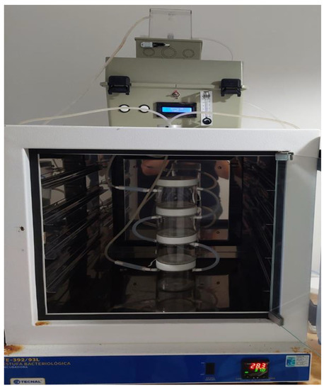
Figure 1.
Cascade system used to perform biomineralization in cement.
The construction of the system began with the filtering of data from the solubility curve in the typical temperature range of the biomineralization process (5–35 °C). The aim of the curve is to predict the maximum saturation threshold at each temperature to work under conditions from the non-crystallization of water (above the freezing point) to the optimal temperature (35 °C) for bacteria of the genus Bacillus. The volumetric air flow rate of the system ranged from 0.5 to 4.0 L·min−1 [23].
2.1. Conceptual Model of Reaction Cells
The conceptual models of the reaction cells were conceived in two different forms, differing in terms of position of the air inlet and outlet. Both the inlet and outlet were in the lateral region in the former model (Figure 2a) and in the upper region in the latter (Figure 2b). Both were composed of four basis parameters:
- Air flow rate (Q);
- Diameter of reaction cell ();
- Distance of air inlet ();
- Distance of air outlet ().

Figure 2.
Conceptual model of reaction cell with air inlet and outlet (a) in the lateral region and (b) in the upper region.
2.2. Construction of Geometries of Reaction Cells
The geometries of the reaction cells were constructed using the SOLIDWORKS® 2020 software (Dassault Systèmes, Vélizy-Villacoublay, France). Each was developed in accordance with the dimensions specified in the factorial design described in the next subsection and respecting the position of the air inlets and outlets displayed in Figure 2.
The material defined for the geometries was glass, the properties of which are defined according to the library of materials predetermined in the software.
The construction of the geometries was complemented with some standard dimensions used in all geometries produced, as shown in Table 1.

Table 1.
Standard construction dimensions used for reaction cells.
2.3. Factorial Designs for Investigation of Oxygen Distribution in the Reaction Cells
The experiments were conducted following two factorial CCRDs, as this type of experimental design has greater division of levels and greater analysis properties of the estimated effects than others. Four variables were studied for each factorial design. Both CCRDs had +2.00 and −2.00 cubic level, the steps were the same, and the total number of experiments was 28 [24]. However, the use of CFD applied to the CCRD data generates the absence of unforeseen events, resulting in 25 runs for each factorial design, with the discarding of runs 26 to 28, which were repetitions of run 25.
The two factorial designs were divided according to the position of the air inlets and outlets (lateral and upper regions of the reaction cell geometry); therefore, they were denominated: (1) lateral inlet and outlet factorial design and (2) upper inlet and outlet factorial design.
2.3.1. Lateral Inlet and Outlet Factorial Design
The variables of interest in the lateral inlet and outlet factorial design were air flow rate (L/min), reaction cell diameter (cm), distance of air inlet (cm), and distance of air outlet (cm). Table 2 lists the coded values of the levels, the diameter of the reaction cell, and the distance of both the air inlet and air outlet, while Table 3 summarizes the matrix of runs, whose results served as a basis to help the construction of such a geometry.
Table 2.
Matrix of levels used in the factorial design for the lateral inlet and outlet configuration.
Table 3.
Matrix of runs performed according to the lateral inlet and outlet factorial design.
2.3.2. Upper Inlet and Outlet Factorial Design
The variables of interest in the upper inlet and outlet factorial design were the same as for the one presented in the previous subsection, with Table 4 and Table 5 summarizing the corresponding coded values of levels and run matrix. The values gathered in Table 5 served as the basis for the construction of such a geometry.
Table 4.
Matrix of levels used in the factorial design for the upper inlet and outlet configuration.
Table 5.
Matrix of runs performed according to the upper inlet and outlet factorial design.
2.4. Computational Flow Dynamics
Numerical models were constructed in SOLIDWORKS®, and the simulation study was performed using the Flow Simulation tool of the software. SOLIDWORKS® Flow Simulation is a new class of CFD analysis software used for the study of fluid transport phenomena [25].
The Q values listed in Table 3 and Table 5, together with the specific parameters listed in Table 6, were adjusted in SOLIDWORKS®, and computational simulations were performed using the selected geometries of the reaction cells.
Table 6.
Operating parameters used in simulations.
2.5. Mesh Convergence Study
The mesh convergence study consists of determining if the mesh is sufficiently refined to identify flow characteristics and to obtain more reliable results. For this purpose, a comparative analysis of two or more meshes with different degrees of refinement is suggested [26]. In this study, all geometries were used, as addressed in Section 2.2, using the working parameters listed in Table 6.
The global mesh defined for all geometries of the reaction cells was level 4 (ranging from level 1 to 7 according to the standard configuration of the software). To perform the mesh convergence study, it was necessary to make local refinements in the regions of greater flow of the geometry (inlets and outlets). For these local refinements (ranging from level 0 to 9 according to the standard configuration of the software), levels 0 to 6 were analyzed. To make this study possible, a line was traced in the outlet region of each cell vertical to the flow of the fluid in the central region of the tube and 1 cm from the end of the tube, as shown in Figure 3. The aim was to capture the entire velocity profile along the line to obtain data from all refinements and to perform graphic analyses to enable defining the best mesh for the development of simulations.
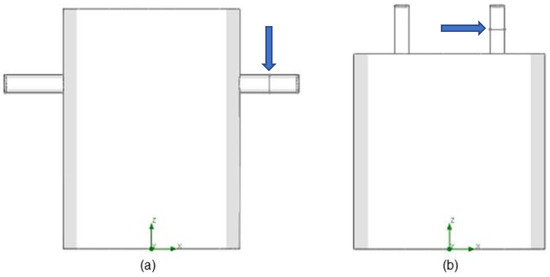
Figure 3.
(a) Model of geometry of lateral inlet and outlet with line traced to 1 cm from the end of the air outlet tube; (b) Model of geometry of upper inlet and outlet with line traced to 1 cm from the end of the air outlet tube.
2.6. Velocity and Pressure Studies
After the definition of the best meshes to be used in the simulations, air velocity and pressure set in the reaction cells were investigated. Two different analyses were performed for these variables, i.e., a global analysis of the two factors and a personalized one in a region of interest in which the position of a biocement layer is projected for future works. This region was located at a distance of 7 cm from the upper region of the object, and a line was established according to the diameter of each geometry, as shown in Figure 4. Data from some points on this line were captured through interpolations with the aim of visualizing velocity and pressure behavior in this particular region, the data of which can serve for subsequent statistical analyses.
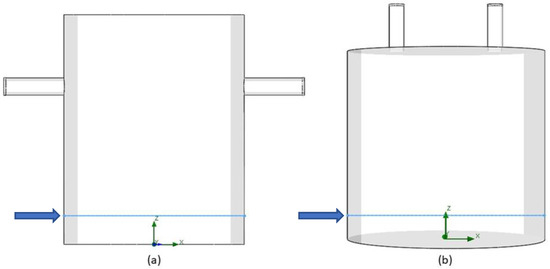
Figure 4.
(a) Model of geometry with lateral inlet and outlet with line drawn at 7 cm from the upper region of reaction cell; (b) Model of geometry with upper inlet and outlet with line drawn at 7 cm from the upper region of reaction cell.
2.7. Statistical Analysis
The velocity and pressure results in a specific region obtained in Section 2.6 were used for the statistical analyses with the aid of the Statistica 10.0 program (StatSoft, Tulsa, OK, USA) for the modeling of data.
3. Results
The mesh convergence study, investigations using CFD simulations for velocity and pressure, and statistical analysis were performed to determine the best operating conditions.
3.1. Mesh Convergence Study
The mesh convergence study was evaluated using different graphs made from the results of computational simulations. A tendency toward convergence was found in all the cases studied. The main variable in this study was velocity, through which the time of the central processing unit (CPU) employed in each refinement was also used for all runs. It is evident in Figure 5 and Figure 6, which illustrate the results of the analysis of velocity versus length for the different refinements, the formation of parabolas in all the cases studied, which may be associated with the fact that the flow was fully developed. Therefore, the velocity profile was parabolic for laminar flow, which is the case of this study. Dispersion occurred in the initial refinements, but the behavior of the curves tended to stabilize and converge with further refinement of the region of interest in such a way that one curve overlapped the others.
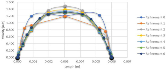
Figure 5.
Velocity versus length for different mesh refinements for geometry with lateral air inlet and outlet.
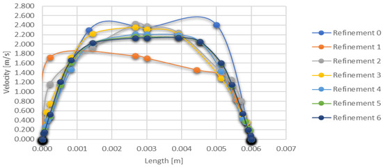
Figure 6.
Velocity versus length for different mesh refinements for the geometry with upper air inlet and outlet.
Figure 7 and Figure 8 show the behavior of the maximum velocity of each refinement versus the total number of mesh cells. Linearity was found in all cases, as the curve tended to converge independently of the increase in the total number of cells.
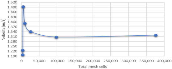
Figure 7.
Maximum velocity of each refinement versus total number of mesh cells for the geometry with lateral air inlet and outlet.
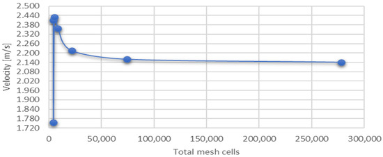
Figure 8.
Maximum velocity of each refinement versus total number of mesh cells for the geometry with upper air inlet and outlet.
From Figure 9 and Figure 10, which show the results of the analysis of CPU time versus the total number of mesh cells, it is evident the disparity found among the parameters in all runs, especially in the last two points of the graph, which refer to level 5 and level 6 refinement. The total number of mesh cells grew by three or four times when the refinement level was increased from 5 to 6, and the computational effort was correspondingly higher.
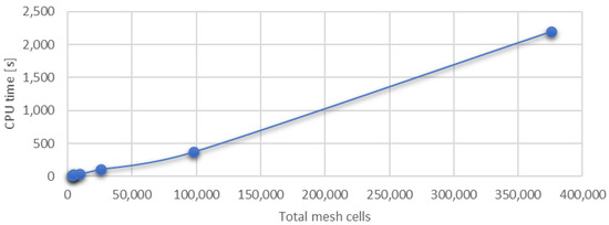
Figure 9.
Time of central processing unit (CPU) versus total number of mesh cells for the geometry with lateral air inlet and outlet.
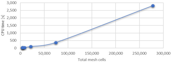
Figure 10.
Time of central processing unit (CPU) versus total number of mesh cells for the geometry with upper air inlet and outlet.
Table 7 and Table 8 list the representations of the best combinations of global and local meshes for each run, the numbers of mesh cells, and operating times generated by these mesh combinations for the geometries with lateral and upper air inlet and outlet, respectively. In both models, the local mesh of refinement on level 5 was considered the most adequate for simulations based on the entire graphic analysis, and the global mesh on level 4 was selected with the aim of greater precision in the results.
Table 7.
Representation of best combinations of global and local meshes for each run, number of mesh cells, and time of central processing unit (CPU) generated by these mesh combinations for the geometry with lateral air inlet and outlet.
Table 8.
Representation of best combinations of global and local meshes for each run, number of mesh cells, and time of central processing unit (CPU) generated by these mesh combinations for the geometry with upper air inlet and outlet.
Figure 11 and Figure 12 depict the best topologies of the discretized domains of the meshes after the convergence study for the two models of geometric configuration.
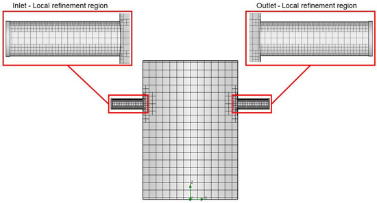
Figure 11.
Representation of mesh created after definition of global and local meshes for the geometry with lateral air inlet and outlet.
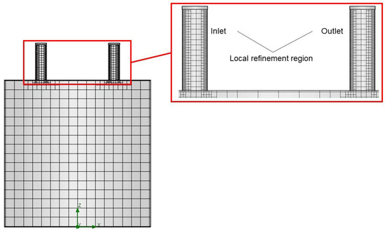
Figure 12.
Representation of mesh created after definition of global and local meshes for the geometry with upper air inlet and outlet.
3.2. Results of CFD Simulation for Velocity and Pressure
The results of the CFD simulations for velocity and pressure revealed some tendencies regardless of the type of selected geometry.
As shown in Figure 13 and Figure 14 as well as Figures S1–S48 of the Supplementary Material, air flow rate (L/min) exerted the greatest impact on the air velocity in the reaction cells in all the runs. In particular, the higher the values of Q used in the simulations, the higher those of air velocity.
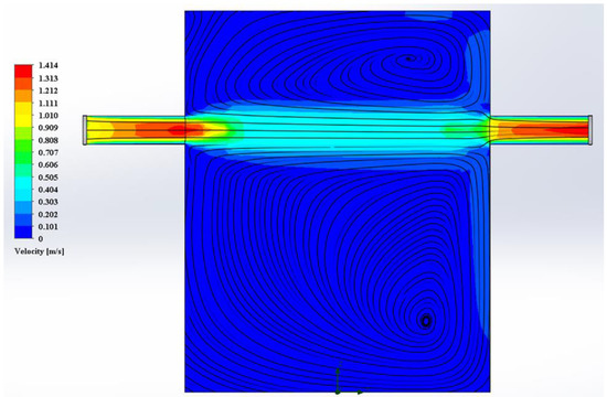
Figure 13.
Air velocity in reaction cell and current lines, in run 1, for the geometry with lateral air inlet and outlet. Q = 1.5 L/min; = 6.0 cm; = 2.5 cm; = 2.5 cm.
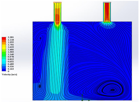
Figure 14.
Air velocity in reaction cell and current lines, in run 1, for the geometry with upper air inlet and outlet. Q = 2.5 L/min; = 8.0 cm; = 2.0 cm; = 2.0 cm.
As shown in Figure 15 and Figure 16 as well as Figures S49–S96 of the Supplementary Material, which correspond to the internal pressure of the reaction cell, moderate pressure variation was found for all geometries, with values around the previously established working parameter (101,325 Pa—standard atmospheric pressure at average sea level).
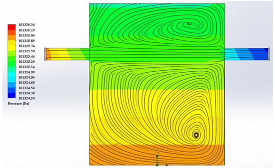
Figure 15.
Internal pressure in the reaction cell and current lines, in run 1, for the geometry with lateral air inlet and outlet. Q = 1.5 L/min; = 6.0 cm; = 2.5 cm; = 2.5 cm.
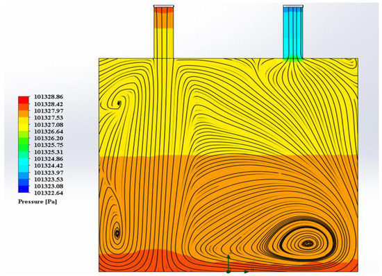
Figure 16.
Internal pressure in the reaction cell and current lines, in run 1, for the geometry with upper air inlet and outlet. Q = 2.5 L/min; = 8.0 cm; = 2.0 cm; = 2.0 cm.
The current lines presented in all models for velocity and pressure for both geometries reveal the trajectory of air particles in the form of lines. One can see that the reaction cell is completely filled with air, demonstrating excellent air availability in the cell.
Comparing the above figures showing air velocity and internal pressure in the reaction cells, one can consider the effects of Bernoulli’s principle on these resolutions, even with the discrete pressure values.
3.3. Statistical Analysis of Velocity and Pressure Results Obtained in a Specific Region
The representation of a given phenomenon through a model is often time-consuming, reflecting the concern with finding a more adequate path in the search of an optimization. The table of effects, analysis of variance (ANOVA), analysis of residuals, contour graphs, and surface graphs are essential tools to drive researchers in the direction they should follow.
Therefore, the results of internal pressure and air velocity, which were selected as responses in the present study, were analyzed via CFD in a specific region for factorial design with lateral and upper inlets and outlets to propose the best conditions aiming to optimize the process.
3.3.1. Geometry with Lateral Air Inlet and Outlet
Table 9 lists the results of the analysis of variance (ANOVA) applied to the air velocity in the reaction cell for the geometry with lateral air inlet and outlet. The significant p-values with a 95% confidence level demonstrate that air flow rate had a substantial impact on velocity, with the distances of air inlet and outlet exerting significant effects on the selected variable.
Table 9.
Results of the analysis of variance applied to the air velocity in the reaction cell with lateral air inlet and outlet geometry.
Equation (6) represents the mathematical model found for air velocity (V) in the reaction cell with this geometry including the statistically significant terms, for which the coefficient of determination :
while Figure 17, which displays the graph of predicted versus observed values of this response, reveals a satisfactory fit to the experimental data and few residuals, thus giving greater reliability to the results obtained.
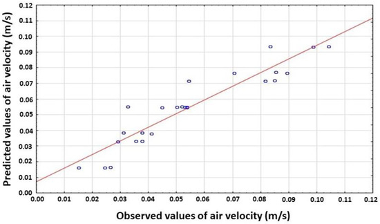
Figure 17.
Predicted versus observed values of air velocity in the reaction cell with lateral air inlet and outlet geometry.
Figure 18 illustrates the 2D response surface graphs of the interactive effects of statistically significant variables on velocity for this geometry. In particular, panels (a) and (b) point out an increase in velocity with the increase in air flow rate, which reveals that this parameter had the most important effect. However, the most significant values of the distances of air inlet and outlet were, in this case, the ones corresponding to the highest and lowest levels, respectively. This antagonism, which indeed was expected for these analyses, is confirmed in panel (c).
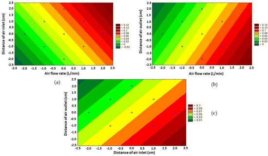
Figure 18.
2D contour graph of the interaction effects for the lateral air inlet and outlet geometry. Simultaneous effects on velocity exerted by (a) distance of air inlet and air flow rate; (b) distance of air outlet and air flow rate; (c) distance of air inlet and distance of air outlet.
Similarly, Table 10 lists the results of ANOVA applied to the internal pressure in the reaction cell for the same geometry, which was performed with a 95% confidence level. The p-values reveal the statistical significance of the linear and quadratic effects of air flow rate as well as that of the interaction between distances of air inlet and outlet, the first of them being the most impactful.
Table 10.
Results of the analysis of variance applied to the internal pressure in the reaction cell with lateral air inlet and outlet geometry.
Equation (7) represents the mathematical model found for internal pressure (P) in the reaction cell with this geometry including the statistically significant effects (
while Figure 19 displays the graph of predicted versus observed values. The excellent fit to the experimental data observed in this case, with a few residuals quite close to the line, confirms the accuracy of the model.
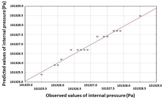
Figure 19.
Predicted versus observed values of internal pressure in the reaction cell with lateral air inlet and outlet geometry.
Similarly to what was performed for the other geometry, Figure 20 illustrates the 2D response surface graphs of the effects of the statistically significant variables on internal pressure for the geometry with lateral air inlet and outlet. Panels (a) and (b) show quite similar characteristics. An increase in pressure, albeit discrete, was found with the increase in air flow rate, and the effect of distance was even more discrete. The graph was generated setting the distance of the air outlet at level +1. Panel (c) shows a tendency toward a small increase in pressure when both distances are at levels +1, −1 or −1, +1 due to the term with the negative sign (Equation (7)). The graph was generated setting the air flow rate level at zero.
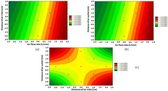
Figure 20.
2D contour graph of the interaction effects for the lateral air inlet and outlet geometry. Simultaneous effects on internal pressure exerted by (a) distance of air inlet and air flow rate; (b) distance of air outlet and air flow rate; (c) distance of air inlet and distance of air outlet.
3.3.2. Geometry with Upper Air Inlet and Outlet
The results gathered in the ANOVA table (Table 11) for air velocity in the reaction cell with upper air inlet and outlet geometry point out the statistical significance of the linear effects of air flow rate, reaction cell diameter, and distance of air inlet as well as the combination of reaction cell diameter and distance of air inlet.
Table 11.
Results of the analysis of variance applied to the air velocity in the reaction cell with upper air inlet and outlet geometry.
The mathematical model of V in the reaction cell with this geometry accounting for the statistically significant effects () is described by the equation:
while Figure 21 depicts the graph of predicted versus observed values of this response. A satisfactory fit to the experimental data was found, despite a slight dispersion close to the line.
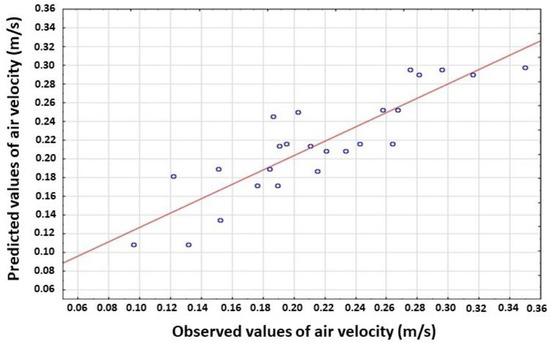
Figure 21.
Predicted versus observed values of air velocity in the reaction cell with upper air inlet and outlet geometry.
Figure 22 shows the 2D response surface graphs of the interactive effects of statistically significant variables on velocity for this geometry. Panel (a) points out an increase in velocity with the increase in air flow rate. Moreover, a slight increase in velocity was found with the reduction in the diameter of the reaction cell. Panel (b) shows an increase in velocity with the increase in air flow rate as well as a slight increase in velocity with the increase in the distance of the air inlet. Panel (c), which illustrates the combined effect of both distances, reveals a tendency toward a slight increase in velocity when they are at levels +1, +1 or −1, −1 due to the term with the positive sign (Equation (8)). The graph was generated setting the air flow rate level at 0.
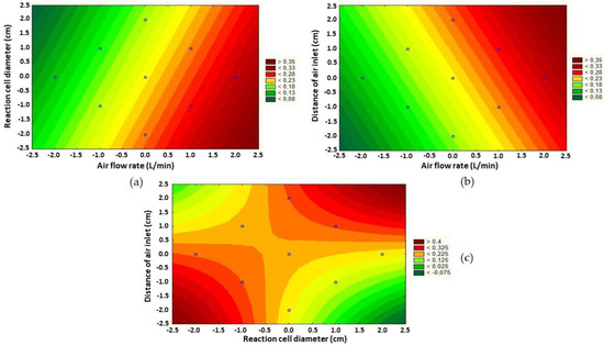
Figure 22.
2D contour graph of interaction effects for the upper air inlet and outlet geometry. Simultaneous effects on velocity exerted by (a) reaction cell diameter and air flow rate; (b) distance of air inlet and air flow rate; (c) distance of air inlet and reaction cell diameter.
Table 12 lists the ANOVA results regarding the internal pressure in the reaction cell for the same geometry. The p-values with a 95% confidence level revealed statistically significant effects of air flow rate (both linear and quadratic effects) and reaction cell diameter as well as of interaction between air flow rate (linear) and reaction cell diameter.
Table 12.
Results of the analysis of variance applied to the internal pressure in the reaction cell with upper air inlet and outlet geometry.
Equation (9) represents the mathematical model found for P in the reaction cell with this geometry considering the statistically significant effects ():
while Figure 23 displays the graph of predicted versus observed values of this response. The fit was excellent since all the points fell basically on the line almost without residuals, thereby confirming the reliability of the results obtained.
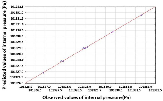
Figure 23.
Predicted versus observed values of internal pressure in the reaction cell with upper air inlet and outlet geometry.
Finally, Figure 24 illustrates the 2D response surface graph of the interactive effects of the statistically significant variables on internal pressure for this geometry. Air flow rate was the most impacting factor, in that its increase is associated with an increase in pressure. In contrast, pressure was practically the same regardless of the reaction cell diameter.
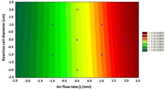
Figure 24.
2D contour graph of interaction effects of reaction cell diameter and air flow rate on the internal pressure for the upper air inlet and outlet geometry.
4. Discussion
4.1. Mesh Convergence Study
Flow Simulation considers the real model created in SOLIDWORKS and automatically generates a rectangular computational mesh in the computational domain distinguishing fluid and solid domains. In the meshing process, the computational domain is divided into uniform rectangular cells of parallelepiped shape that form the basic mesh. Using information on the geometry of the model, the contour conditions, and the specified objectives, Flow Simulation then constructs the mesh further through various refinements (division of the cells of the basic mesh into smaller cells), thus providing a better representation of the model and regions of the fluid. The initial mesh is defined by the basic mesh and refinement configurations [27].
In the study by Hoiberg and Shah [28], the velocity component was selected for the convergence study, as its magnitude was significantly greater than that of the other components and had a significant impact on sedimentation. According to Martins et al. [29], the most efficient meshes are those that meet two criteria: maximum precision and minimum computational effort, i.e., less CPU time.
Hoiberg and Shah [28] investigated the independence of the mesh by simulating it on three levels. The quantitative predictions were in strict agreement, with discrepancies of approximately 10%. Thus, the results were considered sufficiently independent, and the geometry with approximately 1.5 million cells was used in the simulation.
Palanisamy and Ayalur [25] found less than 5% variation in the parameters analyzed between refinement levels 5 and 6, with total cell counts of 2,280,800 and 4,820,487.
Serra and Semiao [30] analyzed the CPU time and number of cells necessary for convergence in the most efficient scenario of the study and achieved improvements ranging from 1 to 39% fewer iterations and 10 and 185% shorter CPU time in comparison to the other variables studied.
According to SolidWorks [27], if the estimated ratios are not too large, creating the mesh with the configurations of the standard mesh (automatic) is recommended, beginning with global mesh level 3 if the geometry of the model and flow field are relatively smooth, whereas mesh level 4 or 5 is recommended for more complex problems.
4.2. Results of CFD Simulation of Velocity and Pressure
Minto et al. [31] developed a field-scale reactive transport model in OpenFOAM CFD software for microbially induced carbonate precipitation (MICP) that captures the key processes of bacteria transport and attachment, urea hydrolysis, tractable CaCO3 precipitation, and modification of the porous media in terms of porosity and permeability. The results of this model, which was named biogroutFoam, pointed out the need to model bacterial adhesion as a function of fluid velocity and suggested that the adoption of phased injection strategies can lead to uniform precipitation in a porous medium.
In the CFD simulations performed by Zand and Saidi [32], the use of secondary jet inlets in regular spouted beds was effective in regulating the volume of air in the annulus, which conventionally has insufficient air flow rate. According to the built geometries, the fraction of air volume was doubled, at least in configurations with high velocity of the injection gas.
Ambedkar and Dutta [33] simulated a vortex tube with five types of inert gas to understand the influence of different properties of these gases on flow phenomena and thermal performance of the vortex tube in broad ranges of cold mass fraction and inlet pressure. Even though the nature of the contour of the axial velocity was similar for all gases, the magnitude of axial velocity strongly depended on the gas molar mass, and the gas density increased with the increase in molar mass. This diminished the magnitude of the axial velocity of the gas within the vortex tube to follow the conservation of momentum.
Jing et al. [34] found that static pressure profiles of the wall in a Venturi tube had a descending tendency in the convergent section under different conditions, with a faster reduction in pressure closer to the throat section. Moreover, the pressure on the wall increased gradually in the divergent section, but the outlet pressure was still lower than the inlet one. The same authors also reported that when a wet gas flows through the Venturi tube, the pressure diminishes and the flow velocity increases in the convergent section, and this tendency continues until the throat section reaches the peak. This process is in line with Bernoulli’s principle, by way of which Thompson and Hardy [35] stated that the pressure or the sum of kinetic energies and potential of a fluid current moving through a tube is constant. If the gas moves with laminar flow, the kinetic energy of the fluid increases as it moves through a constriction in a tube; therefore, the potential energy should drop according to the law of conservation of energy in order to maintain the total sum of energy constant.
In fluid mechanics, current lines are the trajectories of imaginary particles suspended in and transported by the fluid. With permanent flow, the fluid is in movement, but the current lines are fixed and instantaneously tangent to the flow velocity vector [36].
4.3. Statistical Analysis of Results of Velocity and Pressure Obtained in a Specific Region
Hadibafekr et al. [37] developed a study in which 25 CFD experiments were designed by central composite design (CCD) and conducted in a wavy lobed heat exchanger. Appropriate regression models for objective functions, i.e., Nusselt number ratio, friction factor ratio, performance evaluation criteria, and entropy generation number, were examined using statistical tools. According to the ANOVA results, the R2 of the reduced models was between 94.82% and 98.37%, indicating an acceptable precision of the models.
Carrero et al. [38] evaluated the mechanical properties of self-healing styrene-butadiene rubber compounds reinforced with ground tire rubber (GTR), where the influence of the microstructural GTR characteristics on the mechanical performance was studied through a statistical analysis based on the design of experiments methodology. Due to the complexity of the study, two full factorials were designed. It was possible to establish that decreasing network density and its interactions with surface area and filler amount were statistically significant for the tensile strength. The p-value obtained was less than 0.05, while R2 exceeded 98% under all the conditions studied, which demonstrates the reliability of the factorial response.
Lysova et al. [39] carried out a study on the behavior of a countercurrent tube-in-tube heat exchanger for fluid foods and simulated it under different operating conditions using CFD. Three independent variables (product velocity, inlet product temperature, and inlet water temperature) and two responses (outlet product temperature and pressure drop across the heat exchanger) were chosen, the selected product being a water suspension of 0.1% (w/w) gellan gum powder. Statistical analyses were performed on the results of both responses predicted by CFD simulations, and ANOVA was performed to determine whether the model and its terms were statistically significant (p-value < 0.05). For both estimated responses, the quadratic model and all its terms were significant, except for the product of the two input temperatures, and the values very close to 1, thus demonstrating its very good predicting performance. The pressure drop was influenced mainly by the product velocity, whereas product and water temperatures exerted a lower impact. The strongest positive effect on the inlet product temperature was exerted by water temperature, whereas an increase in product velocity led to a lower increase in product temperature, as the fluid residence time within the heat exchanger was reduced.
Yu et al. [40] carried out a study with the objective of designing and optimizing a new constructal regenerator with annular bifurcation to reduce the flow and axial losses by heat conduction in the regenerator using CFD and design of experiments. To further validate the accuracy of the quadratic polynomial regression models, the authors made comparisons between actual and predicted numerical values, and the points were shown to be uniformly distributed around the diagonal line. Since the mean deviations between predicted and actual values were only 9.7% and 8.2% for global friction factor and number of heat transfer units, respectively, they concluded, resorting to ANOVA, that the regression model was sufficiently accurate to predict the performance of the regenerator.
Zhang et al. [41] carried out a parametric evaluation of the main characteristics of a geometric design for a pressure relief valve (PRV) with a back pressure chamber and two adjustment rings. The work was conducted using CFD to model the dynamic performance of the opening and closing of a nuclear power main steam pressure relief valve (NPMS PRV), while a CCD and response surface methodology (RSM) were used to evaluate the effect of the position of adjustment elements on the discharge. The values predicted by the model equation for blowdown proved to be in satisfactory agreement with the observed ones, indicating that the developed regression quadratic models can be used to precisely estimate the factors of response for any variable that is in the numerical design range. This agreement was also confirmed by the adequate precision (AP) value (> 4) for the blowdown response. Therefore, it was possible to verify that the predicted model can be used to navigate the design space defined by the CCD procedure.
5. Conclusions
In the present work, simulations with computational fluid dynamics and experimental planning were used to optimize the geometry of a reaction cell in a cement biomineralization process. The effects of air flow, reaction cell diameter, distance of air inlet and outlet on air velocity, and internal pressure in the cell were investigated. The following conclusions can be drawn from the present study:
- The mesh convergence study gave reliable results, providing efficient meshes with maximum precision and minimum computational effort. Global mesh 4 and local mesh 5 were defined as the most adequate for all the runs.
- The results of simulations using computational fluid dynamics in the reaction cell revealed that air flow rate had the strongest positive impact on the air velocity. On the other hand, the internal pressure in the reaction cell varied little and remained close to ambient pressure, which was expected as temperature and pressure were constant.
- In the statistical analyses for the geometry with the lateral air inlet and outlet, a certain mirroring in the factors was found for air velocity and internal pressure, as the statistically significant effects were those of air flow rate, distance of air inlet, and distance of air outlet. Air flow rate was the main factor, since its increase led to an increase in velocity, corroborating the previous analyses. In contrast, reaction cell diameter had no statistically significant effect.
- The statistical analyses for the geometry with the upper air inlet and outlet also revealed that air flow rate was the main factor for both air velocity and internal pressure, with an increase in velocity resulting from the increase in air flow rate, corroborating the previous analyses. Moreover, reaction cell diameter and distance of air inlet also had a statistically significant effect on air velocity.
- Finally, in view of the data studied and according to the statistical analyses carried out, the most suitable reaction cell configuration for future applications in the cascade system for biomineralization in cement is the one with the air inlet and outlet in the lateral region. This geometry model has been selected as the most appropriate thanks to the repetition of statistically significant effects of air flow rate and distance of air inlet and outlet on the two studied responses, i.e., the air velocity and the internal pressure in the reaction cell. In this case, it would be possible to preserve the cell size, for instance, the diameter of air injection pipes as well as the reaction cell entrance and exit, by simply allocating them laterally. As this change would not require any increase in cell size, being just a position change, no additional cost to the project would be expected. In contrast, since the diameter had a statistically significant effect on the geometry with the air inlet and outlet in the upper region, the variation of this factor would imply a cost increase.
Supplementary Materials
The following supporting information can be downloaded at: https://www.mdpi.com/article/10.3390/en16083597/s1, Figures S1–S48: Air flow rate velocity in the reaction cell and streamlines; Figures S49–S96: Internal pressure in the reaction cell and the streamlines.
Author Contributions
Conceptualization, B.A.C.R.; methodology, B.A.C.R. and P.P.F.B.; formal analysis, B.A.C.R.; investigation, B.A.C.R.; resources, L.A.S.; data curation, B.A.C.R.; writing—original draft preparation, B.A.C.R., P.P.F.B., M.B. and L.A.S.; writing—review and editing, B.A.C.R., P.P.F.B., H.J.B.d.L.F., A.C., B.A., M.B. and L.A.S.; visualization, B.A.C.R.; supervision, M.B. and L.A.S.; project administration, Y.B.B., M.B. and L.A.S.; funding acquisition, A.C., B.A., M.B. and L.A.S. All authors have read and agreed to the published version of the manuscript.
Funding
The study was conducted with financial support to the research project from the Coordenação de Aperfeiçoamento de Pessoal de Nível Superior (CAPES [Coordination for Advancement of Higher Education Personnel]—Financial Code: 001), Universidade Federal de Pernambuco and Instituto Avançado de Tecnologia e Inovação (IATI [Advanced Institute of Technology and Innovation]), and with the assistance of the team of the Bioengineering Lab of Universidade Católica de Pernambuco (UNICAP). The authors are also grateful to Conselho Nacional de Desenvolvimento Científico e Tecnológico (CNPq [National Council of Scientific and Technological Development]).
Data Availability Statement
The data presented in this study are available on request from the corresponding author. The data are not publicly available due to privacy restrictions.
Acknowledgments
This work was developed as part of a thesis to be presented to the Programa de Pós-Graduação em Engenharia Química (PPGEQ [Postgraduate Program in Chemical Engineering]) of Universidade Federal de Pernambuco (UFPE).
Conflicts of Interest
The authors declare no conflict of interest. The funders had no role in the design of the study; in the collection, analyses, or interpretation of data; in the writing of the manuscript; or in the decision to publish the results.
References
- Wasim, M.; Abadel, A.; Bakar, A.; Alshaikh, I.M.H. Future directions for the application of zero carbon concrete in civil engineering—A review. Case Stud. Constr. Mater. 2022, 17, e01318. [Google Scholar] [CrossRef]
- Das, S.; Saha, P.; Jena, S.P.; Panda, P. Geopolymer concrete: Sustainable green concrete for reduced greenhouse gas emission–A review. Mater. Today Proc. 2022, 60, 62–71. [Google Scholar] [CrossRef]
- Ahmad, J.; Zhou, Z. Mechanical properties of natural as well as synthetic fiber reinforced concrete: A review. Constr. Build. Mater. 2022, 333, 127353. [Google Scholar] [CrossRef]
- Mauludin, L.M.; Oucifj, C. Modeling of Self-Healing Concrete: A Review. J. Appl. Comput. Mech. 2019, 5, 526–539. [Google Scholar] [CrossRef]
- Algaifi, H.A.; Bakar, S.A.; Sam, A.R.M.; Ismail, M.; Abidin, A.R.Z.; Shahir, S.; Altowayti, W.A.H. Insight into the role of microbial calcium carbonate and the factors involved in self-healing concrete. Constr. Build. Mater. 2020, 254, 119258. [Google Scholar] [CrossRef]
- Ruan, S.; Qiu, J.; Weng, Y.; Yang, Y.; Yang, E.; Chu, J.; Unluer, C. The use of microbial induced carbonate precipitation in healing cracks within reactive magnesia cement-based blends. Cem. Concr. Res. 2019, 115, 176–188. [Google Scholar] [CrossRef]
- Nguyen, T.H.; Ghorbel, E.; Fares, H.; Cousture, A. Bacterial self-healing of concrete and durability assessment. Cem. Concr. Compos. 2019, 104, 103340. [Google Scholar] [CrossRef]
- Roque, B.A.C.; Brasileiro, P.P.F.; Brandão, Y.B.; Casazza, A.A.; Converti, A.; Benachour, M.; Sarubbo, L.A. Self-healing Concrete: Concepts, Energy Saving and Sustainability. Energies 2023, 16, 1650. [Google Scholar] [CrossRef]
- Brasileiro, P.P.F.; Brandao, Y.B.; Sarubbo, L.A.; Benachour, M. Self-Healing Concrete: Background, Development, and Market Prospects. Biointerface Res. Appl. Chem. 2021, 11, 14709–14725. [Google Scholar] [CrossRef]
- Gao, Z.; Liu, H.; Xu, X.; Xiahou, X.; Cui, P.; Mao, P. Research Progress on Carbon Emissions of Public Buildings: A Visual Analysis and Review. Buildings 2023, 13, 677. [Google Scholar] [CrossRef]
- Zhu, W.; Huang, B.; Zhao, J.; Chen, X.; Sun, C. Impacts on the embodied carbon emissions in China’s building sector and its related energy-intensive industries from energy-saving technologies perspective: A dynamic CGE analysis. Energy Build. 2023, 287, 112926. [Google Scholar] [CrossRef]
- Zhang, M.; Yang, D.; Du, J.; Sun, H.; Li, L.; Wang, L.; Wang, K. A Review of SOH Prediction of Li-Ion Batteries Based on Data-Driven Algorithms. Energies 2023, 16, 3167. [Google Scholar] [CrossRef]
- Seifan, M.; Samani, A.K.; Berenjian, A. New insights into the role of pH and aeration in the bacterial production of calcium carbonate (CaCO3). Appl. Microbiol. Biotechnol. 2017, 101, 3131–3142. [Google Scholar] [CrossRef] [PubMed]
- Jankovic, A.; Chaudhary, G.; Goia, F. Designing the design of experiments (DOE)–An investigation on the influence of different factorial designs on the characterization of complex systems. Energy Build. 2021, 250, 111298. [Google Scholar] [CrossRef]
- Lee, B.C.Y.; Mahtab, M.S.; Neo, T.H.; Farooqi, I.H.; Khursheed, A. A comprehensive review of Design of experiment (DOE) for water and wastewater treatment application—Key concepts, methodology and contextualized application. J. Water Process. Eng. 2022, 47, 102673. [Google Scholar] [CrossRef]
- Chen, F.; Zhu, G.; Yao, B.; Guo, W.; Xu, T. Sand-ejecting fire extinguisher parameter sensitivity analysis based on DOE and CFD-DEM coupling simulations. Adv. Powder Technol. 2022, 33, 103719. [Google Scholar] [CrossRef]
- Venkatesan, L.; Harris, A.; Greyling, M. Optimisation of air rate and froth depth in flotation using a CCRD factorial design–PGM case study. Miner. Eng. 2014, 66–68, 221–229. [Google Scholar] [CrossRef]
- Shen, R.; Jiao, Z.; Parker, T.; Sun, Y.; Wang, Q. Recent application of Computational Fluid Dynamics (CFD) in process safety and loss prevention: A review. J. Loss Prev. Process Ind. 2020, 67, 104252. [Google Scholar] [CrossRef]
- Bournet, P.-E.; Rojano, F. Advances of Computational Fluid Dynamics (CFD) applications in agricultural building modelling: Research, applications and challenges. Comput. Electron. Agric. 2022, 201, 107277. [Google Scholar] [CrossRef]
- Lins, I.X.; Filho, H.J.B.L.; Santos, V.A.; Pereira, J.C.S.; Mak, J.; Vieira, C.W. Hydrodynamic study of the oil flow in a protective relay coupled to a power transformer: CFD simulation and experimental validation. Eng. Fail. Anal. 2021, 128, 105599. [Google Scholar] [CrossRef]
- Zhang, R.; Zhang, Y.; Lam, K.P.; Archer, D.H. A prototype mesh generation tool for CFD simulations in architecture domain. Build. Environ. 2010, 45, 2253–2262. [Google Scholar] [CrossRef]
- Yu, F.; Zhang, H.; Li, Y.; Xiao, J.; Class, A.; Jordan, T. Voxelization-based highefficiency mesh generation method for parallel CFD code GASFLOW-MPI. Ann. Nucl. Energy 2018, 117, 277–289. [Google Scholar] [CrossRef]
- Brasileiro, P.P.F.; Roque, B.A.C.; Bradão, B.Y.; Casazza, A.A.; Converti, A.; Benachour, M.; Sarubbo, L.A. Cascade system for biomineralization in cement: Project, construction and operationalization to enhance building energy efficiency. Energies 2022, 15, 5262. [Google Scholar] [CrossRef]
- Rodrigues, M.I.; Iemma, A.F. Planejamento de Experimentos & Otimização de Processos, 3rd ed.; Cárita Editora: Campinas, Brazil, 2014; p. 358. [Google Scholar]
- Palanisamy, D.; Ayalur, B.K. Impact of condensate cooled air purging on indoor air quality in an air conditioned laboratory. Build. Environ. 2021, 188, 107511. [Google Scholar] [CrossRef]
- Botan, A.C.B. Otimização de um Modelo de Turbina Hidráulica Tipo Bulbo Aplicada em Condições de Queda Ultrabaixa. Ph.D. Thesis, Universidade Federal de Itajubá, Itajubá, Brazil, 2019. [Google Scholar]
- SolidWorks. Technical Reference Solidworks Flow Simulation 2020; Dassault Systems: Waltham, MA, USA, 2020. [Google Scholar]
- Hoiberg, B.; Shah, M.T. CFD study of multiphase flow in aerated grit tank. J. Water Process. Eng. 2021, 39, 101698. [Google Scholar] [CrossRef]
- Martins, N.M.C.; Carriço, N.J.G.; Ramos, H.M.; Covas, D.I.C. Velocity-distribution in pressurized pipe flow using CFD: Accuracyand mesh analysis. Comput. Fluids 2014, 105, 218–230. [Google Scholar] [CrossRef]
- Serra, N.; Semiao, V. ESIMPLE, a new pressure–velocity coupling algorithm for built-environment CFD simulations. Build. Environ. 2021, 204, 108170. [Google Scholar] [CrossRef]
- Minto, J.M.; Lunn, R.J.; El Mountassir, G. Development of a reactive transport model for field-scale simulation of microbiallyinduced carbonate precipitation. Water Resour. Res. 2019, 55, 7229–7245. [Google Scholar] [CrossRef]
- Zand, M.K.; Saidi, M. Numerical investigation of lateral aeration effect on gas-solid flow and particle mixing in spouted bed with different base angles. Powder Technol. 2022, 412, 117924. [Google Scholar] [CrossRef]
- Ambedkar, P.; Dutta, T. CFD simulation and thermodynamic analysis of energy separation in vortex tube using different inert gases at different inlet pressures and cold mass fractions. Energy 2023, 263, 125797. [Google Scholar] [CrossRef]
- Jing, J.; Yuan, Y.; Du, S.; Yin, X.; Yin, R. A CFD study of wet gas metering over-reading model under high pressure. Flow Meas. Instrum. 2019, 69, 101608. [Google Scholar] [CrossRef]
- Thompson, N.; Hardy, L. Physics of gases. Anaesth. Intensive Care Med. 2021, 22, 33–36. [Google Scholar] [CrossRef]
- Alhajahmad, A.; Mittelstedt, C. A novel grid-stiffening concept for locally reinforcing window openings of composite fuselage panels using streamline stiffeners. Thin Walled Struct. 2022, 179, 109731. [Google Scholar] [CrossRef]
- Hadibafekr, S.; Mirzaee, I.; Khalilian, M.; Shirvani, H. Thermo-entropic analysis and multi-objective optimization of wavy lobed heat exchanger tube using DOE, RSM, and NSGA II algorithm. Int. J. Therm. Sci. 2023, 184, 107921. [Google Scholar] [CrossRef]
- Carrero, K.C.N.; Pastor, L.E.A.; Santana, M.H.; Pastor, J.M. Design of self-healing styrene-butadiene rubber compounds with ground tire rubber-based reinforcing additives by means of DoE methodology. Mater. Des. 2022, 221, 110909. [Google Scholar] [CrossRef]
- Lysova, N.; Solari, F.; Vignali, G. Optimization of an indirect heating process for food fluids through the combined use of CFD and Response Surface Methodology. Food Bioprod. Process. 2022, 131, 60–76. [Google Scholar] [CrossRef]
- Yu, M.; Shi, C.; Liu, Z.; Liu, W. Design and multi-objective optimization of a new annular constructal bifurcation Stirling regenerator using response surface methodology. J. Heat Mass Transf. 2022, 195, 123129. [Google Scholar] [CrossRef]
- Zhang, J.; Yang, L.; Dempster, W.; Yu, X.; Jia, J.; Tu, S.-T. Prediction of blowdown of a pressure relief valve using response surface methodology and CFD techniques. Appl. Therm. Eng. 2018, 133, 713–726. [Google Scholar] [CrossRef]
Disclaimer/Publisher’s Note: The statements, opinions and data contained in all publications are solely those of the individual author(s) and contributor(s) and not of MDPI and/or the editor(s). MDPI and/or the editor(s) disclaim responsibility for any injury to people or property resulting from any ideas, methods, instructions or products referred to in the content. |
© 2023 by the authors. Licensee MDPI, Basel, Switzerland. This article is an open access article distributed under the terms and conditions of the Creative Commons Attribution (CC BY) license (https://creativecommons.org/licenses/by/4.0/).