Abstract
This paper is related to light pollution and the energy efficiency of outdoor amenity lighting. It concerns the standard design assessment parameters of light pollution, the Upward Light Ratio (ULR) and Upward Flux Ratio (UFR), and the classic energy efficiency parameter—Normalized Power Density (NPD). The motivation for this research was the observation of certain inaccuracies related to the applicability and interpretation of these parameters in practice and the lack of connection between parameters of light pollution and energy efficiency. The multi-variant computer simulations of the exemplary large-area parking lot lighting system were conducted. Over four hundred cases were carefully analyzed. Individual cases differ in the shape of the task area, luminaire arrangements, mounting height, luminous intensity distribution, aiming, and maintenance factor. The results confirmed that the criteria values of ULR and UFR are often overestimated for modern luminaires, which emit luminous flux emitted only downwards. In this case, the ULR and UFR values do not exceed the criteria values for even zones with lower ambient brightness. Thus, lighting solutions with much lower energy efficiency easily meet the requirements of these parameters. This situation is not rational. So, it is crucial to make the criteria of ULR and UFR much more stringent in all environmental zones. Moreover, the research confirms a strong positive linear correlation between UFR and NPD (0.92, p < 0.001), which means that light pollution can be reduced by ensuring an appropriate level of energy efficiency. It is a great help in designing sustainable outdoor amenity lighting.
1. Introduction
Light pollution is an issue that scientists and engineers around the world have studied for at least 30 years. In the literature, many works presenting various essential aspects of this phenomenon can be found. The influence of light pollution on changes in the broadly understood natural environment is analyzed the most frequently nowadays. The works mainly concern the impact of lighting on living organisms. Research is carried out to show how light pollution affects the population and functioning of various species of insects, birds, and bats [1,2,3,4,5,6].
Another group of works is related to astronomical issues [7,8,9,10,11]. One of the disadvantages of light pollution is the formation of skyglow. It causes the night sky, which should be dark, to be brightened. As a result, many celestial bodies are impossible to observe, and the work of people engaged in astronomy is difficult or even impossible to perform (Figure 1A) [10,12]. Additionally, there was some difference in the definition of surface brightness by engineers and astronomers. Therefore, some works also concern the derivation of appropriate mathematical formulas enabling the transition from the luminance scale to the magnitude scale, taking into account the luminous efficiency function of human vision [13].
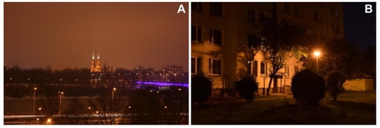
Figure 1.
Examples of light pollution consequences: (A)—the lack of stars’ visibility over the city of Warsaw due to skyglow, (B)—obtrusive light (light intrusion) into the residential building (both photos: K. Skarżyński).
Many of the papers relate to measurement techniques and light pollution monitoring. Appropriate hardware solutions are created, and sometimes they are combined into entire measurement networks that enable the analysis of the surface brightness of the night sky [14,15]. The influence of weather conditions on the obtained results is also analyzed [16]. There is also great interest in using unmanned aerial vehicles to inspect light pollution in a given area quickly [17,18]. Moreover, the interest is also given in analyzing luminance distribution on a night sky, building surfaces, or lighting equipment using luminance cameras [19,20,21,22].
In the works related to light pollution, one can also analyze its impact on electricity consumption, general economic issues, civilization development, and human well-being [23,24,25,26,27]. Exposure to light at night can cause circadian rhythm disturbances in humans and animals [28]. In cities, a widespread phenomenon is light trespassing into the interiors of buildings (Figure 1B), which irritates their users [29]. However, the awareness of this problem is not high enough [30,31,32]. Selected papers are also devoted to more technical issues related to the lighting design process to obtain an optimal and sustainable solution for various types of lighting installation, including even interior lighting [33,34,35,36,37,38,39].
It can be easily observed that the problem of light pollution is critical and widely analyzed in many aspects. Its main cause is the use of various electric lighting installations at night. However, not all outdoor lighting installations are correctly designed and implemented to minimize light pollution and maximize energy efficiency. This problem of light pollution is so severe that some countries have also decided to tighten the requirements related to light pollution to reduce it [40,41]. There are associations whose main task is protecting the dark sky, e.g., the International Dark-Sky Association [42]. Technical committees within the International Commission on Illumination (CIE) also work to address light pollution problems. These organizations and groups defined a general framework by which light pollution can be reduced. Lighting installations must be useful, be adequately targeted, realize low brightness levels, be controllable, and the appropriate spectral power distributions (especially for LED equipment) must be selected. So, the acceptability of light pollution of a given lighting installation concerning skyglow can be determined based on appropriate quantitative parameters, e.g., the Upward Light Ratio (ULR) and Upward Flux Ratio (UFR) or luminous intensity limitations in individual angles above the horizon [43,44]. However, the literature needs a thorough analysis of the criteria values of these parameters concerning the state of the art of the currently used lighting equipment and the lighting design process. Therefore, the main goal of this paper is to present the authors’ considerations about the applicability of the ULR and UFR parameters in design practice and study the relation between light pollution and energy efficiency parameters for outdoor amenity lighting.
2. Upward Light Ratio and Upward Flux Ratio
A typical situation in outdoor lighting is shown in Figure 2. Part of the luminous flux from the lighting system can be directly emitted into the upper hemisphere. Some components may reach the task field, some may reach the surroundings, and some may be reflected. The described situation is the simplest case and does not consider other objects that may be present in the vicinity of, e.g., residential buildings. However, on its basis, it is possible to define some quantitative parameters for assessing light pollution related to the emission of the luminous flux into the upper hemisphere: the Upward Light Ratio (1) and Upward Flux Ratio. (2–3). A brief definition of these parameters is presented below.
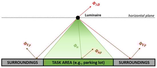
Figure 2.
The scheme of the basic and typical situation of outdoor amenity lighting:
—luminous flux directly emitted into upper hemisphere, —useful luminous flux, —luminous flux reflected from the task area, and —luminous flux reflected from surroundings.
Upward Light Ratio (ULR): It is the ratio of the luminous flux of luminaires emitted directly into the upper hemisphere (above the horizon) and the total luminous flux of these luminaires (1).
where:
- is the upward light ratio [%]
- is the luminous flux emitted directly into the upper hemisphere [lm]
- is the total luminous flux of all luminaires used [lm]
Upward Flux Ratio (UFR): While the ULR only considers the luminous flux of the luminaires emitted directly upwards, the UFR also considers the luminous flux reflected upwards from the substrate, both from the area intended for illumination (task area) and the area that is not (surroundings). The basic UFR mathematical definition is presented by Formula (2). It is complex and can be found in “Guide on the Limitation of the Effects of Obtrusive Light from Outdoor Lighting Installations, 2nd edition” from 2017 [43]. However, it can be defined much more easily and adequately understood. The UFR is the ratio of the maximum luminous flux emitted upwards for a given lighting solution to the minimum value of the luminous flux emitted upwards in an ideal situation (3). The ideal situation should be understood as obtaining 100% of the utilization factor and the average illuminance value equal to the criterion value adopted based on the relevant lighting standard.
where:
- is the upward flux ratio [-]
- is the average maintained illuminance achieved in the given solution (design) [lx]
- is the average maintained illuminance required on the task area (from the lighting standard) [lx]
- is the maintenance factor [-]
- is the utilisation factor [%]
- is the upward light output ratio in given luminaires position [-]
- is the downward light output ratio in given luminaires position [-]
- is the reflectance of task area [-]
- is the reflectance of surroundings [-]
- is the maximum luminous flux emitted upwards in a given lighting solution [lm]
- is the minimum value of the luminous flux emitted upwards in an ideal situation [lm]
Examples of ULR and UFR criteria values for individual environmental zones are presented in Table 1. They were also taken from the above-mentioned CIE technical report no. 150 [43]. It is worth noting that in this paper the UFR criteria values were presented only for amenity lighting because only this type of lighting installation will be analyzed in the presented case study. The UFR criteria values for sport lighting and road lighting are different. Moreover, the calculation procedure of this parameter for road lighting is also slightly different, depending on the geometry of the illuminated road [43].

Table 1.
ULR and UFR criteria values in environmental zone for amenity lighting [43].
3. Material and Methods
3.1. Research Hypotheses
It is worth noting that UFR values present in Table 1 are very high for amenity lighting. In the E4 environmental zone, which is responsible for areas with high ambient brightness, e.g., city centers, its permissible value is 35. It means that the maximum allowable flux emitted into the upper half-space may be 35 times greater than the minimum resulting from the adopted design criteria. The currently used lighting equipment is mainly based on LED technology [45,46,47,48,49]. The luminaires usually emit 100% of their luminous flux only into the lower hemisphere, even when tilted. In addition, in the formula for UFR, there is a quantity called the utilization factor, which is the ratio between useful luminous flux that reaches the task area and total luminous flux from all light sources. This quantity directly impacts the energy efficiency performance of the designed solution as it is connected with classical assessment parameters such as Lighting Power Density and Normalized Power Density [44,50]. Therefore, there is no direct connection between light pollution and energy efficiency assessment parameters.
Considering the above information, the following two hypotheses of this research can be defined as follows:
- I.
- The UFR criterion values are too high, not adapted to the current capabilities of lighting equipment, and must be strictly lowered;
- II.
- There is a strong interplay between UFR and NPD. Therefore, the light pollution from amenity lighting installation can be assessed by the value of NPD.
3.2. Multi-Variant Simulation Studies
The research methods are based on the computer simulation of lighting using dedicated software. Therefore, the DIALux 4 was used as it is reliable for lighting calculations, and it is possible to quickly obtain the ULR value directly for a given lighting solution [51,52,53]. When analyzing the primary sources of light pollution in urban areas, it was determined that one of them is large-area parking lots [54,55]. The area for illumination in such a facility may be several thousand square meters. Therefore, it was decided to simulate the lighting for such an object with an area of 10,000 m2 in a variant approach. The highest requirements for the luminous environment for the parking lot have been adopted following the European standard for outdoor workplaces [56]. As these facilities are located in the urban zone (high ambient brightness), the requirements for the ULR and UFR parameters will be the same as in the environmental zone E4. Calculations of the UFR parameter were made assuming that the task field reflectance is the same as for the surroundings and is 20%. In addition, it was decided to analyze the obtained values of utilance instead of the utilization factor (4). It is because the utilance directly informs the designer how much luminous flux from the luminaires reaches the task area. Moreover, the normalized power density power was selected as an energy efficiency indicator (5).
Utilance is the ratio of the useful luminous flux reaching the task area and the total luminous flux of all used luminaires [44].
where:
- is the utilance [%]
- is the useful luminous flux [lm]
- is the total luminous flux of all luminaires used [lm]
Normalized Power Density (NPD) is the lighting power density related to the level of 100 lx. This parameter is a classic measure of energy efficiency for various types of lighting installations [50].
where:
- is the normalized power density [W/m2|100 lx]
- is the lighting power density [W/m2]
- is the average maintained illuminance achieved in the given solution (design) [lx]
As there are no formal requirements related to the values of these parameters for the lighting of parking lots, it was decided that the utilance should aim at one and the normalized power density to zero. The summary of the adopted all assumed requirements is presented in Table 2.
Table 2.
Settled requirements for particular parameters.
As mentioned earlier, the lighting simulations were carried out in a variant approach, assuming the following variables:
- ▪
- Two parking lots with the area of 10,000 m2: 100 m × 100 m and 50 m × 200 m;
- ▪
- Two arrangements of luminaires: poles located on the edges of the parking lot and the parking lot surface, and poles located only on the parking lot surface. In both cases, the arrangement of poles is even and symmetrical concerning the symmetry axis of the parking lot shape (Figure 3);
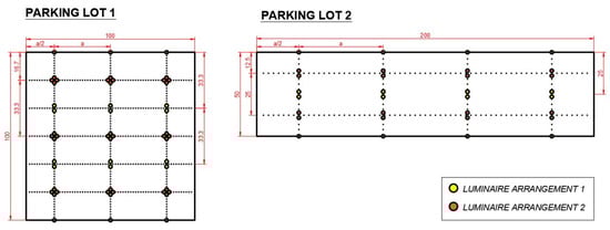 Figure 3. Schematic layout of poles on the area of analyzed parking lots.
 - ▪
- Six different types (A–F) of luminous intensity distributions of the LED luminaire with the same luminous flux of 10,000 lm (Figure 4). The active power of the luminaires is from 68 W to 76 W, corresponding with luminaire luminous efficacy of 147 lm/W and 132 lm/W, respectively;
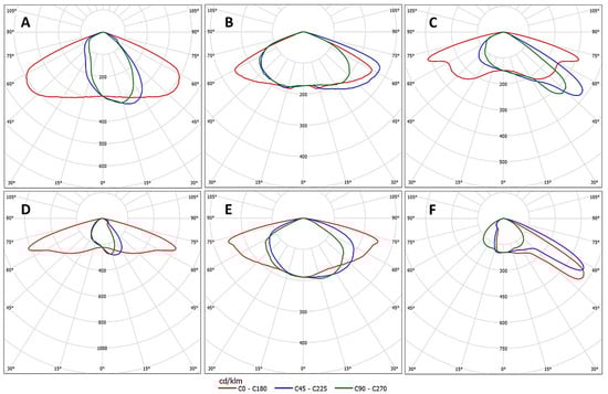 Figure 4. Luminous intensity distribution curves of the LED luminaire used (types (A–F)).
 - ▪
- Three tilts of the luminaires: 0°, 15°, 30°;
- ▪
- Three mounting heights of luminaires: 9 m, 12 m, and 15 m;
- ▪
- Two maintenance factors of 0.71 and 0.91 correspond to a relatively small (110%) and relatively large (140%) oversizing of lighting level.
Calculations of the luminous environment parameters were made following the European standard for outdoor lighting [56]. The dimension of the calculation grid is 4 m, and the calculation points have been evenly distributed over the area of both parking lots. In total, 432 lighting solutions were obtained for which all the previously discussed parameters of the luminous environment, light pollution, and energy efficiency were calculated. By analyzing such many cases and variables, it is possible to determine the relationship between the parameters of light pollution and energy efficiency. However, it should be noted that for significant changes in the assumptions (e.g., emission also into the upper hemisphere or other reflectance values of the task field and the surroundings), the obtained results will be different. Nevertheless, simulation studies identify the most typical solutions and everyday lighting situations. Then, the obtained results were compared, presenting histograms of the relevant parameters. Finally, we decided to investigate whether there is a linear correlation between the UFR parameter and the utilance and the normalized power density, and if so, what level it is.
4. Results and Discussion
In the beginning, the obtained results were analyzed to meet the normative requirements for the luminous environment. The results are shown in Figure 5. In 96% of cases, it was enough to use no more than 50 luminaires of a given type to illuminate an area as large as 10,000 m2. In 100% of cases, the value of the average maintained illuminance was obtained following the normative requirements (20 lx). The illuminance uniformity in 90% of cases exceeds the value of 0.25 and most often has a value from 0.30 to 0.50. Solutions with very high uniformity of over 0.5 (51 cases) were also obtained, corresponding to 12% of all cases. For 96% of all cases, the maximum value obtained in the calculation point of the glare (GR) is less than or equal to 50, which is a condition for meeting the normative requirements for this parameter. The GR values exceeding 50 are obtained for cases where the luminaires are installed in the lowest analyzed working position (9 m) and are tilted by 30°. This result aligns with the predictions based on the glare and design practice definition for outdoor workplaces [57,58,59].

Figure 5.
The histograms presenting the distribution of obtained results for: (A)—number of luminaires, (B)—average illuminance (including maintenance factor), (C)—uniformity of illuminance, and (D)—glare rating.
The distributions of the results of calculations of the ULR and UFR parameters are presented in Figure 6. For 360 cases (approx. 84% of all cases), the value of the ULR parameter does not exceed 2.5%, which means that these solutions meet the requirements for this parameter in the environmental zone E2. The ULR parameter for only 48 lighting solutions ranges from 5% to 15%. The maximum value obtained is 7.5%, linked to the luminaires’ tilt of 30°. It is worth emphasizing that in no case did the ULR value exceed 15%, and this means that all lighting solutions meet the requirements of the high-brightness environmental zone E4.
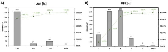
Figure 6.
The histograms presenting the distribution of obtained results for: (A)—Upward Light Ratio and (B)—Upward Flux Ratio.
Taking into account the obtained results of the UFR parameter, it should, first of all, be noted that the obtained values, even for extensive lighting oversize (140%, MF = 0.71) and large tilt of the luminaires, are lower than the requirements for zone E4. The UFR values are most often in the range of 2 to 4. Only in 13 cases of the obtained values exceed 5. This means that 97% of the cases meet the requirements for the E2 zone, and 100% are suitable for the E3 and E4 zones (Table 1). It is because, in all the luminaires used, the emission of the luminous flux occurs only and exclusively in the lower hemisphere. Relatively large tilts, even by 30°, causes the value of the UFR parameter increases. However, it does not exceed the requirements for zones with high ambient brightness (E4).
Figure 7 shows the distribution of the calculation results for the normalized power density. The lowest obtained value of this parameter is 0.81 W/m2|100 lx, while the highest is 2.42 W/m2|100 lx. It should be emphasized that higher values of NPD are most often associated with higher values of the UFR parameter. This observation aligns with the generally accepted assumption that light pollution is related to the energy efficiency issue.
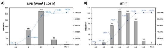
Figure 7.
The histograms presenting the distribution of obtained results for: (A)—Normalized Power Density and (B)—Utilance.
The histogram of the obtained values of the utilance is shown in Figure 8. Interestingly, in 369 cases, the value of this parameter is greater than or equal to 0.5. It means that 85% of all cases are characterized by 50% or more of the luminous flux of all luminaires reaching the task area. The distribution of the obtained lighting efficiency values resembles the normal distribution. Both weak cases in terms of luminaires’ luminous flux usage and those in which minimal losses can be distinguished. In the worst case, the utilance reached the value of 0.31. It was achieved with luminaires installed on poles with a height of 15 m and a tilt of 30°. In this case, the highest value of the UFR (7.5) and the normalized power density (2.42 W/m2|100 lx) were also obtained.
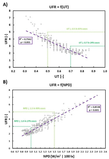
Figure 8.
The linear correlation between particular parameters: (A)—Upward Flux Ratio and Normalized Power Density, (B)—Upward Flux Ratio and Utilance.
In contrast, the case with the best luminous flux usage (utilance equals 0,86) was achieved for mounting the luminaires at 9 m and a tilt of 0°. In this case, the UFR is 2.35, and the normalized power density is 0.81 W/m2|100 lx. However, this case does not meet the requirements of a luminous environment because the uniformity value is 0.11. Thus, this lighting solution could only be implemented with the fair values of quantitative parameters related to light pollution and energy efficiency. It is also worth emphasizing that the parameter of utilance determines the engineering correctness of a given lighting solution. Therefore, to eliminate light pollution, it is recommended to analyze it at the design stage, during which one should strive to ensure that its value for a given lighting solution is close to 1. When a value close to 1 is obtained, it means that the total luminous flux of all luminaires reaches only and exclusively the area intended for the task area. However, this may not always be the best lighting solution due to light pollution. It also depends on the obtained oversizing lighting level, which is strongly connected with the adopted maintenance system. The designed lighting does not increase light pollution to a greater extent than the minimum, which is impossible to eliminate if the adopted value of the maintenance system is rational or if an appropriate control system is used. Therefore, based on the appropriate manufacturer’s datasheets, it is crucial to provide data on the luminous flux decrease of the luminaire (or source) during its operation and the reasonable determination of lighting equipment contamination possibility in a given location. The constant lumen output system (CLO) can also be valuable in providing the desired level of average maintained illuminance and avoiding oversizing, but such equipment can be costly. A good and less expensive solution is to use a control system that allows for manual or automatic switching off of the lighting system when no users are in the facility.
Because the highest UFR values correspond to both the highest NPD values and the lowest values of utilance, we decided to investigate the correlation between these parameters. The scatter plots of the relationships between UFR and NPD and the UFR and the utilance are presented in Figure 8. A trend line was determined for the obtained values based on linear regression for a given set. The value of the R2 parameter, which specifies the square of Pearson’s linear correlation coefficient, was also calculated. The obtained results determined that between the UFR parameter and the NPD, there is a strong positive linear correlation of 0.92 (with a significance level of p < 0.001). On the other hand, there was a strong negative linear correlation of −0.87 between the UFR and the utilance (with a significance level of p < 0.001).
Moreover, the results showed that in 81% of cases, the obtained UT value is at least 0.5 (50%), corresponding to a UFR value not higher than 5. For 24% of all cases, the UT is bigger than 0.7 (70%). For these cases, the UFR values are less than 3. A similar situation was obtained for the relationship between NDP and UFR. In 90% of cases, the obtained NPD value is at most 1.5 W/m2|100 lx, corresponding to the UFR value not higher than 5. For 27% of all cases, the NPD values do not exceed the 1.0 W/m2|100 lx, associated with UFR values less than 3. Therefore, it is possible to quantify the issue of light pollution from a given lighting installation based on the accurate calculation of NPD or utilance. However, it should be emphasized that the above discussion is done only for the luminaires whose luminous efficacy is approx. 140 lm/W. The long-observed tendency to increase luminous efficiency will undoubtedly contribute to reducing the value of the NPD and, as a result, may have a positive impact on the energy efficiency of lighting solutions. However, it requires proposing an adequate scale, including, e.g., additional analysis of typically used lighting equipment performance and determination of energy efficiency classes for outdoor amenity lighting.
5. Conclusions
This paper considers the interplay between light pollution and energy efficiency parameters. It describes the usefulness and applicability of parameters for the quantitative assessment of light pollution at the design stage—the Upward Light Ratio and Upward Flux Ratio. It could be achieved based on a variant lighting simulation of a typical outdoor lighting facility—a large city parking lot. The obtained results and the analysis proved the first hypotheses of this research. The prediction that the criteria values of the UFR parameters are too high in the case of amenity lighting and not adapted to the capabilities of the currently used standard lighting equipment is true. Therefore, making the requirements much stricter is necessary, e.g., the maximum value of UFR shall not exceed 3 in environmental zones E2–E4. However, it should be emphasized that the conducted research, despite the high number of cases, was limited to only one type of object. To accurately define the new criteria values of ULR and UFR, more cases should be analyzed in other outdoor lighting installations, such as sports and road lighting. It will be the basis for further research conducted by the authors of this article.
Finally, there are two critical observations. First, the UFR is very complicated, especially regarding its calculations. Not all commercial simulation programs commonly used can directly show the UFR value, but most of them can determine the NPD value. Or at least NPD is much easier to calculate than UFR. This research showed a strong positive correlation between UFR and NPD for outdoor amenity lighting. The higher NPD is, the higher UFR is. Therefore, the second hypothesis of this research was proven. So, an alternative approach to using the UFR parameter is to create an appropriate scale based on the normalized power density, which is easier to understand and more commonly used by engineers. Based on the presented research, the UFR value should not exceed 5 (or even 3). Moreover, NPD shall not exceed 1.0 W/m2|100 lx for using modern luminaires (luminous efficacy approx. 140 lm/W and light distribution only into the bottom hemisphere).
Additionally, to ensure that a given lighting installation is adequately designed, it is necessary to analyze the obtained utilance during the design process. This parameter can easily indicate if the luminous flux reaches the area that needs to be illuminated. In the design process of outdoor amenity lighting, high utilance values of at least 0.7 (70%) should be ensured, as they are related to the low value of the UFR.
Lastly, whether the criteria values of the parameters for the quantitative assessment of light pollution should be different in individual environmental zones (except for the E0 protection zone) should also be considered. Assigning an area to a given zone is problematic and may result in some unfair design practices or simple mistakes. From the view of engineering correctness, understood as the lack of intensification of light pollution and obtaining solutions with high energy efficiency, it seems that the requirements should be standardized regardless of where the illuminated object is located.
Author Contributions
Conceptualization, K.S.; methodology, K.S.; validation, K.S.; formal analysis, K.S. and A.R.; investigation, K.S. and A.R.; resources, K.S. and A.R.; data curation, K.S. and A.R; writing—original draft preparation, K.S.; writing—review and editing, K.S.; visualization, K.S.; supervision, K.S. All authors have read and agreed to the published version of the manuscript.
Funding
This research received no external funding. It was created within the 2nd edition (2021) of the competition supporting scientific activities of the Scientific Council for the Discipline “Automation, Electronics and Electrical Engineering” (Warsaw University of Technology). Article Processing Charges (APC) were covered partially by the IDUB Open Science program at Warsaw University.
Data Availability Statement
Data underlying the results presented in this paper are not publicly available at this time but may be obtained from the authors upon reasonable request.
Conflicts of Interest
The authors declare no conflict of interest.
References
- Wakefield, A.; Broyles, M.; Stone, E.L.; Harris, S.; Jones, G. Quantifying the attractiveness of broad-spectrum street lights to aerial nocturnal insects. J. Appl. Ecol. 2018, 55, 714–722. [Google Scholar] [CrossRef]
- Ouyang, J.Q.; de Jong, M.; van Grunsven, R.H.A.; Matson, K.D.; Haussmann, M.F.; Meerlo, P.; Visser, M.E.; Spoelstra, K. Restless roosts: Light pollution affects behavior, sleep, and physiology in a free-living songbird. Glob. Chang. Biol. 2017, 23, 4987–4994. [Google Scholar] [CrossRef] [PubMed]
- Pauwels, J.; Le Viol, I.; Bas, Y.; Valet, N.; Kerbiriou, C. Adapting street lighting to limit light pollution’s impacts on bats. Glob. Ecol. Conserv. 2021, 28, e01648. [Google Scholar] [CrossRef]
- Brayley, O.; How, D.M.; Wakefield, D.A. Biological Effects of Light Pollution on Terrestrial and Marine Organisms. Int. J. Sustain. Light. 2022, 24, 13–38. [Google Scholar] [CrossRef]
- Prakash, R.; Hossain, A.M.; Pal, U.N.; Kumar, N.; Khairnar, K.; Mohan, M.K. Dielectric Barrier Discharge based Mercury-free plasma UV-lamp for efficient water disinfection. Sci. Rep. 2017, 7, 17426. [Google Scholar] [CrossRef]
- Vandersteen, J.; Kark, S.; Sorrell, K.; Levin, N. Quantifying the Impact of Light Pollution on Sea Turtle Nesting Using Ground-Based Imagery. Remote Sens. 2020, 12, 1785. [Google Scholar] [CrossRef]
- Falchi, F.; Cinzano, P.; Duriscoe, D.; Kyba, C.C.M.; Elvidge, C.D.; Baugh, K.; Portnov, B.A.; Rybnikova, N.A.; Furgoni, R. The new world atlas of artificial night sky brightness. Sci. Adv. 2016, 2, e1600377. [Google Scholar] [CrossRef]
- Barentine, J.C.; Walker, C.E.; Kocifaj, M.; Kundracik, F.; Juan, A.; Kanemoto, J.; Monrad, C.K. Skyglow changes over Tucson, Arizona, resulting from a municipal LED street lighting conversion. J. Quant. Spectrosc. Radiat. Transf. 2018, 212, 10–23. [Google Scholar] [CrossRef]
- Jechow, A.; Kolláth, Z.; Ribas, S.J.; Spoelstra, H.; Hölker, F.; Kyba, C.C.M. Imaging and mapping the impact of clouds on skyglow with all-sky photometry. Sci. Rep. 2017, 7, 1–10. [Google Scholar] [CrossRef]
- Jechow, A.; Hölker, F.; Kolláth, Z.; Gessner, M.O.; Kyba, C.C.M. Journal of Quantitative Spectroscopy & Radiative Transfer Evaluating the summer night sky brightness at a research fi eld site on Lake Stechlin in northeastern Germany. J. Quant. Spectrosc. Radiat. Transf. 2016, 181, 24–32. [Google Scholar] [CrossRef]
- Septem, L.; Izzuddin, A.; Aria, J.; Airin, K.; Abu, F.; Herdiwijaya, D.; Hidayat, T.; Anugraha, R.; Sungging, E. Data analysis techniques in light pollution: A survey and taxonomy. New Astron. Rev. 2022, 95, 101663. [Google Scholar] [CrossRef]
- Pothukuchi, K. City Light or Star Bright: A Review of Urban Light Pollution, Impacts, and Planning Implications. J. Plan. Lit. 2021, 36, 155–169. [Google Scholar] [CrossRef]
- Fryc, I.; Bará, S.; Aubé, M.; Barentine, J.C.; Zamorano, J. On the Relation between the Astronomical and Visual Photometric Systems in Specifying the Brightness of the Night Sky for Mesopically Adapted Observers. LEUKOS J. Illum. Eng. Soc. North Am. 2021, 18, 447–458. [Google Scholar] [CrossRef]
- Bertolo, A.; Binotto, R.; Ortolani, S.; Sapienza, S. Measurements of night sky brightness in the Veneto Region of Italy: Sky quality meter network results and differential photometry by digital single lens reflex. J. Imaging 2019, 5, 56. [Google Scholar] [CrossRef] [PubMed]
- Karpińska, D.; Kunz, M. Device for automatic measurement of light pollution of the night sky. Sci. Rep. 2022, 12, 16476. [Google Scholar] [CrossRef]
- Ściężor, T. The impact of clouds on the brightness of the night sky. J. Quant. Spectrosc. Radiat. Transf. 2020, 247, 106962. [Google Scholar] [CrossRef]
- Tabaka, P. Pilot measurement of illuminance in the context of light pollution performed with an unmanned aerial vehicle. Remote Sens. 2020, 12, 2124. [Google Scholar] [CrossRef]
- Bouroussis, C.A.; Topalis, F.V. Assessment of outdoor lighting installations and their impact on light pollution using unmanned aircraft systems—The concept of the drone-gonio-photometer. J. Quant. Spectrosc. Radiat. Transf. 2020, 253, 107155. [Google Scholar] [CrossRef]
- Hänel, A.; Posch, T.; Ribas, S.J.; Aubé, M.; Duriscoe, D.; Jechow, A.; Kollath, Z.; Lolkema, D.E.; Moore, C.; Schmidt, N.; et al. Measuring night sky brightness: Methods and challenges. J. Quant. Spectrosc. Radiat. Transf. 2018, 205, 278–290. [Google Scholar] [CrossRef]
- Galatanu, C.D.; Husch, M.; Canale, L.; Lucache, D. Targeting the Light Pollution: A Study Case. In Proceedings of the 2019 IEEE International Conference on Environment and Electrical Engineering and 2019 IEEE Industrial and Commercial Power Systems Europe (EEEIC/I&CPS Europe), Genova, Italy, 11–14 June 2019. [Google Scholar] [CrossRef]
- Czyżewski, D. The Photometric Test Distance in Luminance Measurement of Light-Emitting Diodes in Road Lighting. Energies 2023, 16, 1199. [Google Scholar] [CrossRef]
- Słomiński, S.; Krupiński, R. Luminance distribution projection method for reducing glare and solving object-floodlighting certification problems. Build. Environ. 2018, 134, 87–101. [Google Scholar] [CrossRef]
- Gallaway, T.; Olsen, R.N.; Mitchell, D.M. The economics of global light pollution. Ecol. Econ. 2010, 69, 658–665. [Google Scholar] [CrossRef]
- Contín, M.A.; Benedetto, M.M.; Quinteros-Quintana, M.L.; Guido, M.E. Light pollution: The possible consequences of excessive illumination on retina. Eye 2016, 30, 255–263. [Google Scholar] [CrossRef] [PubMed]
- Ngarambe, J.; Lim, H.S.; Kim, G. Light pollution: Is there an Environmental Kuznets Curve? Sustain. Cities Soc. 2018, 42, 337–343. [Google Scholar] [CrossRef]
- Cafuta, M.R. Sustainable city lighting impact and evaluation methodology of lighting quality from a user perspective. Sustainability 2021, 13, 3409. [Google Scholar] [CrossRef]
- Peña-García, A.; Sędziwy, A. The Journal of the Illuminating Engineering Society Optimizing Lighting of Rural Roads and Protected Areas with White Light: A Compromise among Light Pollution, Energy Savings, and Visibility Optimizing Lighting of Rural Roads and Protected Areas with. LEUKOS 2020, 16, 147–156. [Google Scholar] [CrossRef]
- Bumgarner, J.R.; Nelson, R.J.; Liu, J.A.; Mel, O.H. Hormones and Behavior Effects of light pollution on photoperiod-driven seasonality. Horm. Behav. 2022, 141, 105105. [Google Scholar] [CrossRef]
- Sung, C.Y. Examining the effects of vertical outdoor built environment characteristics on indoor light pollution. Build. Environ. 2022, 210, 108724. [Google Scholar] [CrossRef]
- Schulte-Römer, N.; Meier, J.; Dannemann, E.; Söding, M. Lighting professionals versus light pollution experts? Investigating views on an emerging environmental concern. Sustainability 2019, 11, 1696. [Google Scholar] [CrossRef]
- Schulte-Römer, N.; Meier, J.; Söding, M.; Dannemann, E. The LED Paradox: How Light Pollution Challenges Experts to Reconsider Sustainable Lighting. Sustainability 2019, 11, 6160. [Google Scholar] [CrossRef]
- Lim, H.S.; Ngarambe, J.; Kim, J.T.; Kim, G. The Reality of Light Pollution: A Field Survey for the Determination of Lighting Environmental Management Zones in South Korea. Sustainability 2018, 10, 374. [Google Scholar] [CrossRef]
- Doulos, L.T.; Sioutis, I.; Kontaxis, P.; Zissis, G.; Faidas, K. A decision support system for assessment of street lighting tenders based on energy performance indicators and environmental criteria: Overview, methodology and case study. Sustain. Cities Soc. 2019, 51, 101759. [Google Scholar] [CrossRef]
- Skarżyński, K.; Żagan, W. Improving the quantitative features of architectural lighting at the design stage using the modified design algorithm. Energy Rep. 2022, 8, 10582–10593. [Google Scholar] [CrossRef]
- Kretzer, D.M. High-mast lighting as an adequate way of lighting pedestrian paths in informal settlements ? Dev. Eng. 2020, 5, 100053. [Google Scholar] [CrossRef]
- Novak, T.; Becak, P.; Dubnicka, R.; Raditschova, J.; Gasparovsky, D.; Valicek, P.; Ullman, J. Modelling of Luminous Flux Directed to the Upper Hemisphere from Electrical Substation before and after the Refurbishment of Lighting Systems. Energies 2022, 15, 345. [Google Scholar] [CrossRef]
- Wang, T.; Xue, L.; Brimblecombe, P.; Lam, Y.F.; Li, L.; Zhang, L. Ozone pollution in China: A review of concentrations, meteorological influences, chemical precursors, and effects. Sci. Total Environ. 2017, 575, 1582–1596. [Google Scholar] [CrossRef]
- Du, J.; Zhang, X.; King, D. An investigation into the risk of night light pollution in a glazed office building: The effect of shading solutions. Build. Environ. 2018, 145, 243–259. [Google Scholar] [CrossRef]
- Krupiński, R.; Wachta, H.; Stabryła, W.M.; Büchner, C. Selected issues on material properties of objects in computer simulations of floodlighting. Energies 2021, 14, 5448. [Google Scholar] [CrossRef]
- Cha, J.S.; Lee, J.W.; Lee, W.S.; Jung, J.W.; Lee, K.M.; Han, J.S.; Gu, J.H. Policy and status of light pollution management in Korea. Light. Res. Technol. 2014, 46, 78–88. [Google Scholar] [CrossRef]
- Ho, C.Y.; Lin, H.T. Analysis of and control policies for light pollution from advertising signs in Taiwan. Light. Res. Technol. 2015, 47, 931–944. [Google Scholar] [CrossRef]
- Zielinska-Dabkowska, K.M.; Xavia, K. Looking up to the stars. A call for action to save New Zealand’s dark skies for future generations to come. Sustainability 2021, 13, 13472. [Google Scholar] [CrossRef]
- Commission Internationale de l’Eclairage. CIE 150: Guide on the Limitation of the Effects of Obtrusive Light from Outdoor Lighting Installations; CIE: Vienna, Austria, 2017. [Google Scholar]
- CEN (European Standard) EN 13201–5:2016–1-5; Road Lighitng. CEN: Brussels, Belgium, 2016.
- Czyżewski, D. Research on luminance distributions of chip-on-board light-emitting diodes. Crystals 2019, 9, 645. [Google Scholar] [CrossRef]
- Wiśniewski, A. Calculations of energy savings using lighting control systems. Bull. Pol. Acad. Sci. Technol. Sci. 2020, 68, 809–817. [Google Scholar] [CrossRef]
- Gayral, B. LEDs for lighting: Basic physics and prospects for energy savings. Comptes Rendus Phys. 2017, 18, 453–461. [Google Scholar] [CrossRef]
- Shailesh, K.R.; Kurian, C.P.; Kini, S.G. Understanding the reliability of LED luminaires. Light. Res. Technol. 2018, 50, 1179–1197. [Google Scholar] [CrossRef]
- Żagan, W.; Skarżyński, K. The “layered method”—A third method of floodlighting. Light. Res. Technol. 2020, 52, 641–653. [Google Scholar] [CrossRef]
- Pracki, P.; Dziedzicki, M.; Komorzycka, P. Ceiling and wall illumination, utilance, and power in interior lighting. Energies 2020, 13, 4744. [Google Scholar] [CrossRef]
- Skarżyński, A.; Rutkowska, K. A comparison of the calculations and measurements for a lighting design of the same room. Prz. Elektrotech. 2020, 96, 11–14. [Google Scholar] [CrossRef]
- Li, H.; Xie, N.; Harvey, J.; Liu, J.; Zhang, H.; Zhang, Y. Exploring the effect of pavement reflection and photometric properties on road lighting performance. Light. Res. Technol. 2022, 55, 14771535221135208. [Google Scholar] [CrossRef]
- Galatanu, C.D.; Canale, L. Measurement of Reflectance Properties of Asphalt using Photographical Methods. In Proceedings of the 2020 IEEE International Conference Environment and Electrical Engineering 2020 IEEE Industrial and Commercial Power Systems Europe EEEIC/I CPS Europe, Madrid, Spain, 9–12 June 2020; pp. 3–8. [Google Scholar] [CrossRef]
- Narendran, N.; Freyssinier, J.; Zhu, Y. Energy and user acceptability benefits of improved illuminance uniformity in parking lot illumination. Light. Res. Technol. 2016, 48, 789–809. [Google Scholar] [CrossRef]
- Bullough, J.D.; Snyder, J.D.; Kiefer, K. Impacts of average illuminance, spectral distribution, and uniformity on brightness and safety perceptions under parking lot lighting. Light. Res. Technol. 2020, 52, 626–640. [Google Scholar] [CrossRef]
- CEN (European Standard) EN 12464-2; Light and Lighting—Lighting of work places—Part 2: Outdoor work places. CEN: Brussels, Belgium, 2014.
- Sawicki, D.; Wolska, A. Objective assessment of glare at outdoor workplaces. Build. Environ. 2019, 149, 537–545. [Google Scholar] [CrossRef]
- Słomiński, S. Digital luminance photometry in the context of the human visual system. Bull. Pol. Acad. Sci. Technol. Sci. 2022, 70, e143103. [Google Scholar] [CrossRef]
- Clear, R.D. Discomfort glare: What do we actually know? Light. Res. Technol. 2013, 45, 141–158. [Google Scholar] [CrossRef]


Disclaimer/Publisher’s Note: The statements, opinions and data contained in all publications are solely those of the individual author(s) and contributor(s) and not of MDPI and/or the editor(s). MDPI and/or the editor(s) disclaim responsibility for any injury to people or property resulting from any ideas, methods, instructions or products referred to in the content. |
© 2023 by the authors. Licensee MDPI, Basel, Switzerland. This article is an open access article distributed under the terms and conditions of the Creative Commons Attribution (CC BY) license (https://creativecommons.org/licenses/by/4.0/).