Comparative Study of the Transmission Capacity of Grid-Forming Converters and Grid-Following Converters

Abstract

The development trend of high shares of renewables and power electronics has increased the demand for new energy converters in the power system, but there is a lack of systematic research on the stability of different types of converters when transmitting power, which is worth exploring in depth. In this study, the power transfer capabilities of grid-forming and grid-following converters are investigated separately through an equivalent circuit diagram and phasor diagram when connected to the grid, and a quantitative relationship between converters’ power transmission limit and short circuit ratio under static stability conditions is obtained, leading to the conclusion that, in terms of power transmission, grid-forming converters are more suitable for weak grids with high damping and low inertia, whereas grid-following converters are more suitable for strong grids with high inertia. The conclusions are further verified by constructing the converter grid-connected models for different grid strengths through the PLECS simulation platform and the real-time simulation RTBOX1 and F28379D launchpad platform.

1. Introduction

The penetration rate of renewable energy and power electronic equipment has increased, forming a “double high” development trend [1]. The high transmission capacity requirement of converters also leads to problems in grid stability [2].

When a new energy converter is connected to the power grid as a power source, there may be an imbalance between its actual output power and its input power on the DC side when disturbance occurs, which will affect the capacitance voltage on the DC side of the converter, then change its output current through the control system; finally, its actual output power changes to adopt a new balance. If one part fails during this circulation, different kinds of power grid instability will occur. Among them, the static stability can initially be judged according to whether the converter has a stable static operating point [3,4]. However, power electronic converters have different response characteristics compared with traditional equipment, and there is still scant research on the stability of different types of converters when transmitting power and quantitative analyses of their power transmission limit, which are highly related to the power grid stability of power-angle, voltage, and frequency [5,6].

Among them, power-angle stability refers to the fact that the output power of the generator to the grid can still be maintained within a constant range after the grid is subjected to minimal interference (interference close to zero). Considering the synchronization consistency between converters and synchronous machines, the stability problem can be divided into static stability, small disturbance stability, and transient stability [7,8,9]. However, static stability is the basis for the study of dynamic small disturbance, transient stability, and other problems; the transient instability problem presents the characteristics of time-varying nonlinearity and needs to take into account all elements constituting the grid, which is relatively complex. Therefore, this paper mainly studies the influence of converter power transmission on the static stability of the grid.

Power electronic converters, as non-synchronous sources, can be divided into grid-forming (GFM) and grid-following (GFL) converters [10]. Among them, GFM converters can be seen as voltage sources, while GFL converters can be seen as current sources [11]. Power electronic converters should not only meet the power-angle stability like traditional converters when transmitting power, but also need to prevent PLL loss [12], delay [13], or other effects causing static or small interference instability, which need further research.

In this study, the equivalent circuit models of GFM and GFL converters are established, the power transmission limits of the two converters under static stability are obtained, and the conclusions and conditions that they are equal are determined. Then, the short circuit ratio (SCR) is used to measure the power grid strength of the system under static stability [14], utilizing the control strategy block diagram of both converters; we conclude that the GFM converter is more suitable for weak grids, and the GFL converter is more suitable for strong grids in terms of power transmission and smooth regulation. Finally, the PLECS platform is used to construct the grid-connected system suitable for different power grid strengths, and the validity of this theoretical analysis is verified using the simulation platform PLECS, RTBOX1, and the F28379 launchpad.

2. Static Stability Limit of the Converter’s Power Transmission

The main focus of this section is the power transmission limit of the converter under static stability. The converter is connected to the grid as a power source; therefore, in addition to providing active power, a large amount of reactive power and harmonics may be output to the grid, complicating analyses of the stability. Thus, it seems reasonable to simplify this by considering static power transmission limits when converters operate in unity power factor first [15]. Equivalent circuits and phasor diagrams of converters are constructed to facilitate further analyses of power transmission limits and the static stability.

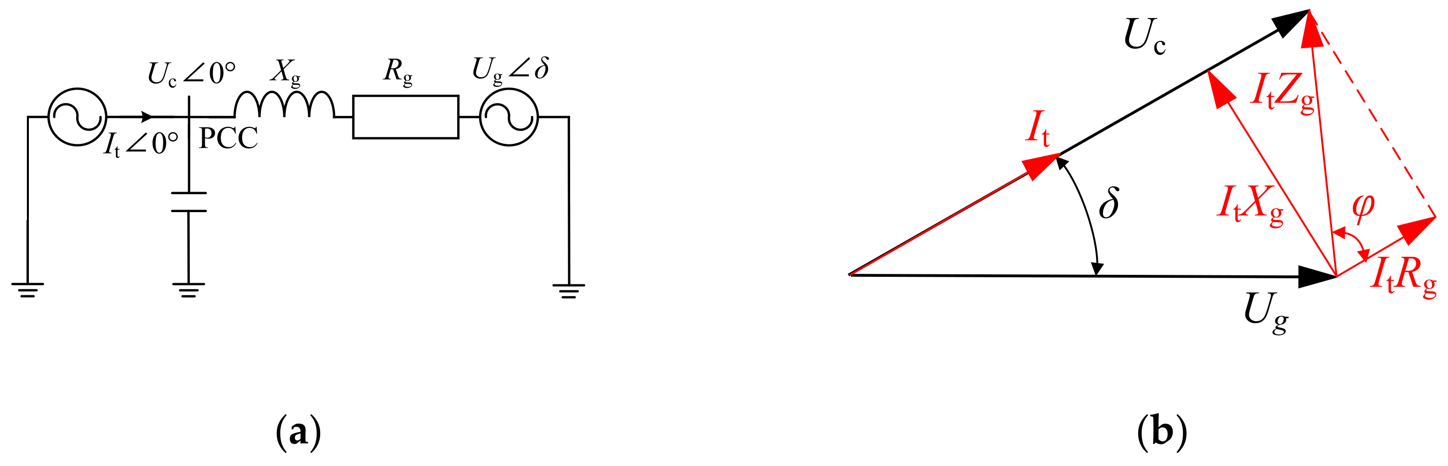
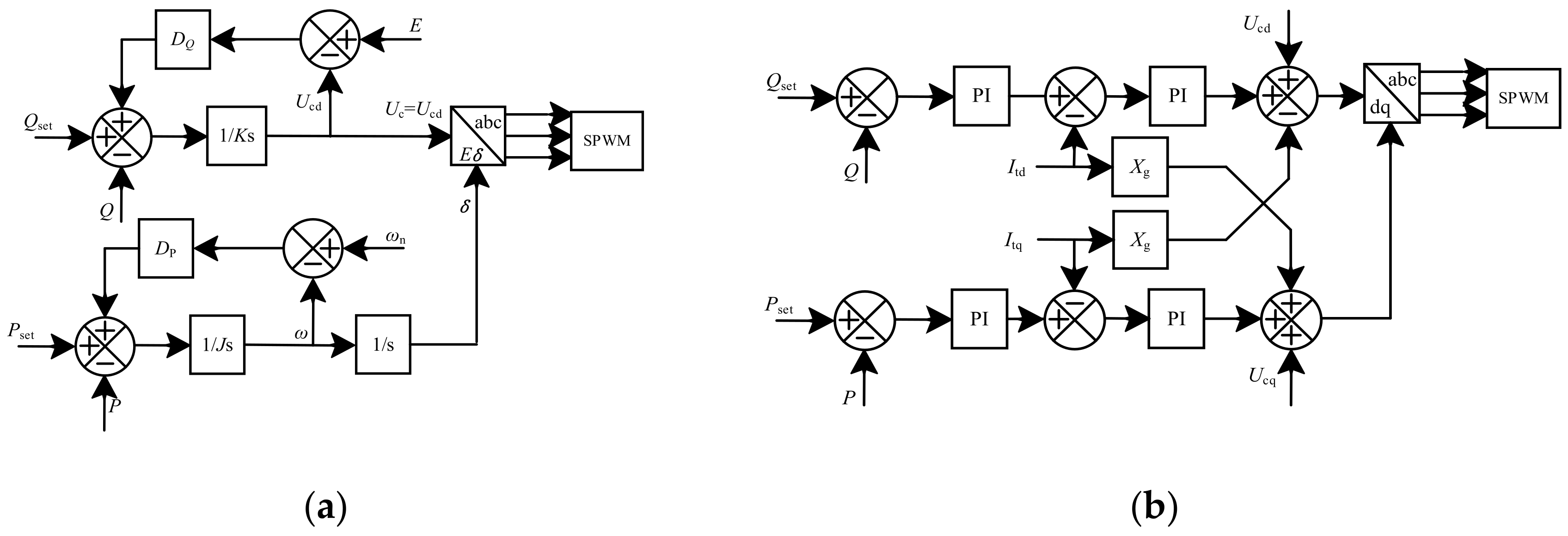
2.1. Equivalent Circuit of the GFM Converter

In Figure 1a, U_c is the RMS voltage value of the converter, and U_g is the RMS value of the grid side voltage. Assuming that the voltage at the point of common coupling (PCC) is the reference phase, the angle between the grid side voltage and the voltage at the PCC is the power-angle δ, and the line impedance R_g + jX_g = Z_g∠φ. To facilitate control and improve stability, all the reactive power is provided by reactive power compensators. The power factor of the converter is one, expressed as I_t∠0°.

The phase diagram shown in Figure 1b was drawn by combining the relationships of the variables in Figure 1a, which, in turn, gives U_c and the active power, P, transmitted by the system in three symmetrical phases:

$$U_{\mathrm{c}}=\sqrt{U_{\mathrm{g}}^2-I_{\mathrm{t}}^2{X}_{\mathrm{g}}^2}+I_{\mathrm{t}}{R}_{\mathrm{g}}$$

(1)

$$P=3U_{\mathrm{c}}{I}_{\mathrm{t}}=3\left(\sqrt{U_{\mathrm{g}}^2-I_{\mathrm{t}}^2{X}_{\mathrm{g}}^2}+I_{\mathrm{t}}{R}_{\mathrm{g}}\right)·I_{\mathrm{t}}$$

(2)

As shown in Figure 2a, the P–I_t curve can be plotted for different line impedance ratios after the transmission of active power P and current I_t has been normalized. When I_t increases, P exhibits an overall trend of increasing and then decreasing; thus, there is an extreme point which is the maximum value, P_max, referring to the maximum power that the converter can transmit in the unity power factor state. As the line impedance angle, φ, increases, the resistive component of the line impedance decreases, and the maximum power, P_max, that can be transmitted by a GFM converter will also decrease. As shown in Figure 2a, when the converter is commanded to transmit power P_set, for R_g/X_g = 1 and R_g/X_g = 0.5 grids, there is a stable static operating point, i.e., the left intersection of curves; for the R_g/X_g = 0 grid, there is no intersection, so static instability and other severe phenomena will occur.

Replacing X_g and R_g in Equation (2) with the impedance modulus Z_g and the impedance angle φ by equivalents X_g = tanφ/(1 + tan²φ)^(1/2) and R_g = (1 + tan²φ)^(−1/2), Equation (3) can be derived, and with the aid of the mathematical application Wolfram Alpha, the explicit analytical solution for P_max can be displayed as in Equation (4):

$$P=3\left(I_{\mathrm{t}}\sqrt{U_{\mathrm{g}}^2-I_{\mathrm{t}}^2{Z}_{\mathrm{g}}^2\frac{{\tan }^2\phi }{1+{\tan }^2\phi }}+\frac{Z_{\mathrm{g}}}{\sqrt{1+{\tan }^2\phi }}{I}_{\mathrm{t}}^2\right)$$

(3)

$$P_{\max }=P\left(I_{\mathrm{t}}\right)\left|{}_{I_{\mathrm{t}}=I_{\mathrm{pmax}}}\right.=\frac{3U_{\mathrm{g}}^2}{2Z_{\mathrm{g}}}·\frac{\sqrt{1+{\tan }^2\phi }}{\sqrt{1+{\tan }^2\phi }-1},\hspace{1em}{I}_{\mathrm{pmax}}\approx \frac{U_{\mathrm{g}}}{\sqrt{2}{Z}_{\mathrm{g}}}$$

(4)

From Equation (4), we can derive Figure 2b; when Z_g and φ increase, P_max will be reduced, and the specific analysis will be combined with the SCR in Section 3.1.

However, in real operation conditions, especially in weak grids, converters may be called upon to provide the necessary reactive power to support the power system and compensate the voltage drop of the original transmission line using locally installed reactive power compensators [14]; notably, the required reactive power from compensators can be considerably high which makes the installation of them costly.

As shown in Figure 3a, the phasor diagram illustrates how GFM converters provide approximately 0.7P reactive power, which is required by grids with θ which means a power factor angle of I_t. Similarly, we can derive P in the variable power factor in Equation (5).

$$\begin{array}{cc}\hfill P& =U_{\mathrm{c}}{I}_{\mathrm{tp}}=(\sqrt{U_{\mathrm{g}}^2-{(I_{\mathrm{tp}}{X}_{\mathrm{g}}-I_{\mathrm{tq}}{R}_{\mathrm{g}})}^2}+I_{\mathrm{tp}}{R}_{\mathrm{g}}+I_{\mathrm{tq}}{X}_{\mathrm{g}})I_{\mathrm{tp}}\hfill \\ & =I_{\mathrm{t}}\cos \theta \sqrt{U_{\mathrm{g}}^2-I_t^2{(X_{\mathrm{g}}\cos \theta -R_{\mathrm{g}}\sin \theta )}^2}+I_t^2(R_{\mathrm{g}}{\cos }^2\theta +\frac{X_{\mathrm{g}}}{2}\sin 2\theta )\hfill \end{array}$$

(5)

As shown in Figure 3b, for the R_g/X_g = 0 grid, P reached the highest at 0.5 (p.u.) when I was near 0.7 (p.u.). Keep the I and change the converter’s power factor, and it turns out that P reached the highest value when the θ neared 0.6 rad and was higher than 0.5 (p.u.) when the θ value was smaller than 1.0 rad. By decreasing the power factor in a large scale, GFM converters can provide an even higher active power. Therefore, although power transmission with variable power factors is very complicated, some aspects of which are beyond the scope of this study, it can be concluded that converters can meet the requirements of rated active power with or without providing sufficient reactive power; this paper focuses more on the state of unity power factor to simplify the question.

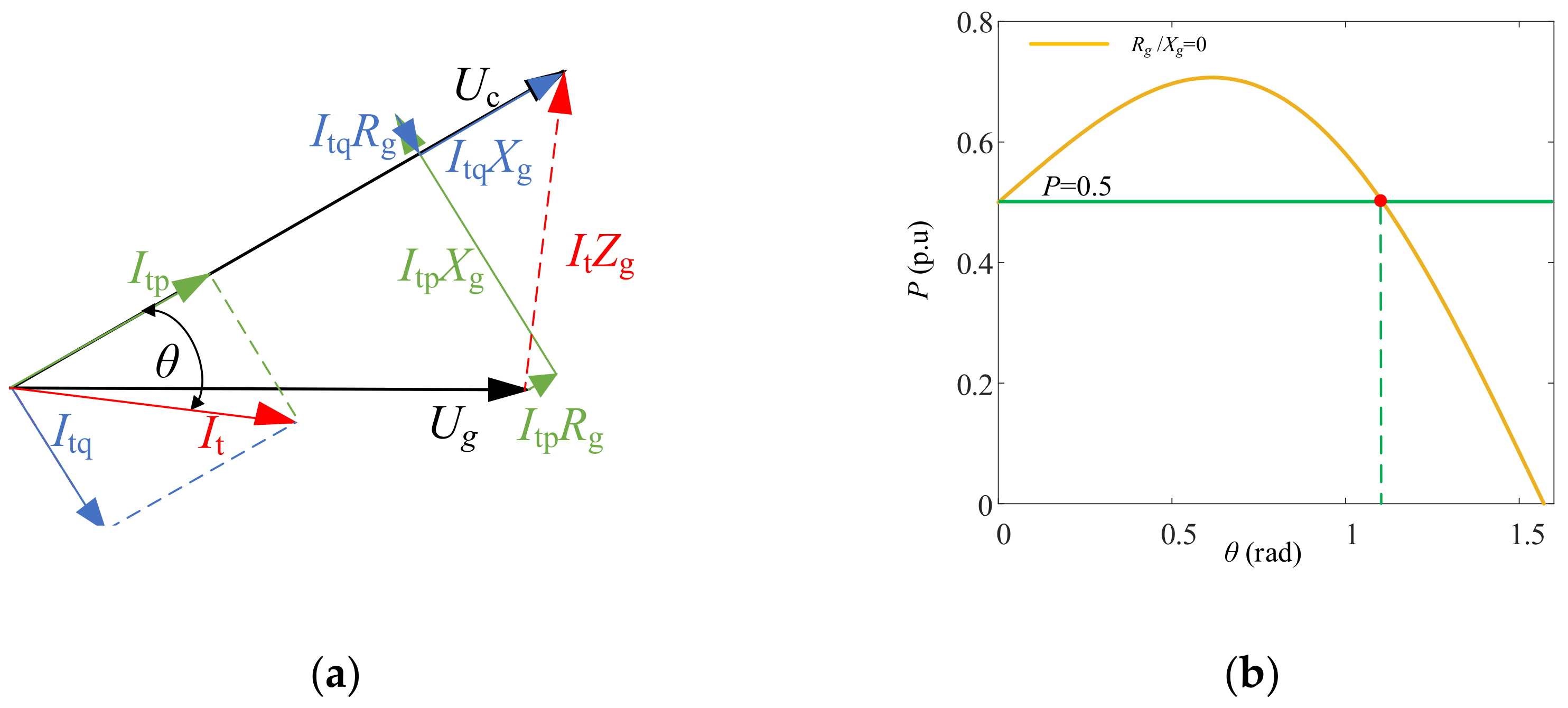
2.2. Equivalent Circuit of the GFL Converter

As shown in Figure 4a, compared with Figure 1a, due to the presence of the reactive power compensation capacitor, X_c [16], the output current is not equal to the output current, Ig, from the PCC to the grid side when the GFL converter is considered as a current source; the output voltage is still equal to the voltage at the PCC when the GFL converter is considered as a voltage source, so the model of the GFL converter is slightly more complex. The GFL converter is regarded as a current source whose output current is decoupled by dq through Park transformation and the PLL control strategy in the GFL converter [10]. The dq decoupling analysis method of currents is more suitable for GFL than GFM converters, not only because the GFL converter is a current source which should be focused more in its output current, but also due to its current inner loop control, which will be further discussed in Section 3.2. The quantitative relationship is I_gd = I_td, I_gq = U_td/X_c.

Combining the relationship and the diagram in Figure 4b, the voltage at the PCC can be derived as shown in Equation (6). Under static stability conditions, PLL accurately tracks the current; thus, U_td = U_t can be substituted into Equation (6) to obtain Equation (7). In general, the reactance to ground at the PCC X_c is much greater than the inductive reactance in the X_g grid, i.e., X_c/(X_c − X_g) = 1; thus, Equation (7) is formally identical to Equation (2). Similarly, the maximum transmission power of a GFL converter can be presented as Equation (8).

$$P_{\max }=\sqrt{U_{\mathrm{g}}^2-I_{\mathrm{gd}}^2{X}_{\mathrm{g}}^2}+I_{\mathrm{gd}}{R}_{\mathrm{g}}+I_{\mathrm{gq}}{X}_{\mathrm{g}}=\sqrt{U_{\mathrm{g}}^2-I_{\mathrm{td}}^2{X}_{\mathrm{g}}^2}+I_{\mathrm{td}}{R}_{\mathrm{g}}+\frac{U_{\mathrm{td}}}{X_{\mathrm{c}}}{X}_{\mathrm{g}}$$

(6)

$$U_{\mathrm{c}}=\frac{X_{\mathrm{c}}}{X_{\mathrm{c}}-X_{\mathrm{g}}}\left(\sqrt{U_{\mathrm{g}}^2-I_{\mathrm{td}}^2{X}_{\mathrm{g}}^2}+I_{\mathrm{td}}{R}_{\mathrm{g}}\right)$$

(7)

$$P_{\max }=\frac{X_{\mathrm{c}}}{X_{\mathrm{c}}-X_g}·\frac{3U_{\mathrm{g}}^2}{2Z_{\mathrm{g}}}·\frac{\sqrt{1+{\tan }^2\phi }}{\sqrt{1+{\tan }^2\phi }-1}$$

(8)

The form of Equation (8) is the same as Equation (4); judging from the equivalent circuit diagram, the ultimate transmission capacity in the unity power factor state is the same for both GFM and GFL converters under static stability conditions. It is a useful conclusion and means that the type of converter can be ignored when considering the ultimate transmission capacity of the converter alone.

3. Relationship between Static Power Transmission of the Converter and Grid Strength

3.1. Influence of Power Grid Strength Variation on the Steady Working Area of the System

According to the relative definition of SCR used to measure power grid strength in traditional power systems, the power grid strength of a grid-connected system with GFM and GFL converters can also be expressed by SCR [15]: the larger its value, the higher the strength of the system.

Equation (9) defines the SCR in renewable energy power grids: P_sc is the short circuit capacity of the grid, P_sc = 3$U_{\mathrm{g}}^2$/Z_g; U_g is the RMS value of the grid phase voltage; Z_g is the impedance modulus value of the grid; and P_N is the rated transmission power of the converters, which is equal to the P_set value in the GFM and GFL converters mentioned above. Thus, the strength of the power grid is not only related to the power grid itself, but also to the converter, which is jointly determined by both.

It seems that the definition of the SCR requires analyses of both converters and grids; however, because the transmission power limit of GFM converters is similar to that of GFL converters, it can reasonably be assumed that the rated transmission power of the two converters is equal, to determine the steady working area by only discussing the characteristics of the power grid itself using the SCR theory.

According to Equation (8) and Figure 2b, as Z_g increases continuously, SCR decreases, and P_max also decreases rapidly. However, when φ increases, the power grid strength increases, and P_max increases. Moreover, power grids connected to the converter are mostly of high voltage, whose φ is almost 90°; in this case, the line impedance angle has little effect on the improvement in P_max. In summary, as Z_g increases, the grid’s stiffness reduces, the SCR decreases, and P_max decreases.

Furthermore, the steady working area requires P_set ≤ P_N; according to Equations (8) and (9), the constraint relationship between the transferable power (steady working area) of converters and power grid strengths under static stability can be calculated as Equation (10).

Notably, although the minimum SCR increases with the increase in impedance angle, it always exists at SCR_min ≤ 2, which is consistent with the conclusion that the SCR of a very weak power grid is less than 2, and further verifies the accuracy of the conclusion.

$$\mathrm{SCR}=\frac{P_{\mathrm{sc}}}{P_{\mathrm{N}}}=\frac{3U_{\mathrm{g}}^2}{Z_{\mathrm{g}}·P_{\mathrm{set}}}$$

(9)

$$\left\{\begin{array}{l}{P}_{\mathrm{set}}\le \frac{3U_{\mathrm{g}}^2}{2Z_{\mathrm{g}}}·\frac{\sqrt{1+{\tan }^2\phi }+{\tan }^2\phi +1}{{\tan }^2\phi }\\ \mathrm{SCR}\ge 2-\frac{2(\sqrt{1+{\tan }^2\phi }+1)}{\sqrt{1+{\tan }^2\phi }+{\tan }^2\phi +1}\end{array}\right.$$

(10)

3.2. Influence of Power Grid Strength on the Power Transmission of Converters

As shown in Figure 5a, the block diagram of a GFM converter was used to further analyze the influencing factors of its stability during transmission power, which is not only conducive to exploring whether the converter is stable when it reaches P_max, but also when exploring the stability characteristics of the converter when it transmits arbitrary power under a certain strength grid. GFM converters regulate the active and reactive power output, P and Q, to the system by controlling the output voltage, U_c, and power-angle, δ, having P = 3U_cU_gsinδ/X_g and Q = 3U_c(U_c − U_gcosδ)/X_g.

Thus, by taking the partial derivative with respect to P and Q, with ∂P/∂U_c = 3U_gsinδ/X_g, ∂Q/∂δ = 3U_cU_gsinδ/X_g, U_c and δ are expected to be taken as control quantities, P and Q are taken as controlled quantities, and the control GFM converter is a two independent single-input single-output system; thus, power coupling is not conducive to GFM converter control, which demonstrably does not meet the objective of the independent control of P and Q.

When the power grid strength decreases, SCR decreases, X_g increases, and ∂P/∂U_c decreases; therefore, the coupling relationship between P and Q decreases, and the stability of the GFM converter when transmitting P_max is further guaranteed. Notably, when P changes, the coupling relationship between P and Q does not change. Therefore, the characteristics of a GFM converter are applicable to weak grids in the steady working area of the system.

At the same time, because GFM converters continue the traditional control strategy of virtual synchronous generators (VSGs) and introduce gains, such as D_P and D_Q, when they are set to a certain value, the damping and standby inertia of the system is sufficient, and the power transmission is smoothly regulated within the limit range because the impedance of the weak grid is large. However, when the grid strength increases, the impedance decreases. Due to the limitation of VSG parameters, high-frequency oscillations may occur during power transmission due to parameter mismatch, which is not conducive to system stability. This further verifies that GFM converters are not suitable for strong grids.

As shown in Figure 5b, GFL converters regulate P and Q by controlling the d- and q-axis components of the output current, I_td and I_tq, respectively. As shown in Figure 4b, the converter is in a state of unity power factor; thus, I_t = I_td, and its P–I_td curve is similar to the curve in Figure 2a. When I_td increases, the operation is stable if P increases monotonically, and may be statically unstable if the monotonicity of P changes. The P–I_td curve is a convex function; therefore, it is concluded that the ultimate transmission power of GFL converters is the same as P_max in Equation (4), and as such, GFL converters are more suitable for higher-strength grids. Additionally, when the grid strength is high, due to the small impedance of the system, the time constant requirement is not high, and the power can be smoothly adjusted within the specified time; when the grid strength decreases, due to the rising impedance of the system, the power may not be adjusted within the specified time. If PI parameters are not set reasonably and the converter itself is adjusted too fast, it will produce an overshoot and a shock on the grid, which further verifies that GFL converters are more suitable for strong grids.

4. Simulation Waveform Analysis

Simulated waveforms are used to further verify the characteristics of GFM and GFL converters in transmitting power at different grid strengths. Assuming that the systems connected to the converter are all high-voltage grids, the grid strength is changed by varying the inductive reactance parameters in the line. More details about the simulation in PLECS are shown in

Table 1. Parameters of systems of three grid strengths.

Phase Voltage Ug (V)	Rg (Ω)	Xg (Ω)	SCR	Pmax (W)
220	0.1	0.50	29.04	145,200
		3.00 10.00	4.84	25,000
			1.45	7300

,

Table 2. Parameters of systems of the GFM converter.

J/(kg·m2)	Dp	Dq	K
0.057	5	321	7.1

and

Table 3. Parameters of systems of the GFL converter.

Kp_PLL	Ki_PLL	Kp_i	Ki_i
0.7978	99.0138	0.0043	0.7143

.

As shown in Table 1, it is assumed that the rated transmission power of both GFM and GFL converters is constant, and since the SCR is generally considered to be stronger than 20 for a strong grid and less than 2 for a very weak grid, it was reasonable to set the SCR to 29.04, 4.84, and 1.45 for this simulation.

Table 2 and Table 3 show the parameters of GFM and GFL converter systems; the simulation was performed to verify the transmission capacity rather than modify converters, so these parameters were kept the same during the simulation.

4.1. Simulation of GFM Converter Power Transfer When SCR = 4.84

The main purpose of the grid-connected simulation model with an SCR of 4.84 is to reduce the influence of the grid strength on both converters, and thus, to observe the influence of the systems own power transmission limit on the converters’ transmission power. As shown in Figure 6a, the actual value of P_max is slightly lower than the theoretical value (25,000 W) due to the limitations of GFM converter parameter adjustments. When the commanded power transmission is 22,000 W, the converter can deliver a rapid response within 1 s and reach the static stable equilibrium, as expected.

As shown in Figure 7, the GFM converter has high output current sinusoidality, low harmonics, and high immunity to interference at a statically stable transmission of 22,000 W, further verifying its good static stability performance. When the converter command rose from 22,000 W to 25,000 W, the actual power transmitted by the converter will rise steadily to 25,000 W; however, at this time, the converter cannot work in the unity power factor state, so it will output a certain amount of reactive power steadily to the outside. At this time, the converter output current is stable, as shown in Figure 7.

When the active power command continues to increase, the converter cannot transmit the active power evenly when compensated by infinite reactive power. However, as shown in Figure 8a, when the active power command increases from 25,000 W to 50,000 W, the converter can only transmit about 40,000 W with high reactive power, so the system will be in a state of static instability and the output active power will be in a state of low-frequency oscillation (at a frequency of approximately 1 Hz). The reason is that the change in power-angle, δ, at this time cannot meet the requirements of active power instruction, so the power angle oscillates at low frequency, and the reactive power oscillates synchronously with the active power. In this case, although the converter’s output current oscillates, it has a good sinusoidal degree and no obvious harmonics, as shown in Figure 8b.

4.2. Simulation of GFL Converter Power Transfer When SCR = 4.84

Similarly, when a GFL converter is commanded to transmit at 22,000 W, it still responds quickly and has little harmonics. When P_set is raised to 25,000 W, P slowly rises to slightly above the command, then becomes out of control and quickly rises to another stable operating point; the value of P is determined by the converter itself as long as P_set exceeds the limit power. The reason is shown in Figure 9b, as Q first operates out of control and cannot be stabilized in a smaller range, resulting in a sharp increase in Q, which further leads to a runaway P value, but at this point, Q can be as high as 40,000 var and a certain degree of harmonics is injected into the grid, as shown in Figure 10. The fifth and seventh harmonics indicate that Q is so high that it exceeds the GFL converter’s transmission limit and causes instability. Due to the power coupling of a GFM converter, the reactive power does not become out of control; only a stable offset occurs, as shown in Figure 6.

4.3. Comparison of the Power Transfer Capability of Converters at Strong and Weak Grid Strengths

A simulation model for a strong grid with a SCR greater than 20 and a weak grid with SCR less than 2 was established to compare the influence of the grid strength on the transmission of power within the limit range of GFM and GFL converters.

As shown in Figure 11, when the P_set of the very weak grid was 7300 W, it could reach the target requirement within 1–2 s, whereas I_t and U_c have little harmonic similarity to that depicted in Figure 7: when the P_set of the strong grid reached 140,000 W (slightly below the ideal limit), it could respond rapidly in about 0.1 s, whereas U_c had high fifth and seventh harmonics, as shown in Figure 12, which is due to the large influence of power coupling to make the control quantity U_cd exceed normal levels and the PWM of the GFM converter to become far from sinusoidal. High harmonics from both GFM and GFL converters are caused by the runaway of control quantities, although specific reasons are different. GFM converters set a fixed virtual impedance in the face of a strong grid with a small impedance, which does not match the grid, resulting in a high frequency oscillation of U_c with a frequency of approximately 100 Hz; in contrast, the weaker grid impedance is larger, which offsets the virtual impedance setting problem and smooths the power output of the converter.

As shown in Figure 13, GFL converters can output P_max relatively more rapidly under both weak and strong grid conditions, with I_t and U_c having small harmonics. The PI controller time constant here is fixed at approximately 0.5 s; when the GFL converter runs on the weak grid, its regulation speed is higher than the grid, so P has obvious oscillation overshoot. At the same time, there is no virtual impedance setting in the GFL converter, so the regulation time is not too fast but relatively smooth in strong grids.

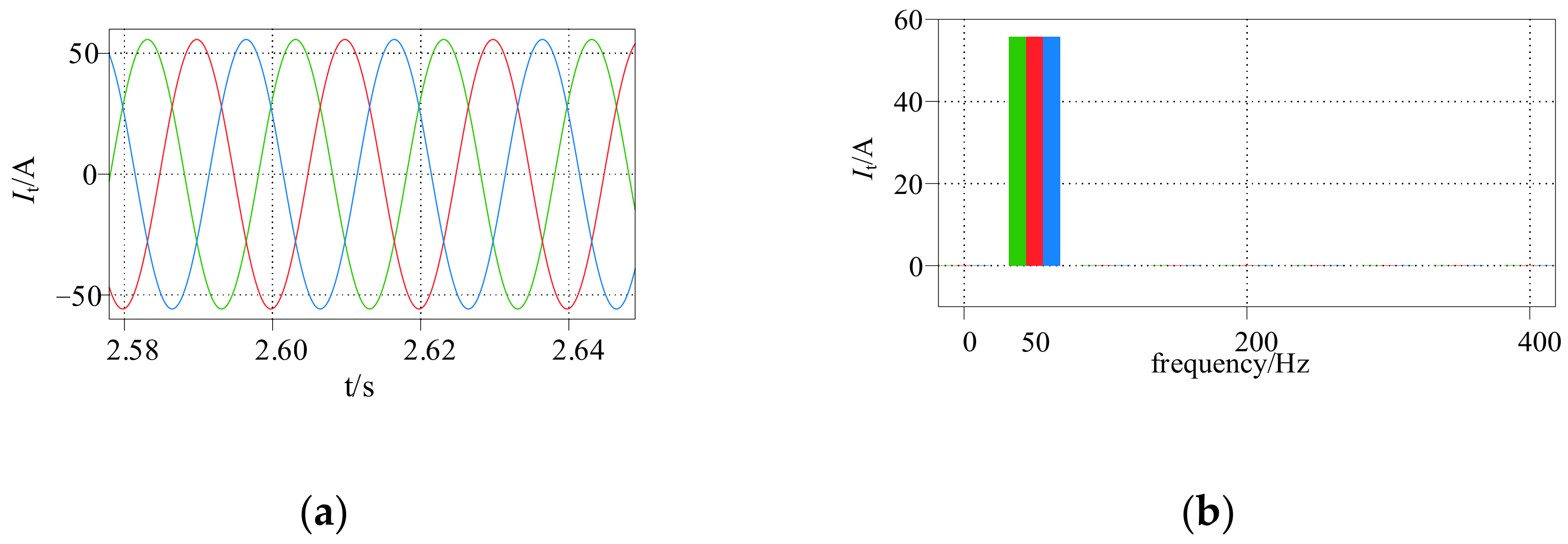
4.4. Hardware in-Loop Simulation Using RTBOX1

Figure 14 shows the real-time simulation devices RTBOX1 and F28379D launchpad. Using this platform facilitates the verification of the above conclusions. Figure 15 shows two states of transmitting power by GFM or GFL converters; the simulation waveform characteristics, such as harmonics, are similar to those in PLECS, which further verifies that their transmission capacity could be realized in actual power grids.

5. Conclusions

This study investigated the transfer capabilities of the two main types of non-synchronous machine power sources connected to GFM and GFL grids, focusing on the transfer capability of converters at different grid strengths based on their static and stable operation.

• There is a quantitative relationship between the statically stable power transmission limit and the line impedance of GFM and GFL converters at a unity power factor. At variable power factors, the converters can even transmit active rated power sufficiently. For high-voltage grids, the reactance, X_g, increases; its impedance modulus, Z_g, increases. SCR decreases, P_max decreases, and the operating range is reduced. However, when X_g increases, its impedance angle, φ, increases, and P_max increases, but the impact of φ on the transmission capacity is much smaller than that of Z_g. Therefore, the larger the impedance, the smaller the P_max; thus, the two are approximately inversely related.
• The grid strength of a system is determined by SCR, which is jointly influenced by Z_g and the rated transmission power of the converter. When the reactance of PCC to ground is much greater than X_g, the P_max values of GFM and GFL converters are equal, and it can be considered that the grid strength is only related to X_g, i.e., the greater the grid strength, the greater the P_max.
• Within P_max (in a steady working area), GFM converters are more suitable for weak grids because of the power coupling problem, which is more obvious in strong grids, whereas GFL converters are more suitable for strong grids because of the monotonic nature of the current in the P–I_t curve. Moreover, in smoothing power transfer, the parameters of GFM converters, which require virtual impedance settings, make them more suitable for weak grid regulation because they are prone to high-frequency oscillations under strong grids. GFL converters, however, with their parameters of time constants and PI controllers, are more suitable for the regulation of strong grids because they are prone to overshooting oscillations in weak grids.

References

1. Huang, C.; Zheng, Z.; Ma, X.; Yan, H.; Wang, M.; Fan, Z. Research on the influence of resilient grid learning ability on power system. Energy Rep. 2022, 8, 43–50. [Google Scholar] [CrossRef]
2. Granata, S.; Di Benedetto, M.; Terlizzi, C.; Leuzzi, R.; Bifaretti, S.; Zanchetta, P. Power Electronics Converters for the Internet of Energy: A Review. Energies 2022, 15, 2604. [Google Scholar] [CrossRef]
3. Amin, M.; Molinas, M. Small-signal stability assessment of power electronics based power systems: A discussion of impedance-and eigenvalue-based methods. IEEE Trans. Ind. Appl. 2017, 53, 5014–5030. [Google Scholar] [CrossRef]
4. Iioka, D.; Kusano, K.; Matsuura, T.; Hamada, H.; Miyazaki, T. Appropriate Volt–Var Curve Settings for PV Inverters Based on Distribution Network Characteristics Using Match Rate of Operating Point. Energies 2022, 15, 1375. [Google Scholar] [CrossRef]
5. Khan, S.A.; Wang, M.; Su, W.; Liu, G.; Chaturvedi, S. Grid-Forming Converters for Stability Issues in Future Power Grids. Energies 2022, 15, 4937. [Google Scholar] [CrossRef]
6. Yap, K.Y.; Sarimuthu, C.R.; Lim, J.M.-Y. Virtual Inertia-Based Inverters for Mitigating Frequency Instability in Grid-Connected Renewable Energy System: A Review. Appl. Sci. 2019, 9, 5300. [Google Scholar] [CrossRef] [Green Version]
7. Vadi, S.; Padmanaban, S.; Bayindir, R.; Blaabjerg, F.; Mihet-Popa, L. A Review on Optimization and Control Methods Used to Provide Transient Stability in Microgrids. Energies 2019, 12, 3582. [Google Scholar] [CrossRef] [Green Version]
8. Zhang, S.; Zhu, Z.; Li, Y. A Critical Review of Data-Driven Transient Stability Assessment of Power Systems: Principles, Prospects and Challenges. Energies 2021, 14, 7238. [Google Scholar] [CrossRef]
9. Hosseinzadeh, N.; Aziz, A.; Mahmud, A.; Gargoom, A.; Rabbani, M. Voltage Stability of Power Systems with Renewable-Energy Inverter-Based Generators: A Review. Electronics 2021, 10, 115. [Google Scholar] [CrossRef]
10. Pattabiraman, D.; Lasseter, R.H.; Jahns, T.M. Comparison of grid following and grid forming control for a high inverter penetration power system. In Proceedings of the 2018 IEEE Power & Energy Society General Meeting (PESGM), Portland, OR, USA, 5–10 August 2018; pp. 1–5. [Google Scholar]
11. Poolla, B.K.; Groß, D.; Dörfler, F. Placement and implementation of grid-forming and grid-following virtual inertia and fast frequency response. IEEE Trans. Power Syst. 2019, 34, 3035–3046. [Google Scholar] [CrossRef] [Green Version]
12. Awal, M.A.; Husain, I. Unified virtual oscillator control for grid-forming and grid-following converters. IEEE J. Emerg. Sel. Top. Power Electron. 2020, 9, 4573–4586. [Google Scholar] [CrossRef]
13. Chen, X.; Zhang, Y.; Wang, S.; Chen, J.; Gong, C. Impedance-phased dynamic control method for grid-connected inverters in a weak grid. IEEE Trans. Power Electron. 2016, 32, 274–283. [Google Scholar] [CrossRef]
14. Yang, D.; Wang, X.; Liu, F.; Xin, K.; Liu, Y.; Blaabjerg, F. Adaptive reactive power control of PV power plants for improved power transfer capability under ultra-weak grid conditions. IEEE Trans. Smart Grid 2017, 10, 1269–1279. [Google Scholar] [CrossRef] [Green Version]
15. Kang, Y.; Lin, X.; Zheng, Y.; Quan, X.L.; Hu, J.B.; Yuan, S. The static stable-limit and static stable-working zone for single-machine infinite-bus system of renewable-energy grid-connected converter. Proc. CSEE 2020, 40, 4506–4515. [Google Scholar]
16. Chen, M.; Zhou, D.; Tayyebi, A.; Prieto-Araujo, E.; Dörfler, F.; Blaabjerg, F. Generalized multivariable grid-forming control design for power converters. IEEE Trans. Smart Grid 2022, 13, 2873–2885. [Google Scholar] [CrossRef]
Figure 1. (a) Equivalent circuit diagram of the GFM converter; (b) phasor diagram of the GFM converter with unity power factor.
Energies 16 02594 g001
Figure 2. (a) PIt curves for different line impedance ratios; (b) plot of Pmax and Zg, φ.
Energies 16 02594 g002
Figure 3. (a) Phasor diagram of the GFM converter provides the required reactive power; (b) plot of P and θ.
Energies 16 02594 g003
Figure 4. (a) Equivalent circuit diagram of a GFL converter; (b) phasor diagram of GFL converter.
Energies 16 02594 g004
Figure 5. (a) Block diagram of a GFM converter; (b) block diagram of a GFL converter.
Energies 16 02594 g005
Figure 6. (a) Active power of a GFM converter (Pset = 22,000 W, SCR = 4.84); (b) reactive power of a GFM converter (Pset = 25,000 W, SCR = 4.84).
Energies 16 02594 g006
Figure 7. (a) Current curve of a GFM converter (Pset = 25,000 W, SCR = 4.84); (b) current THD of a GFM converter (Pset = 25,000 W, SCR = 4.84). (Green for phase A, red for phase B, blue for phase C).
Energies 16 02594 g007
Figure 8. (a) Active power of a GFM converter (Pset = 50,000 W, SCR = 4.84); (b) current of a GFM converter (Pset = 50,000 W, SCR = 4.84).
Energies 16 02594 g008
Figure 9. (a) Active power of a GFL converter (Pset = 25,000 W, SCR = 4.84); (b) reactive power of a GFL converter (Pset = 25,000 W, SCR = 4.84).
Energies 16 02594 g009
Figure 10. (a) Current of a GFL converter (Pset = 25,000 W, SCR = 4.84); (b) current THD of a GFL converter (Pset = 25,000 W, SCR = 4.84). (Green for phase A, red for phase B, blue for phase C).
Energies 16 02594 g010
Figure 11. (a) Active power of a GFM converter (Pset = 7000 W, SCR = 1.45); (b) active power of a GFM converter (Pset = 140,000 W, SCR = 29.04).
Energies 16 02594 g011
Figure 12. (a) Voltage of a GFM converter (Pset = 140,000 W, SCR = 29.04); (b) THD of a GFM converter (Pset = 140,000 W, SCR = 29.04). (Green for phase A, red for phase B, blue for phase C).
Energies 16 02594 g012
Figure 13. (a) Active power of the GFL converter (Pset = 7000 W, SCR = 4.84); (b) active power of the GFL converter (Pset = 140,000 W, SCR = 4.84).
Energies 16 02594 g013
Figure 14. RTBOX1 and F28379D launchpad.
Energies 16 02594 g014
Figure 15. (a) Voltage of the GFM converter (Pset = 140,000 W, SCR = 29.04); (b) current of the GFL converter (Pset = 22,000 W, SCR = 4.84). (Green for phase A, red for phase B, blue for phase C).
Energies 16 02594 g015