1. Introduction
Human society is currently facing, and will continue to face, serious problems such as resource shortages and global climate change. Avoiding this dilemma requires two changes to the world’s energy mix: a clean energy alternative on the power supply side and an electric energy alternative on the energy consumption side. This work is about electricity consumption. According to local and global statistics, energy consumption follows a rising trend, with electricity accounting for nearly 21% of total energy consumption in 2021 [
1].
As the world becomes more dependent on electricity, planning for power generation is critical. Additionally, electric energy may be stored, while electricity may not. On the other hand, electricity is typically utilized shortly after it is generated. This increases the need for energy suppliers to plan their power delivery. Central planning specifications are reliable predictions of future power consumption. In particular, medium- to long-term forecast accuracy of electricity consumption is vital for energy system programming and planning. However, inaccurate prediction of power consumption can be a disadvantage. Overestimation will lead to the wastage of valuable energy resources, large capital expenditures, and long construction periods. Underestimation has far-reaching negative consequences, such as blackouts. Of course, if beneficial early warnings based on high power consumption prediction accuracy are provided, some precautions can be taken to avoid adverse consequences. Additionally, the time series of electricity consumption is uncertain, complex, and nonlinear, dependent on the political situation, economics, human activities, population behavior, climatic factors, and other external factors that affect the accuracy of electricity consumption forecasts [
2,
3,
4,
5,
6].
It is well known that electricity consumption/demand time series display distinct characteristics. The monthly consumption time series may exhibit an annual cyclic pattern and a linear or nonlinear long-term trend. Weather and societal variables have a significant impact on electricity usage, which is shown in the consumption time series. Additionally, economic variables frequently impact the trajectory of the consumption time series, while climatic variations inject a periodic behavior into the series [
7]. For instance,
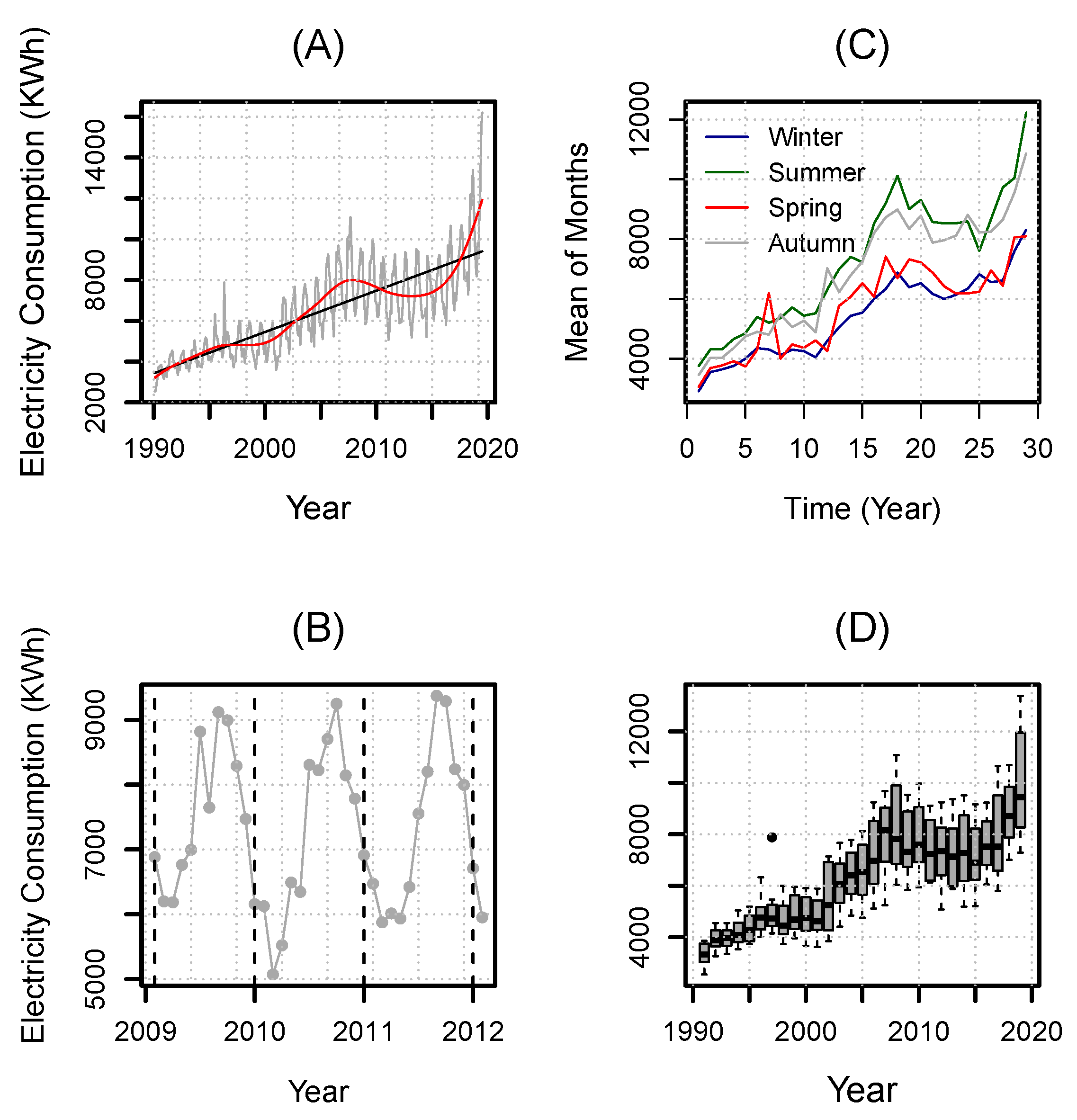
Figure 1A displays Pakistan’s electricity consumption time series for the period from January 1990 to June 2020 with superimposed linear (black line) and nonlinear (red curve) trends. The plots in
Figure 1 depict a rising nonlinear trend (
Figure 1A), different seasonal effects (
Figure 1B), a yearly periodicity (
Figure 1C), and the variation of electricity consumption in different years (
Figure 1D).
In the electricity consumption literature, many techniques have been used to forecast electric power consumption over the last thirty years. Generally, these forecasting methods can be grouped into three categories: statistical methods, models of artificial intelligence, and hybrid system approaches [
8]. Examples of statistical models include ARIMA-based models, exponential smoothing models [
9], and parametric and nonparametric regression methods. Compared with artificial neural network models, these methods are simple mathematical structures and are easy to implement. In addition, these models are widely used for power consumption forecasting [
10,
11,
12,
13,
14]. For example, Ref. [
15] provides a component-based estimation method to forecast electricity consumption in Pakistan one month in advance using various regression models and time series. To do this, the electricity consumption data are divided into two main components: deterministic and stochastic. To estimate the deterministic component, the authors use parametric and nonparametric regression models. The stochastic part is modeled using four different univariate time series models. Pakistan’s electric consumption data from January 1990 to December 2015 were used to evaluate the performance of the proposed method. Their results showed that parametric and nonparametric regression models have the highest accuracy with the combined ARMA model. Another study, Ref. [
16], predicts the hourly power consumption for Belgium and German industrial firms by applying Markov’s switching model with time-varying transition probabilities. The model consists of a heterogeneous Markov chain and an autoregressive moving average (ARMA) process with a seasonal pattern. The authors use the continuous ranking probability score (CRPS) to estimate the goodness of fit and compare probabilistic models using benchmark models from four different companies. The results show that the proposed model outperforms the traditional additive time series approach and that the Markov switching model performs well. In contrast, artificial intelligence models are more commonly used to address nonlinear load forecasting problems compared with linear time series approaches [
17,
18,
19,
20,
21]. For example, Ref. [
22] proposed a pooling-based Deep Recurrent Neural Network (PDRNN) method for forecasting household demand to address the problem of overfitting. The authors used a dataset from the smart metering electricity customer behavior trials (CBT) conducted in Ireland from 1 July 2009, to 31 December 2010. They validate the performance of the proposed method using a support vector machine (SVR), autoregressive integrated moving average (ARIMA), and three-layer deep Recurrent Neural Networks (RNN). The performance of the model was evaluated using the Root Mean Square Error (RMSE) criterion, and the results showed that the proposed model is 19.5%, 13.1%, and 6.5% more efficient than ARIMA concerning RMSE, SVR, and RNN. On the other hand, Ref. [
23] proposed an SVM model for medium-term load forecasting using the EUNITE load competition dataset. The results show that the proposed model is useful for medium-term electric demand forecasting. In another study, two-level short-term load forecasting (STLF) using Q-Learning-based dynamic model selection (QMS), developed by [
24] using the electricity demand dataset, found that the proposed technique produced the best results. Aiming at improving forecast electric power consumption, various researchers have combined the features of two or more models to build new models, commonly known as hybrid models [
25,
26,
27,
28,
29,
30,
31]. For example, Ref. [
32] proposed a hybrid model that combines features of machine learning tools (kernels) and vector regression models. The results show that the proposed hybrid model is useful for power demand forecasting. In [
33], the authors proposed an ensemble hybrid forecasting model, the ARIMA-ANFIS model, whereby they combined an ARIMA model with an adaptive neurofuzzy inference system (ANFIS). They extended the ARIMA-ANFIS model to three different patterns and applied a hybrid ensemble model to the Iranian dataset to predict energy consumption. The ARIMA model was used for the linear part, and ANFIS for the nonlinear. All the patterns were compared using different methods to check model accuracy. Their results show that the proposed methodology is more efficient and highly accurate. On the other hand, Ref. [
34] proposed an ensemble model combining a deep learning belief network (DBN) and a support vector regression (SVR) model for power load forecasting. On another topic, some authors study the effects of different environmental and globalization trends [
35,
36]. For instance, Ref. [
36] used panel estimation methods to study the impact of environmental technologies on energy demand and energy efficiency. The results of the research show that energy consumption decreases as environmental technology improves. In addition, environmental technology plays a vital role in reducing energy intensity and improving energy efficiency. However, generally, each model has its own functional and structural form, and predictive performance varies from market to market [
37,
38,
39,
40].
In contrast to the methods introduced above, another methodology that can improve performance is to preprocess the dataset to provide a more easily predicted, modified version of the time series [
41,
42]. An ordinary option when forecasting energy-related time series is to decompose the original dataset into multiple subseries that can be separately predicted and summed to provide a real-time time series forecast. The goal is to obtain a new time series that has a more or less periodic behavior and is, therefore, easy to forecast. This assumption is based on the fact that energy-related quantities are closely related and influenced by climatic and social factors that show a specific periodic behavior. Therefore, this paper proposes a new decomposition and combination methodology that is simple and easy to implement. First, the proposed decomposition methods are Regression Spline Decomposition, Smoothed Spline Decomposition, and Hybrid Decomposition. Second, the three standard time series models considered are linear autoregressive, nonlinear autoregressive, and autoregressive moving averages, to estimate each new subseries. The proposed methodology was used to obtain a one-month-ahead out-of-sample forecast of Pakistan’s monthly electricity consumption data. The individual results for the forecasting models are summed, and the final, one-month-ahead electricity consumption forecast is obtained.
The rest of the paper is designed as follows:
Section 2 describes the general procedure of the proposed forecasting methodology.
Section 3 provides an empirical application of the proposed modeling framework using the Pakistan monthly electricity consumption data.
Section 4 comprises a discussion about the proposed methodologies and some of the best models available in the literature. Finally,
Section 5 addresses the concluding remarks and future research directions.
2. The Proposed Forecasting Methodology
This section explains the proposed forecasting methodology for one-month-ahead electricity consumption forecasting. As described in the previous section, the time series of electricity consumption contain specific characteristics, such as linear or nonlinear long-run trends, monthly periodicity, and nonconstant mean and variance. Incorporating these unique characteristics into the model significantly increases forecast accuracy. To do this, the electricity consumption time series is decomposed into three new subseries: the long-term trend series, seasonal series, and stochastic series, using the proposed decomposition methods described in the following subsection.
2.1. The Proposed Decomposition Techniques
This subsection describes the general procedure for decomposing a monthly time series of electricity usage. For this purpose, the consumption time series (
) is split into three new subseries: long-term trend
, seasonal
, and stochastic
series. The mathematical representation of the decomposed subsequence is given by
Hence, for modeling purposes, the long-term trend is a function of time n, the seasonal cycle is the function of the series , and the stochastic subseries, which describes the short-run dependence of consumption series, is obtained by . Therefore, the proposed decomposition methods, including DRS (decomposition based on regression splines), DSS (decomposition based on smoothing splines), and DH (hybrid decomposition), are discussed in the following subsections.
2.1.1. Regression Spline Decomposition Method
A regression spline is a general nonparametric approximation of
by a piecewise qth degree polynomial, estimating a subinterval bounded by a series of m points (called knots). Any spline function
of order q can be defined as a linear combination of functions
called basis functions, whose formula is given by increase.
The unknown parameter is , estimated by the ordinary least squares method. The most important choices are the number of nodes and their positions, which define the smoothness of the approximation. In this work, we used cross-validation to estimate these quantities.
2.1.2. Smoothing Splines Decomposition Method
To meet the requirements for resolving knot regions, spline features can be predicted using a least-squares penalty environment to limit the sum of squares. Hence, the equation can be written as
where
is the second derivative of
. The first term describes the goodness of fit, and the second term penalizes the coarseness of the function by the smoothing parameter
. Moreover, the selection of smoothing parameters is a difficult task and is performed using cross-validation methods in this work.
In the hybrid decomposition method, we decomposed the long-term series () with a regression spline and the seasonal series with a smoothing spline.
2.1.3. Seasonal Trend Decomposition Method
To assess the performance of the three proposed decomposition methods, they are compared with a standard and benchmark decomposition method, the Seasonal Trend Decomposition (DSTL). Cleveland et al. [
43] proposed a decomposition method where a seasonal time series is divided into trend, seasonal and stochastic components. DSTL uses LOESS to divide the seasonal time series into trend, seasonal, and stochastic components. In particular, the steps for DSTL are: (i) detrending; (ii) periodic smoothing of subsequences: creating a sequence for each seasonal component and smoothing them separately; (iii) low-pass filtering smoothing of regular substrings: recombining and smoothing substrings; (iv) season series cleanup; (v) detrending the original series using the seasonal component calculated in the previous step; and (vi) smoothing the seasonal sequence to obtain the trend component.
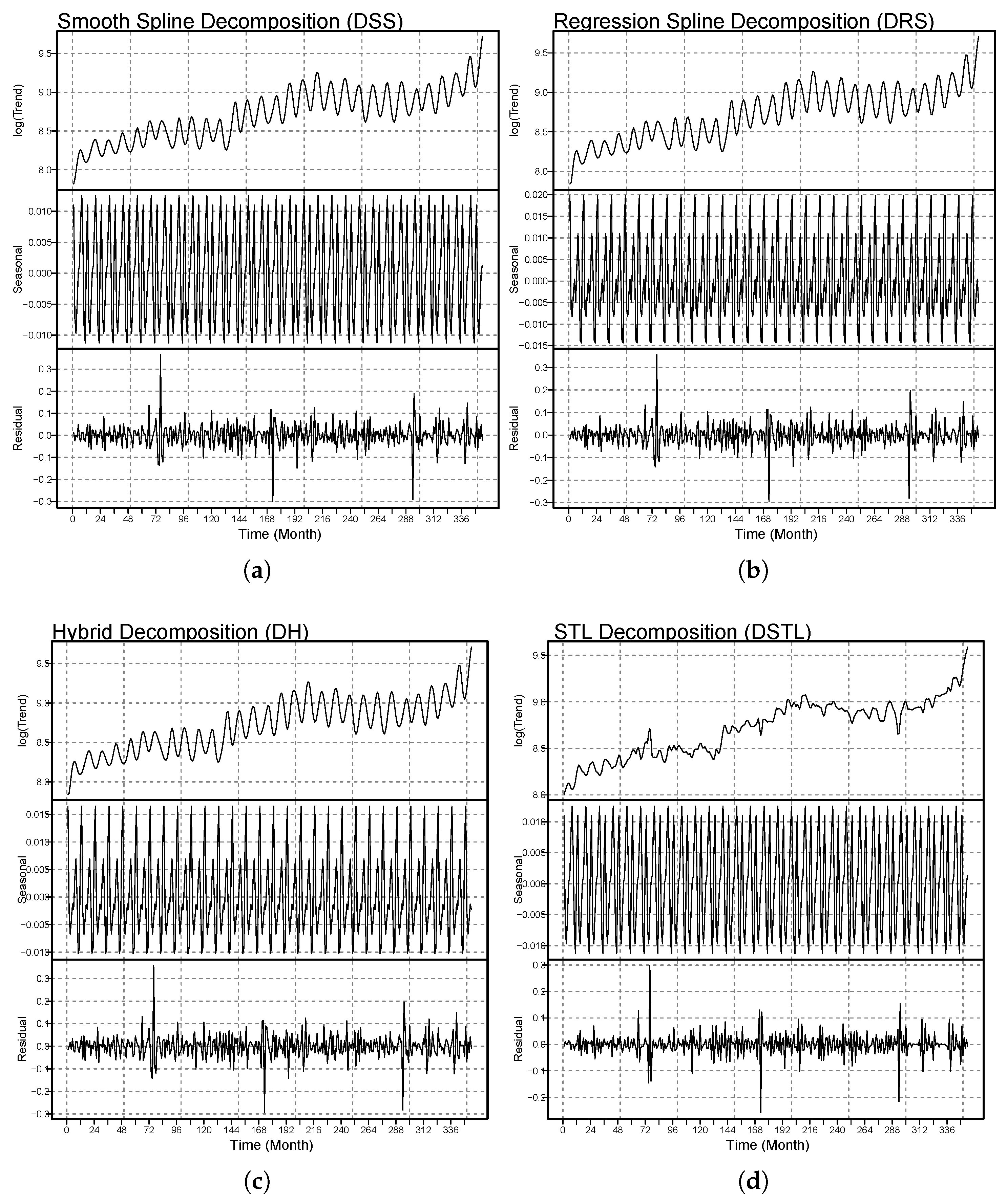
To graphically demonstrate and compare the performance of the three proposed decomposition methods described above and the benchmark DSTL decomposition, the decomposed subseries are shown in
Figure 2. In each of the
Figure 2a–d, the top panel shows the long-term trend (
), the middle panel shows the seasonal component (
), and the bottom panel shows the stochastic component (
). All of the proposed decomposition methods and the benchmark decomposition method were used to decompose (
) to adequately capture the long-term nonlinear trend and monthly periodicity of the power consumption series. Moreover, the proposed decomposition methods accurately compared the extracted features with the benchmark method. In particular, of the proposed decomposition methods, the DH method has extracted the dynamic very well compared with the other methods.
2.2. Modeling the Decomposed Subseries
Once the subseries are extracted from the monthly electricity consumption time series using the above proposed decomposition methods and benchmark decomposition method, the extracted subseries are fitted using the three considered standard time series models (linear autoregressive, nonlinear autoregressive, and autoregressive moving averages). These three models are explained in the following subsections.
2.2.1. Linear Autoregressive Model
A linear autoregressive (LAR) model uses a linear combination of
p past observations of
to describe the short-term dynamics of
, and can be written as
where
are the AR parameters and
is the white noise process. In the current study, parameters are estimated using maximum likelihood estimation. After plotting the Autocorrelation Function (ACF) and Partial Autocorrelation Function (PACF) of the series, we concluded that lags 1, 2, and 12 were significant and therefore included them in the model.
2.2.2. Nonlinear Autoregressive Model
The nonlinear additive counterpart of LAR is the nonlinear additive model (NLAR), where the relationship between
and its lag values has no specific linear form. The mathematical formulation of this model can be written as
where
is each past value and
is a smoothing function that expresses the relationship between
. In this work, the
function is represented by a cubic regression spline, and lags 1, 2, and 12 are used for NLAR modeling. To avoid the so-called dimensional curse, a backfitting algorithm was used to estimate the model [
44].
2.2.3. Autoregressive Moving Average Model
Autoregressive Moving Average (ARMA) models not only include time series lagged values, but also account for error terms passed into the model. In this study, the decomposed subseries are modeled as a linear combination of
p past observations and a delay error term. The equation of the model can be written as
where
is the intercept,
and
are the AR and MA parameters, respectively, and
. In this study, graphical and descriptive analysis shows that the first two lags are significant in the MA part, whereas only lags 1, 2, and 12 are significant in the AR part, that is, a restricted ARMA (12,2) with
.
In the comparative study, we denote each combined model with each decomposition method by
, where the
at top left is associated to the long term component/subseries, the
at top right is associated to the seasonal component/subseries, and the
at bottom right is associated to the stochastic component/subseries. In the forecasting models, we assign a code to each model: “a” for the linear autoregressive, “b” for the nonlinear autoregressive, and “c” for the autoregressive moving average. For example,
represents the estimate of the long-term (
) with the linear autoregressive model, the seasonal series (
) estimated with the nonlinear autoregressive model, and the stochastics series (
) estimated using autoregressive moving average models. The individual forecast models are summed to get the final one-month-ahead consumption forecast.
2.3. Accuracy Measures
The Mean Absolute Percentage Error (MAPE), Mean Absolute Error (MAE), Root Mean Square Error (RMSE), and Correlation Coefficient (CORR) are used to check the performance of all models obtained from the proposed decomposition forecasting methodology. The mathematical equations for MAPE, RMSE, and CORR are given as follows:
where
is the observed value of the time series, and
is the forecasted electricity consumption value for mth observation (m = 1, 2,
…,
), with
the size of the training set.
3. Case Study Evaluation
This work uses monthly aggregates of Pakistan’s electricity consumption (kWh) for the period from January 1990 to June 2020 (a total of 354 months). The dataset was obtained from the Pakistan Bureau of Statistics. For modeling and forecasting purposes, the data were split into two parts: a training part (for model fit) and a testing part (for out-of-sample forecast). The training portion consists of data from January 1990 to December 2013 (274 months), which accounts for about 80% of the total data, and the period from January 2014 to June 2020 (78 months) is used as the out-of-sample (testing) portion.
In order to obtain the forecast for electricity consumption a month ahead, using the proposed forecasting methodology described in
Section 2, the following steps have to be followed: first, the proposed decomposition methods and a benchmark decomposition method were used to obtain a long-term trend (
), seasonal (
), and stochastic (
) time subseries. Second, the previously described three well-known times series models were applied to each subseries. Thereby, the models were estimated, and a month-ahead forecast for 78 months was obtained using the rolling window method. Final electricity consumption forecasts were obtained using Equation (
7). The accuracy measures MAPE, MAE, RMSE, and CORR were then used to evaluate and compare the performance of the models.
The original time series of electricity consumption (
) is divided into a long-term trend (
), a seasonal (
) and a stochastic subseries (
), and three proposed decomposition methods were used in this work. Forecasts for these subseries are obtained using three univariate time series models. Combining the models and subseries forecast, there are (
= 27) different combinations for each proposed decomposition method. Thus, there are three proposed decomposition methods, DSS, DRS, and DH, and one benchmark method (STLD), for a total of 108 (
) models. For these 108 models, the out-of-sample forecast accuracy measures for one month ahead (MAPE, MAE, RMSE, and CORR) are tabulated in
Table 1,
Table 2,
Table 3 and
Table 4. The results of the performance measures show that the
DSS
model produced a better prediction than all other models using the DSS method. The best forecasting model is
DSS
, which produced 2.2382, 181.4303, 241.8992, and 0.9938 for MAPE, MAE, RMSE, and CORR, respectively. However, the
DSS
,
DSS
, and
DSS
models produced the second, third, and fourth-best results. Using the DRS method, the lowest forecast errors were found by the
DRS
model, with values of 2.2163, 175.0277, 235.9146, and 0.9940 for MAPE, MAE, RMSE, and CORR, respectively. Notwithstanding, the second, third, and fourth-best results are achieved by the
DRS
,
DRS
and
DRS
models, respectively. On the other hand, using the DH method, the lowest prediction errors were found by the model
DH
model, with values of 1.9718, 157.7533, 199.5219, and 0.9957 for MAPE, MAE, RMSE, and CORR, respectively, whereas the second, third, and fourth-best results are shown in
DH
,
DH
, and
DH
. In contrast, the benchmark decomposition method (DSTL) was outperformed by the proposed methods.
From the proposed decomposition methods and the STL decomposition, the best four models from each combination are selected and compared. The mean of the accuracy measures are listed in
Table 5, and it is seen that the
DH
produced the smallest values (MAPE = 1.9718, MAE = 157.7533, RMSE = 199.5219, and CORR = 0.9957). When comparing the results of this method with the results from some of the models available in the literature (
Table 6), we can conclude that the proposed decomposition methods result in more accurate forecasts than the competitors. Among the proposed methods, the DH method proved to provide the highest forecasting accuracy compared.
Once the accuracy measures have been calculated, the next step is to evaluate the dominance of these results. To this end, in the literature, many researchers have performed the Diebold and Mariano test (DM) [
45,
46]. In this work, to confirm the superiority of the best models listed in
Table 5, we performed tests by Diebold and Mariano (DM) on each pair of models [
47]. The DM test results (
p-values) are shown in
Table 7. This table shows that among all the best models, in
Table 5, the
DH
,
DH
,
DH
, and
DH
models are statistically superior to the others at the 5% significance level.
Table 6.
Pakistan’s electricity consumption (kWh): mean performance measures of the proposed versus the literature.
Table 6.
Pakistan’s electricity consumption (kWh): mean performance measures of the proposed versus the literature.
| S.No | Models | MAPE | MAE | RMSE | CORR |
|---|
| 1 | DH | 1.9718 | 157.7533 | 199.5219 | 0.9957 |
| 2 | AR | 9.7316 | 841.3092 | 1116.3690 | 0.8618 |
| 3 | NPAR | 9.0549 | 817.5962 | 1156.6528 | 0.8598 |
| 4 | Proposed model [48] | 7.6291 | 665.7315 | 974.3326 | 0.9033 |
| 5 | Proposed model 1 [15] | 7.1039 | 607.8114 | 860.4425 | 0.9303 |
| 6 | Proposed model 2 [15] | 6.4823 | 569.1609 | 855.5536 | 0.9386 |
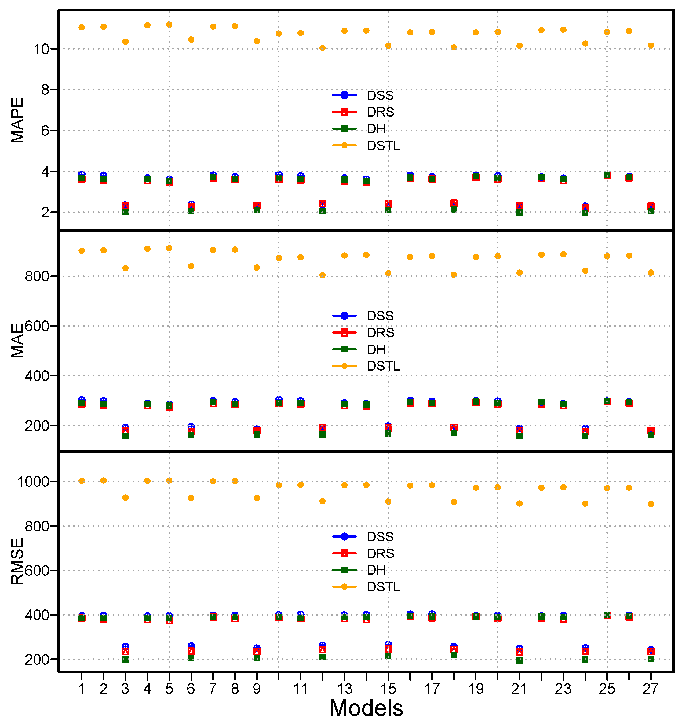
Graphical representations of the performance measures for all 108 models are shown in
Figure 3, for MAPE (top), MAE (center), and RMSE (bottom). From these plots, we can see that the proposed decomposition methods produce the highest accuracy (MAPE, MAE, and RMSE) when compared with the considered benchmark decomposition method. Within the proposed decomposition methods, the DH obtained the highest accuracy. In the same way, the obtained best models for each decomposition method’s mean errors are also plotted in
Figure 4. It can be seen that
DH
,
DH
,
DH
, and
DH
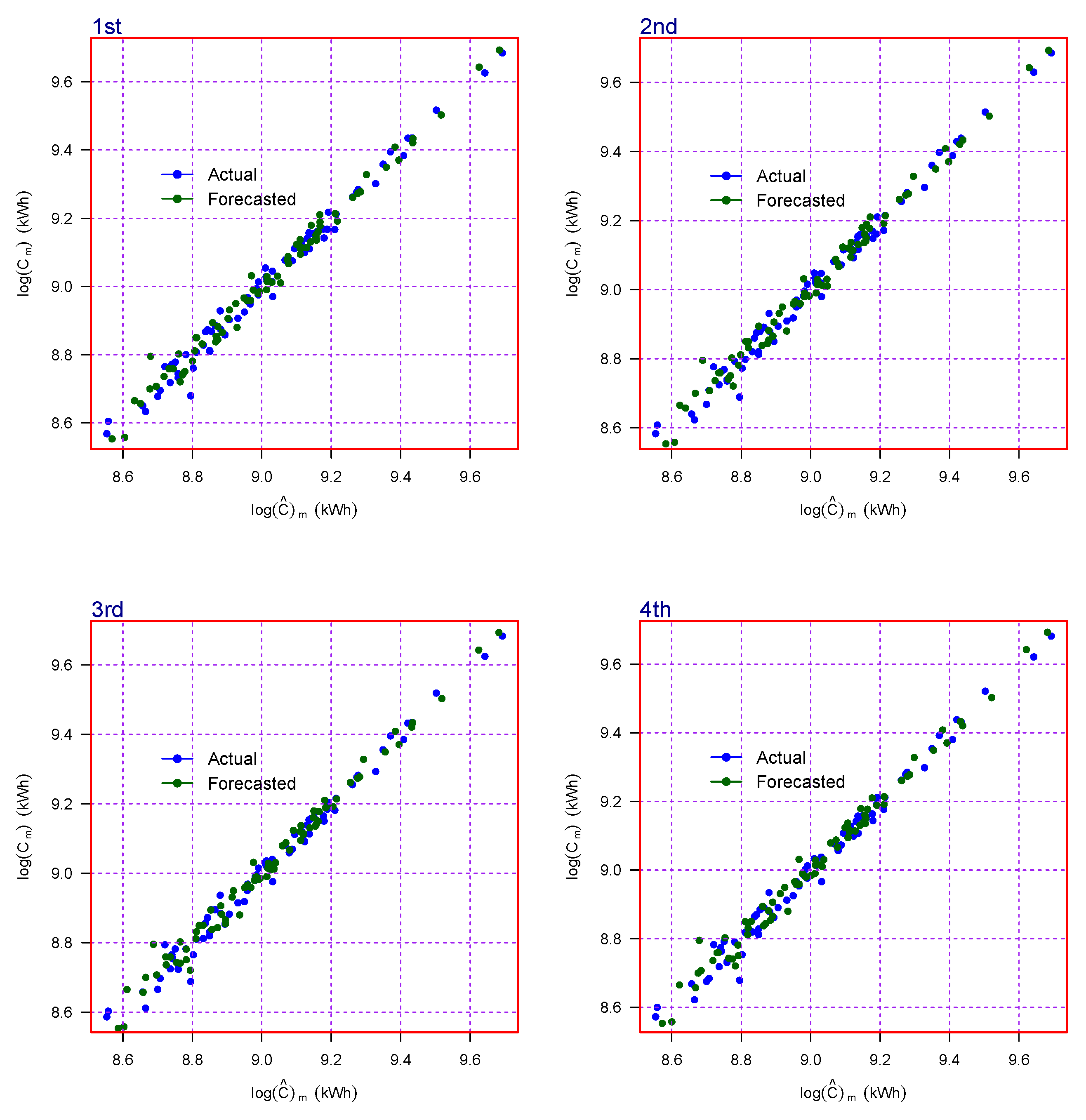
outperform the others. In addition, the correlation plots of the four best models out of the best 12 models in the first selection are shown in
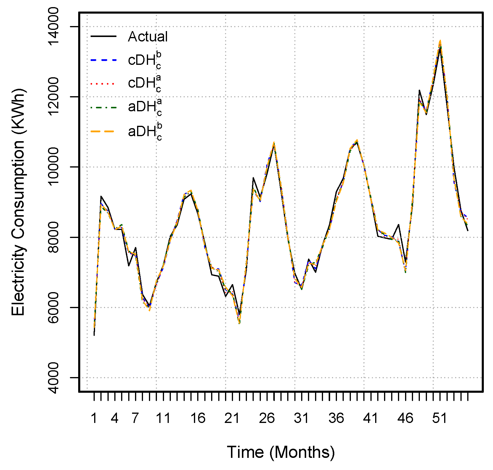
Figure 5. From this figure, we can see that the best model has the highest CORR values and shows a significant correlation between the actual and forecast values. In addition, the original and forecast values for the four best models are shown in
Figure 6.
Figure 6 shows that the best model’s forecasts follow the observed consumption very well. Therefore, from the descriptive statistics, statistical test, and graphical results, we can conclude that the proposed forecasting methodology is highly accurate and efficient for monthly electricity consumption forecasting. Additionally, the proposed decomposition methods have high accuracy and result in efficient forecasts when compared with the considered benchmark method. Within the set of proposed decomposition methods, the DH method produces more precise forecasts when compared with the alternatives.
4. Discussion
According to the results (descriptive statistics, statistical test, and graphical analysis), the conclusion is that the final best models for forecasting the monthly electricity consumption are
DH
,
DH
,
DH
, and
DH
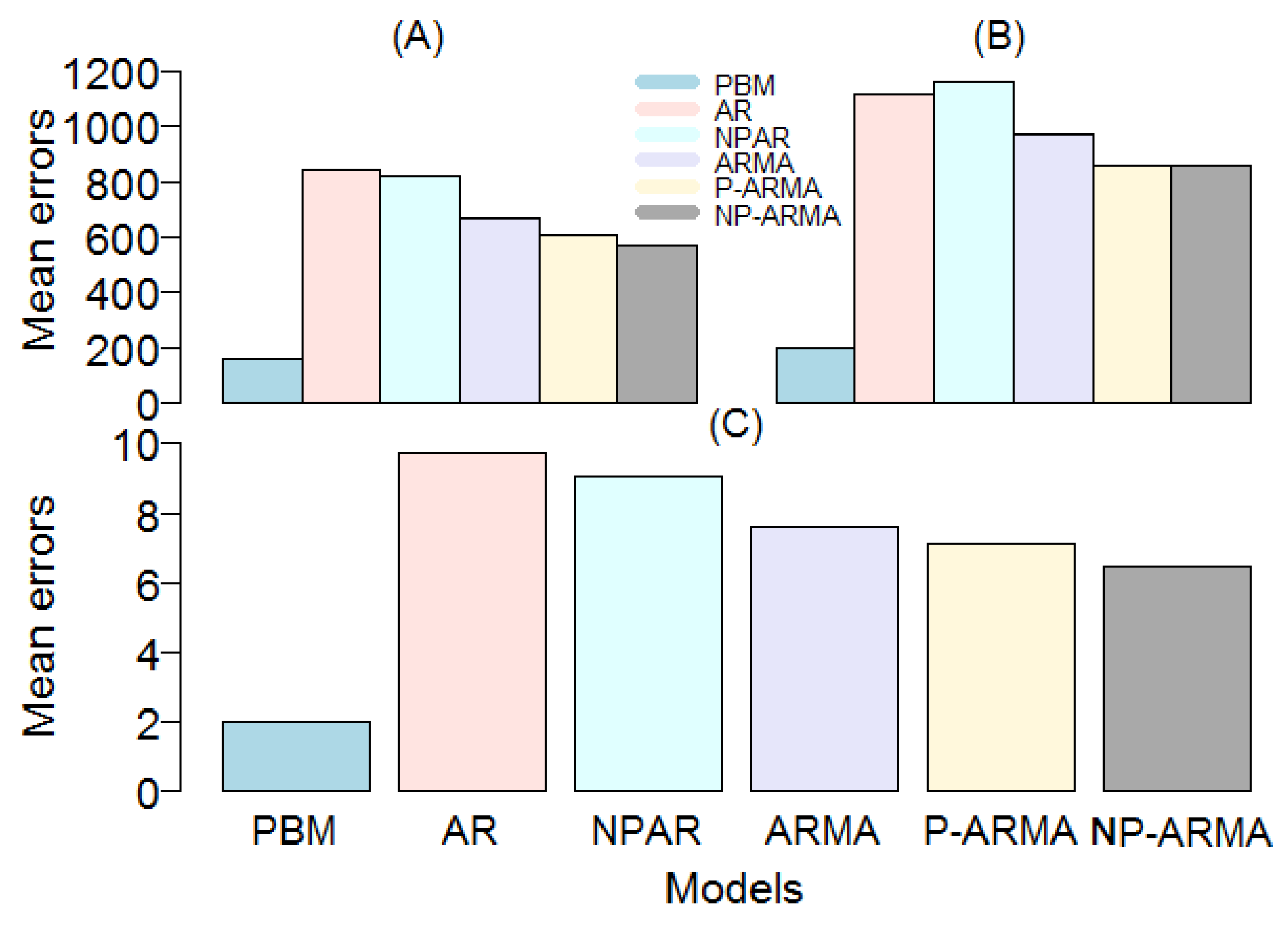
. It is important to note that the reported accuracy measures (MAPE, MAE, and RMSE) in this study are relatively lower than those mentioned in other research articles relating to their best models. For instance, an empirical comparison of the best models proposed in this paper with other researchers’ proposed models is presented numerically in
Table 6 and graphically in
Figure 7. As can be seen in both presentations, the proposed final supermodel in this study produces comparatively significantly smaller mean errors. For example, the two best proposed models (NP-ARMA and P-ARMA) of [
15] were applied to this work’s dataset, and their accuracy measures (MAPE, MAE, and RMSE) were obtained and shown to be significantly higher than those of our best models. In another work, Ref. [
48], the best proposed model (ARIMA (3,1,2)) used the current study dataset and obtained accuracy measures (MAPE, MAE, and RMSE) that are also comparatively higher than those of our best models. In the same way, we also compared the results of our best model with two standard time series models: the linear and nonlinear AR models. The results show that the best model proposed in this paper is significantly better than the time series models considered. Additionally, to confirm the superiority of the proposed best model mentioned in
Table 6, we performed a statistical test using the DM on each pair of models. The results (
p-values) of the DM test are reported in
Table 8, showing that the proposed models among all other works and the standard time series (AR and NPAR) models are outperformed by our best model at the 5% significance level. To conclude, based on all of these results, the accuracy of the proposed forecasting methodology is comparatively high and efficient when compared with all considered competitors.
5. Conclusions
In this study, we aim to provide accurate and efficient electric power consumption forecasts and propose a novel forecasting methodology based on the decomposition and combination of methods for forecasting monthly electric power consumption. For this purpose, we first decompose the power consumption time series into three new subseries: the long-term trend, the seasonal component, and the stochastic component, using the three proposed decomposition methods. Then, to forecast each subseries, all possible combinations are considered using three standard time series models: the linear autoregressive model, the nonlinear autoregressive model, and the autoregressive moving average model. The proposed methodology was applied to data on electricity consumption in Pakistan for the period from January 1990 to June 2020. Four standard accuracy measures (MAPE, MAE, RMSE, and CORR), statistical tests, and a graphical analysis were performed to assess out-of-sample one-month-ahead predictive accuracy. The results show that the proposed methodology is highly effective in forecasting electrical power consumption. Additionally, it is confirmed that the proposed decomposition method outperforms the benchmark decomposition method DSTL, and among the proposed decomposition methods, the hybrid decomposition (DH) method achieves high accuracy. The final combined model produces the minimum mean forecast errors and is relatively better than those reported in the literature and the standard linear and nonlinear time series models. Finally, we believe that the proposed methodology can also be used to solve other real-world forecasting problems that share similar features.
The present study uses only the electricity composition data from Pakistan; it can be extended to the Brazilian reference framework, using the data that were used in [
49]. This will make it possible to broaden the panorama and compare different situations on the subject of energy. Furthermore, the proposed forecasting methodology used only linear and nonlinear time series models; in the future, it will be extended using non-parametric models such as the singular spectrum analysis, machine and deep learning models such as recurrent neural networks, and will support vector regression. This extension will focus on data relating to air pollution in metropolitan Lima, Peru (the same data that was used in [
50]).


 ,
, 


