Thermal Degradation Studies and Machine Learning Modelling of Nano-Enhanced Sugar Alcohol-Based Phase Change Materials for Medium Temperature Applications

Abstract

Thermogravimetric analysis (TGA) was utilised to compare the thermal stability of pure phase change material (D-mannitol) to that of nano-enhanced PCM (NEPCM) (i.e., PCM containing 0.5% and 1% multiwalled carbon nanotubes (MWCNT)). Using model-free kinetics techniques, the kinetics of pure PCM and NEPCM degradation were analysed. Three different kinetic models such as Kissinger-Akahira-Sunose (KAS), the Flynn-Wall-Ozawa (FWO), and the Starink were applied to assess the activation energies of the pure and nano-enhanced PCM samples. Activation energies for pure PCM using the Ozawa, KAS, and Starink methods ranged from 71.10–77.77, 79.36–66.87, and 66.53–72.52 kJ/mol, respectively. NEPCM’s (1% MWCNT) activation energies ranged from 76.59–59.11, 71.52–52.28, and 72.15–53.07 kJ/mol. Models of machine learning were utilised to predict the degradation of NEPCM samples; these included linear regression, support vector regression, random forests, gaussian process regression, and artificial neural network models. The mass loss of the sample functioned as the output parameter, while the addition of nanoparticles weight fraction, the heating rate, and the temperature functioned as the input parameters. Experiment-based TGA data can be accurately predicted using the created machine learning models.

1. Introduction

During the past few decades, with urbanisation and the fast development of populations, the energy demand for space cooling and heating in the construction sector has dramatically increased. It is estimated that around one-third of the world’s energy production is used by the heating industry. As the majority of energy is required for space heating, nations with cold climates are facing substantial energy constraint problems [1]. The average ambient temperature has been raised with the rise in emissions of greenhouse gases, which eventually affects the comfort levels of inside building thermal levels. Hence, passive thermal heating methods are more effective than active thermal methods [1,2,3]. Integrating phase change material (PCM) is one of the best methods of passive heating, which can either reduce or control the building’s interior temperature throughout the day and night. This will help save costs by reducing heat pump running times, improving energy efficiency, etc [4,5]. This helps in finding a solution for the growing energy demands, and the depletion of fossil fuels necessitates the search for such alternate energy sources. However, solar-integrated heat pump systems are becoming the most promising option for space heating applications. However, the imbalance between energy supply and demand has widened due to uneven solar radiation distribution. The most promising approach to closing this gap is to incorporate thermal energy storage (TES) systems into solar thermal systems [6]. Anand et al. [2] conducted an experiment to investigate the effect of the loop heat pipe thermal management system technology on the regulation of the temperature of low-concentrated solar photovoltaic cells. Because it is a passive thermal management approach that does not require the use of any electricity, the phase-change material (PCM)-based solar photovoltaic thermal management method has attracted great interest from researchers [2].

A thermal energy storage (TES) system is a significant method for ensuring a constant supply of energy, which ultimately results in an improvement in both the system’s performance and its consistency. The sensible energy storage system (SESS) and the latent energy storage system (LESS) are the two primary subcategories that make up the TES system. The SESS method occupies more space due to the fact that it mostly depends on the specific heat capacity and mass of the material, whereas the LESS method occupies less volume and majorly depends on the phase transformation enthalpy. Solid–liquid and solid–solid PCM make up the majority of the materials used in LESS because of the fact that they require lower store energy density per unit volume and a higher energy density than liquid–gas phase change materials [7]. Both organic and inorganic PCM materials hold the same principles for energy storage. However, inorganic PCM has superior thermal stability and PCM does not degrade when used in higher temperature applications [8,9].

The two types of PCM materials are organic and inorganic. Organic PCMs are further subdivided into paraffin wax, polymer, alkane, fatty acid, and their eutectic compositions. Specifically, these PCMs excel at storing low-temperature thermal energy (below 120 °C). However, salt hydrates, nitrates, carbonates, chlorides, and metals are all examples of inorganic PCMs that are often used at temperatures below 300 °C (suitable for high temperature applications) [10,11,12]. There are two major classes of inorganic phase change materials: salt hydrates and metals. The volumetric latent heat density, cyclic stability, and thermal conductivity of these materials are all extremely high compared with the organic phase change materials. However, phase segregation and sub-cooling are common in salt hydrates. Since inorganic salts are extremely corrosive, containers must be made of high-quality materials, resulting in a higher cost [13,14,15]. These inorganic PCM salts should offer improved thermal conductivity in particular uses. Inorganic PCMs based on carbon can be utilised to address this issue. The thermal conductivity of inorganic PCM materials can often be enhanced through the use of carbon additive elements. In the past few years, scientists have experimented with a wide range of carbon structured materials, such as nanoparticles made of metal, single- and multi-walled carbon nanotubes [16], and expanded graphite [17]. Space heating, electronic device cooling, refrigeration systems, solar heating, vehicles, food processing and storage, and the space industry are just a few of the many areas where organic latent heat storage materials have been successfully tested [18]. Organic PCMs are advantageous because they do not undergo phase separation; they have a low corrosion resistance with metal containers, and their latent heat of fusion does not change over time [19,20]. Organic PCMs are advantageous in low-temperature applications due to their low melting point. Since organic PCMs have poor thermal conductivity, a greater surface area is required to achieve the necessary heat transfer rate. Since organic PCM has poor thermal conductivity, its application has been restricted. PCM’s thermal conductivity can be improved by incorporating nanometre-sized particles into the base material. Increased thermal conductivity shortens the charge/discharge time period by increasing heat transfer exchange [21]. Because of this, the charge/discharge rate could be increased by applying a minimal quantity of heat. In order to enhance the crystallisation temperature of PCMs, multi-walled carbon nanotubes with high specific surface areas have been proposed as a type of heterogeneous nucleation centre [22,23,24,25]. Among all organic PCM samples, sugar alcohols such as erythritol, xylitol, D-mannitol, Myo-inositol, etc., have become a most promising option for medium temperature applications due to high latent heat of fusion. Jame L. et al. [26] dispersed graphene oxide nanoparticles onto D-mannitol phase change materials to improve their thermal conductivity. The prepared nano-PCM composite could be incorporated into a thermoelectric system for power generation.

Furthermore, a PCM’s thermal stability is an important aspect to consider when using it in thermal energy storage systems. The thermal stability of the PCM can be evaluated with the help of thermogravimetric analysis. Two of the most crucial factors in establishing PCM thermal stability are the rate of degradation and the temperature at which degradation occurs. Experimental TGA measurements, such as temperature versus weight loss at different heating rates, can be used to calculate the degradation kinetics of the chosen PCM samples. TGA studies have shown that temperature plays a significant role in the reaction rate of any given composition. Changes in reaction rate as a function of temperature can be accessed through the activation energy. However, this evaluation is essential for forecasting the thermal stability of nano-enhanced PCMs. Many different kinetic models can be used to study the thermal degradation of organic and inorganic materials using non-isothermal TGA data. There are two primary ways to study kinetics: model fitting and model-free. One or more kinetic models are fitted, and from those models the best statistical fit is determined. The activation energy and pre-exponential factors may be calculated using the kinetic model that best fits the data. It is common practice to use these models to determine the kinetic properties of specific samples using only a single heating rate. Iso-conventional kinetic methods can be used to address the fundamental drawback of this method, which is that it does not take into account variations in activation energy as a function of the heating rate (also known as model-free kinetic methods). The response model may be estimated with a small number of errors using these methods, and they are also quite easy to implement. Degradation of phase transition materials has been recently studied using iso-conventional kinetic techniques [27]. The thermal degradation kinetics of nano-enhanced solid-solid PCM materials were studied by Venkitaraj et al. [28] using the KAS model. According to kinetic analyses, the activation energy of PCM (Pentaerythritol) lowers as the loading of nanoparticles increases (Al₂O₃). Pure PCM and nano-PCM composites with 0.1 and 1% Al₂O₃ each had an average activation energy of 123, 116, and 98 kJ/mole, respectively. Sun et al. [29] developed the microencapsulated PCM using in situ polymerisation. The pentaerythritol and ammonium polyphosphate (PCM) sample is protected within a shell material in this encapsulated PCM material (i.e., melamine-formaldehyde). The kinetics of deterioration of the encapsulated materials were evaluated using the Kissinger and FWO models. The prepared sample had a maximum activation energy of 151.7 kJ/mol. To investigate the thermal stability of the bio-based PCM, Fabiani et al. [30] used iso-conventional techniques (the Starink and Miura-Maki procedures) (Palm Oil). The computed activation energy for both models is between 48.5–127 kJ and 48.1 −126.7 kJ, respectively. Kinetic analysis suggests the two-dimensional phase boundary reaction model best describes palm oil oxidation. Xiang et al. [31] fused various hollow fibre membranes (polypropylene, polysulfone, and polyvinylidene fluoride) to construct shape-stabilised PCMs. Selected PCM samples’ degradation kinetics were analysed using the FWO technique. At a 50% conversion rate, the activation energy of polypropylene-based PCM was measured to be 99.30 kJ/mol, making it the most energy-intensive PCM.

To achieve certain objectives, such as good thermal stability, less degradation, higher peak holding times, etc., it is important to optimise the relevant parameters during PCM preparation. In addition, the empirical method is commonly employed in the industrial sector to decrease experimental effort [32,33]. Modelling and predicting the performance of a variety of engineering systems has been accomplished by researchers making use of Artificial Intelligence (AI) techniques. Therefore, in order to predict PCM degradation, it was required to undertake an extensive examination of the thermogravimetric analysis of PCM materials, which helps in determining the thermal stability of the material. Therefore, to eliminate the repeated experimentation work on various input conditions, several machine learning models have been effectively used for the prediction of thermal stability of PCM samples [16]. The mass loss of the sample is majorly dependent on the addition of nanoparticles weight fraction, the heating rate, and the temperature functioning as the input parameters [17]. As a result, the overall purpose of employing prediction tools helps in achieving an ideal set of parameters [34].

Support vector regression (SVR), Random Forest (RF), and Artificial Neural Network (ANN) are some of the most popular artificial intelligence models that are used to anticipate output characteristics with a high level of accuracy. These machine learning models have been efficiently employed in various engineering applications to create the nonlinear correlations between the output and input features. [27,28]. Ravi et al. studied DSC results of multi-walled carbon nanotubes (MWCNT) [16], binary eutectic/expanded graphite composite nano-PCMs [17], and nano-encapsulated phase change material (NEPCM) [35] to forecast the thermophysical characteristics of various PCM materials behaviour using an artificial neural network. Recently, machine learning models are effectively implemented to predict the TGA plots of the pyrolysis of the bio mass samples [36]. Wang et al. [37] studied the pyrolytic kinetics of various feedstocks using machine learning approaches. This helped in studying thermal decomposition, a model-free pyrolytic activation energy, using RF machine learning methods. Balasore et al. [38] used a machine learning approach for the prediction of biomass pyrolysis kinetics. Wei et al. [39] studied predicting co-pyrolysis of coal and biomass using machine learning approaches.

From the above analyses of the existing literature, it is apparent that researchers have not yet undertaken a thorough analysis into the thermal stability of the nano-enhanced D-mannitol PCM sample. The main objective of this research is to use various model-free integral kinetic models to evaluate the kinetic characteristics of pure PCM and nano-enhanced PCM samples for medium temperature thermal storage systems. This can be accomplished by performing non-isothermal TGA experiments on pure PCM and nano-enhanced PCMs at different heating rates of 10, 20, 30, and 40 °C/min. This current research is being expanded to include the development of various machine learning models for predicting the stability of pure PCM and nano-enhanced PCMs. The type of PCM, heating rates, and temperature at corresponding conversion rates are all considered as input data. As output data, the mass loss of the corresponding input data set is used. These machine learning models effectively predict experimental outcomes with the highest R² values.

2. Materials and Methodology

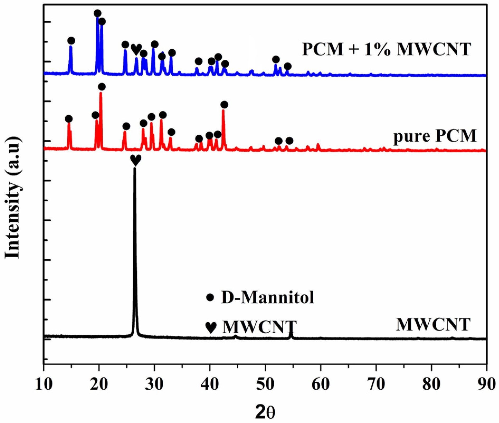
2.1. Sample Preparation and Chemical Stability of Nano PCM Composites

D-Mannitol phase change material, with a melting point in the range of 165–168 °C, was purchased from I lab tech scientific solutions Pvt Ltd. in Trichy, India. The multi-walled carbon nanotube (CNT) was purchased from Royal Scientific Solutions in Trichy, India. It had a nominal diameter of around 4–25 nm, a purity of approximately 98.5%, a specific surface area of approximately 360 m²/g, and an approximate length of approximately 1–15 μm. In order to analyse the crystal structure with the Rigaku Ultima IV, X-ray diffraction was utilised as a technique. The Debye-Scherer relation was used to compute the average crystalline diameter of pure PCM, and the results came out to be 43.1 nanometres. The polymorphic form of pure PCM was shown to be in its b phase when typical peaks were observed at 23.715° and 19.08° (22–1797 JCPDS). For the preparation of nano-enhanced PCM samples, an innovative approach consisting of two steps was chosen. The sample was manufactured by adding MWCNT at various mass fractions (i.e., 0.5 and 1%) using a ball milling technique (High Energy Ball Mill Emax). Sample holders were outfitted with stainless balls, which, due to the centrifugal motions of the balls, ensured consistent mixing of the sample. Following the ball milling procedure, the nanocomposites were subjected to thirty minutes of vigorous ultra-sonication using a probe-type sonicator. The samples were placed on a temperature-controlled flat plate heater so that ultra-sonication could be performed while the substances were still liquid. The thermostat on the heater was set to a temperature of 200 °C, which is considerably higher than the melting point of pure PCM (165–168 °C). After extensive sonification, well-dispersed homogeneous nano-enhanced PCM samples were generated. The XRD peaks of the pure PCM, MWCNT, and nano-enhanced PCM samples are shown in Figure 1. The XRD test of the 0.5% MWCNT-based PCM sample was carried out, and the results showed that there were neither any new peaks nor any notable peak shifts when compared to the XRD spectra of pure PCM. This leads one to believe that there is no significant change in the crystal structure of pure PCM following the dispersion of MWCNT.

The FT-IR was used to investigate how well pure PCM and MWCNT were compatible from a chemical perspective (Make: FT-IR, NIR, and FIR Spectroscopy, PerkinElmer Frontier). The FT-IR spectra of PCM nano composites are shown in Figure 2. After analysing the spectra, it was discovered that the characteristic bands of pure PCM were located at 3280 cm⁻¹, 2942 cm⁻¹, 1386 cm⁻¹, 1078 cm⁻¹, 942 cm⁻¹, 876 cm⁻¹, and 723 cm⁻¹. The stretching frequency of O-H is denoted by the vibrational spectra at a wavelength of 3280 cm⁻¹, with a transmittance percentage of 58.49%. A vibrational peak at 2942 cm⁻¹ with a transmittance of 74.85% was assigned to the stretching frequency, also known as the strong band, for the CH₃, CH₂, and C-H functional groups. The bending vibration of CH₃, CH₂ (medium), and stretching bands were observed in the finger print region at 1386 cm⁻¹ and 1078 cm⁻¹, respectively. At 723 cm⁻¹, 876 cm⁻¹, and 942 cm⁻¹, there was evidence of C-H rocking out of plane, =C-H bending, and C-H bending, respectively. The spectra of nano-enhanced PCM samples showed the same distinctive peaks as those of pure DM, with the exception of a very small shift in transmittance value. It is possible that the physical mixing of the additives in the pure PCM caused these modifications. In addition, the spectra of the nano-augmented PCM showed only modest shifts throughout the whole spectrum, which demonstrates that there was no chemical disintegration in the PCM as a result of the addition of MWCNT. It was clear from the comparison of the FTIR spectra that the composites were chemically inert and could be utilised in LHES on a long-term basis.

2.2. Thermogravimetric Analysis of Nano-PCM Samples

2.2.1. Model-Free Kinetic Methods

A single-step kinetic equation is commonly used to examine the thermal degradation of solid-state reactions.

$$\frac{d\alpha }{dt}=k\left(T\right)·G\left(\alpha \right)$$

(1)

where, α is denoted as conversion of reaction rate, $k \left(T\right)$ is known as reaction rate constant, and $G\left(\alpha \right)$ is defined as a reaction model relevant to the reaction mechanism. Here, the conversion of reaction rate α can be determined by following Equation (2).

$$\mathsf{\alpha }=\frac{\left(m_i-m_{\alpha }\right)}{\left(m_i-m_f\right)}$$

(2)

where $m_i$ is known as the initial mass of the nano-PCM sample, $m_{\alpha }$ mass of the sample at reaction temperature, and $m_f$ is known as the final residual mass of the PCM sample after complete decomposition. The following is the Arrhenius expression stated as a kinetic rate equation with respect to conversion accounting:

$$K\left(T\right)=A·e^{\left(\frac{-E_a}{R_g .T}\right)}$$

(3)

Equation (4) can be obtained by substituting Equation (3) into Equation (1)

$$\frac{d\alpha }{dt}=A·e^{\frac{-E_a}{R_g\times T}}·G\left(\alpha \right)$$

(4)

where the T, $E_a$, and $R_g$ are known as absolute temperature (K), activation energy (kJ/mol), $\beta$ is known as heating rate (K/min) and universal gas constant (Jk⁻¹ mol⁻¹).

A linear increase in temperature with respect to time is observed in non-isothermal conditions;

$$\frac{dT}{dt}=\beta$$

(5)

Equations (4) and (5) can be combined to obtain the following Equation (6)

$$\frac{d\alpha }{dT}=\frac{A}{\beta }· e^{\frac{-E_a}{R_g\times T}}·G\left(\alpha \right)$$

(6)

The above equation can be expressed as an integral, as follows:

$$f\left(\alpha \right)={{\displaystyle \int }}_0^{\alpha }\frac{d\alpha }{G\left(\alpha \right)}=\frac{A}{\beta }{{\displaystyle \int }}_{T_o}^T{e}^{\frac{-E_a}{R_g .T}} dT=\frac{A{E}_a}{\beta R_g}. p\left(z\right)$$

(7)

$p\left(z\right)$ is a temperature integral that is approximated by the numerical approach.

Model fitting and iso-conversional methods are both used to estimate kinetic parameters in non-isothermal thermogravimetric analysis. In order to estimate the kinetic parameters, the model-free method is the most commonly employed approach. The iso-conversional approach yields kinetic parameters with a constant degree of conversion at a constant heating rate. As a result, the iso-conversional method did not require any prior knowledge of kinetic reactions, in which the rate of reaction rate is solely dependent on the degradation temperature of the PCM sample. Differential or integral approaches can be used to obtain the iso-conversional method. FWO, KAS, and Starink methods are the most often used integral methods for determining kinetic parameters.

2.2.2. Kissinger–Akahira–Sunose (KAS)

Kissinger (Kissinger 1957), as well as Akahira and Sunose (Akahira and Sunose 1971), proposed an iso-conversional integral model-free method known as the KAS [40]. KAS employs a simple approximation of the exponential integral, also known as Doyle’s approximation, i.e., $\mathit{p}\left(\mathit{z}\right)\mathbf{=}{\mathit{z}}^{\mathbf{-}\mathbf{2}}\mathbf{\times }{\mathit{e}}^{\mathbf{-}\mathit{z}}$.

$$\ln \left(\frac{\beta }{T^2}\right)=\ln \left[\frac{A\times E_a}{R_g\times g\left(\alpha \right)}\right] -\frac{E_a}{R_g\times T}$$

(8)

Plotting $\mathbf{ln}\left(\frac{\mathit{\beta }}{{\mathit{T}}^{\mathbf{2}}}\right)$ $\mathit{V}\mathit{s} \frac{\mathbf{1}}{\mathit{T}}$ on a graph can be used to determine the activation energy (${\mathit{E}}_{\mathit{a}}$) at each conversion. The slope of the plot at each conversion can be used to estimate the activation energy of the prepared samples.

2.2.3. Flynn-Wall-Ozawa (FWO)

Ozawa (Ozawa 1965) and Flynn and Wall (Flynn and Wall 1966) discovered the FWO kinetic method [41]. It is an integral iso-conversional technique for the computation of activation energy that uses the linear Doyle approximation instead of the temperature integral (Equation (9)), i.e., $\ln \left(p\left(z\right)\right) \approx -5.331-1.052z$.

$$\ln \left(\beta \right)=\ln \left[\frac{A\times E_a}{R_g\times g\left(\alpha \right)}\right]-1.0516\times \frac{E_a}{R_g\times T}$$

(9)

The activation energy ($E_a$) can be determined by plotting the graph of $\ln \left(\beta \right)$ versus $\frac{1}{T}$ at each conversion. The activation energy of the prepared samples can be calculated from the plot slope at each conversion.

2.2.4. Starink Method

The activation energy is estimated using the Starink approach [42], which is similar to the KAS and FWO methods. The activation energy is represented as follows.

$$\ln \left(\frac{\beta }{T^{1.8}}\right)=C_s -1.0037\times \frac{E_a}{R_g\times T}$$

(10)

Plotting the graph of $\ln \left(\frac{\beta }{T^{1.8}}\right)$ versus $\frac{1}{T}$ at each conversion can be used to determine the activation energy ($E_a$). The plot slope at each conversion can be used to estimate the samples’ activation energy.

2.3. Description of Machine Learning Models

2.3.1. Linear Regression

Linear regression is an old technique for determining the degree of association between two or more characteristics. Once the features (input) and the goal (output) are established, the learning process is executed to minimise the loss function value (such as Mean Squared Error). In regression, the optimal parameters are those that result in the smallest loss. This model is reliable and simplistic nature. Multiple linear regression models can be described in their broadest sense by the expression.

$${\widehat{y}}_p=b_o+{{\displaystyle \sum }}_{j=1}^m{x}_j{b}_j$$

(11)

where ${\widehat{y}}_p$ is the predicted outcome, $x_j$ is the selected features, and $b_o and b_j$ are denoted as coefficients of the regression model.

The model is used to find good fits for several linear equations relating the mass loss of the nano-enhanced PCM sample to the specified parameters. The connection between characteristics and mass loss of the PCM sample is convoluted and nonlinear. For this reason, original characteristics of varying polynomial degrees are used to generate polynomial features with the goal of improving the prediction accuracy of the linear regression model [43].

2.3.2. Support Vector Machine

Extending the functionality of support vector machines to regression issues with non-conventional kernels, including polynomial, linear, and radial basis functions. The kernel function is a technique for processing raw data and transforming it into the desired format for further analysis. The radial basis function is a generic kernel that can be applied to any dataset without any prior information. It is critical in small-sample learning that the model’s error margin be minimised, while its generalisation potential be maximised; the SVR approach can accomplish both of these goals. The error-fitting threshold SVR is constructed as follows:

$$R_{SVM}\left(\omega ,a, {\phi }_1,{\phi }_2\right)=\frac{1}{2}{||\omega ||}^2+C_{SVM}\frac{1}{N}{{\displaystyle \sum }}_{i=1}^{m}L\left({\phi }_1,{\phi }_2\right)$$

(12)

$$\mathrm{Subjected} \mathrm{to} \left\{\begin{array}{c}{y}_j-\omega {\tau }_{SVM}\left(x_j\right)-a\le \sigma +{\phi }_1\\ \omega {\tau }_{SVM}\left(x_j\right)+a-y_j\le \sigma +{\phi }_2\\ {\phi }_1,{\phi }_2\ge 0 j=1\dots N\end{array}\right.$$

where $||\omega ||$ is represented as a regularization term, ${\tau }_{SVM}$ is termed as a high dimensional space. The error penalty factor known as $C_{SVM}$ is utilised in the process of determining the optimal trade-off between the regularisation term and the empirical risk. The ${\phi }_{SVM}$ loss function is the one that is equivalent to the approximation precision of the training data point. ${\phi }_1 and {\phi }_2$ are known as loss functions at plane 1 and plane 2. N represents the number of data points. $\sigma$ denotes the variance of the data points. $x_j$ and $y_j$ are termed as input and output parameters.

2.3.3. Random Forest Regression

Random forest (RF) is an ensemble classifier, put to use in the process of conducting analysis on TGA data. The training step of random forest involves the creation of many decision trees, which are then followed by the generation of class labels based on which options received the greatest number of votes. A decision tree stands for a collection of constraints or conditions that are hierarchically organized and carried out in the correct order, beginning at the tree’s origin and progressing outward until they reach the tree’s final node or leaf. When compared with artificial neural networks, the most significant benefit of utilising a hierarchical tree structure is that the structure is visible, which makes it much simpler to understand. To construct the DT from a collection of input datasets, an evaluation measure is applied to each evidential attribute to boost the internode’s level of variability. To obtain the DT, multiple regressions on the dataset, as well as recursive partitioning of the dataset, are utilised. The technique for data splitting is carried out in an iterative fashion, beginning at the root node and continuing until an established termination condition is met. Only specified terminal nodes or leaves are included in the scope of application for a simple regression model. To boost the tree’s generalisation capacity, reduce its structural complexity. When pruning, the total occurrences in a node can be considered. The method known as random forest is one that gathers the results of multiple decision trees into a collective pool and then chooses the most optimal one from among those pools.

RF achieves a high level of regression accuracy and is able to deal with outliers and noise in the data. The use of RF is justified by the fact that it is robust to overfitting and has shown promising regression outcomes in previous studies [44]. The random forest regression is given a sample that has already undergone pre-processing consisting of n samples. Through the utilisation of numerous feature subsets, RF generates n distinct trees. Each tree generates a regression result, and the outcome of the overall model is dependent on the vote of the majority of the trees. The class with the highest total number of votes will be the one to receive the sample. From the literature [44], it is clear that the RF regression model outperforms the decision tree model for such data. The RF has a higher accuracy than the decision tree and there is less of a danger of overfitting the data. Furthermore, it has outperformed other classifiers because it is easy to interpret, non-parametric, and performs well on a large dataset.

2.3.4. Gaussian Process Regression

For nonlinear problems, the non-parametric Gaussian process method is used. It treats all input and output data as though they came from a Gaussian distribution by employing random variables. The Gaussian process, when fed into the training dataset, provides distributions for all realisable functions. Therefore, there is no upper limit on the number of variables that can be employed in a Gaussian process, and this number can be expanded in proportion to the number of datasets used for training. Definition: GPR is a Gaussian process with the mean function m$\left(\dot{z}\right)$ and the kernel function k$\left(\dot{z},\dot{z}\prime \right)$.

$$GR\left(\dot{z}\right)=\mathrm{GPR} \left(\mathrm{m}\left(\dot{z}\right),\mathrm{k}\left(\dot{z},\dot{z}\prime \right)\right)$$

(13)

The central tendency of GR is represented by the variable m$\left(\dot{z}\right)$. The following is a relationship between the values of the test input $\left(\dot{x}\right)$ and the test output $\left(\dot{y_p}\right)$:

$$\dot{y_p}=\mathrm{GR}\left(\dot{z}\right)+\mathsf{\chi }$$

(14)

here, χ is known as the noise of the independent variable. It is represented by a distribution with a mean equal to zero and a standard deviation of ${\phi }_n$, and its definition is as follows:

$$\mathsf{\chi }=\mathrm{Y}\left(0,{\phi }_n^2\right)$$

(15)

A minimal confidence formula is applied to the dataset that is used as a sample. The formula is as follows:

$$\mathrm{J}\left(y|I\right)=\mathrm{Z}\left(y|I,{\phi }_n^{2}K\right)$$

(16)

$$\dot{\mathrm{Y}}={\left[{\dot{Y}}_1,{\dot{Y}}_2,{\dot{Y}}_3,\dots \dots \dots {\dot{Y}}_n\right]}^T$$

(17)

$$\mathrm{g}={\left[GP\left({\dot{z}}_1\right),GP\left({\dot{z}}_2\right),GP\left({\dot{z}}_3\right)\dots \dots \dots GP\left({\dot{z}}_n\right)\right]}^T$$

(18)

The distribution that the predictive dataset follows can be expressed as:

$$\mathrm{J}\left({\dot{Y}}_s|\dot{z},{\dot{z}}^{\text{'}},\dot{Y}\right)=\mathrm{Z}\left({\sigma }_s,{\phi }_s^2\right)$$

(19)

$${\sigma }_s={\complement }_{s,n}{\left({\complement }_n+{\phi }_n^{2}I\right)}^{-1}\dot{Y}$$

(20)

$${\phi }_s^2={\complement }_{ss} -{\complement }_{s,n}{\left({\complement }_n+{\phi }_n^{2}I\right)}^{-1}{\complement }_{M,s}$$

(21)

where ${\sigma }_s$ indicates the mean value of the posterior Gaussian process, ${\phi }_s^2$ the covariance matrix of the prediction data set, ${\complement }_n$ = k (x, x), ${\complement }_{s,n}$ = k ($x^{*}$, x), ${\complement }_{M,s}=\mathrm{k} \left(\mathrm{x}, x^{*}\right),$ and ${\complement }_{s,s}$ = k ($x^{*}$, $x^{*}$). The terms $\complement$ are known as the covariance matrix that connected the training and test data, and $\dot{x}$ is the training dataset. The matrix M × M is represented by I.

2.3.5. ANN Modelling

Simplified nonlinear computational and mathematical models, such as artificial neural networks, are capable of resolving a wide range of engineering challenges. When it comes to predicting experimental outcomes, neural networks have become the most common strategy, with greater performance than older methods. An ANN model mainly consists of an input layer, a hidden layer, and an output layer. The number of neurons in the input layer and output layer is equal to the number of input and output parameters. Connecting processing elements via weighted linkages is common in neural networks. A weighted incoming connection is used for each processing element. The weights and biases of each neuron are changed to train the network structure in an appropriate learning approach. The training continues until the root mean square error is at its lowest. Changing the network’s weights and bias will help lessen the discrepancy between predicted values and actual values. To construct the network, the equation shown below is effectively employed.

$$F\left(H_n\right)=\mathrm{Logsig} (\mathrm{or}) \mathrm{Tan}\mathrm{sig} ({{\displaystyle \sum }}_{j=0}^n\left(W_{ij}\times Z_i\right)+b_j)$$

(22)

In the current ANN structure, the input neuron receives the total amount of information from the input data, which is denoted by the letter $Z_i$. According to the equation, $W_{ji}$ represents the connection weight between the input layer and the hidden layer, and $b_j$ represents the bias of each hidden neuron. $W_{jk}$ and $b_k$, on the other hand, denote the weight connections between the hidden layer and the output layer, and the bias, respectively. The basic structure of an ANN network is shown in Figure 3.

$${\mathrm{O}}_{\mathrm{k}}={\displaystyle \sum }_{\mathrm{k}=0}^{\mathrm{n}}\left({\mathrm{W}}_{\mathrm{jk}}\times {\mathrm{H}}_{\mathrm{n}}\right)+{\mathrm{b}}_{\mathrm{k}}$$

(23)

The anticipated output of each output neuron (O_k) may be determined using Equation (23). The Tansig or Logsig activation function is used between the input and hidden layers, and the purelin activation function is used between the output and hidden layers. The number of neurons present in the hidden layer is critical for the predictability of the network. If there are too few neurons in the hidden layer, the precision of the results will be poorer, whereas if there are too many neurons, the results would be unfair. As a result, it is necessary to optimise the number of neurons in the hidden layer. The optimal neurons are calculated with the help of Equation (24) [16]. The optimal neurons found by solving this equation cannot be considered to be the ultimate solution. The neuronal independence test is carried out with a sufficient number of neurons, falling somewhere within the optimal range.

$${\mathrm{H}}_{\mathrm{n}}=\frac{\mathrm{Input}+\mathrm{Output}}{2}+\sqrt{\mathrm{Train} \mathrm{data}}$$

(24)

Normalisation of input and output data is essential to increase the accuracy of results. With this normalisation, accuracy and convergency time could be improved. Within the range of 0 to 1, the input and output data are normalised. Use the following equation to determine data normalisation.

$$Z=\frac{\left(Z_i-Z_{min}\right)}{\left(Z_{max}-Z_{min}\right)}\left(H-L\right)+L$$

(25)

The L and H denote the normalized data set’s lower and higher limit values. $Z_{min}$ and $Z_{max}$ are known as the minimum and maximum values of the dataset. $Z_i$ is known as the selected data point.

3. Results and Discussion

3.1. Thermogravimetric Analysis of Prepared Nano-Enhanced PCM Samples

Figure 4a–c show the thermogravimetric curves of D-mannitol PCM with different multi-walled carbon nanotubes weight fractions (0, 0.5, and 1%) at heating rates of 5 °C/min, 10 °C/min, 15 °C/min, and 20 °C/min. The results of the TGA are presented as a percentage of the PCM samples’ weight loss as a function of the temperature. The PCM samples were heated from 40 to 700 °C at a variety of different heating speeds. Experiments were conducted with an initial sample size of 5 ± 0.5 mg in an alumina sample pan under a nitrogen environment, with the gas flow rate set at 60 ml/min. From the results, it can be seen that no samples were degraded, and the overall weight loss was found to be negligible (less than 2%) during the phase transition zone. The temperature area of D-mannitol (below 200 °C) indicates that D-mannitol was thermally stable for the application of energy storage in the temperature range of its phase transition. When the pace of heating was increased, the experiment revealed that the temperature at which the decomposition process begins was significantly elevated. As the temperature rises, an examination of the TG curves revealed a progressive decomposition pattern that occurred in a single step at each new temperature. The melting process that resulted from heat degradation was responsible for this decomposition, which may be traced back to the original substance. The rate of weight loss also varied, but it was often slower at the beginning stages of decomposition. The rate of weight loss was also variable. Chemical reactions, the release of species that were adsorbed, and breakdown are the three processes that may be singled out as the causes of the weight loss that occurs during thermal cycling.

The thermogravimetric analysis (TG) results of pure D-mannitol are displayed in Figure 4a, which compares the effects of several heating rates. When heated at a rate of 5 °C per minute, the pure PCM sample began to degrade, albeit at a slower pace at first; however, at about 248.87 °C, there was only a weight loss of less than 5%. This initial weight loss was primarily attributable to the loss of PCM as it evaporated. The rate of weight loss accelerated fast above 260 °C, showing weight losses of 20%, 40%, 60%, and 80% at temperatures of 271.06 °C, 284.99 °C, 300.94 °C, and 312.83 °C, respectively. At temperatures of 285.33 °C, 297.21 °C, 317.25 °C, and 329.14 °C, respectively, weight losses of 20%, 40%, 60%, and 80% were observed when the heating rate was increased to 10 °C per minute. In the situation of TG that was carried out at a heating rate of 15 °C/min, weight losses of 20%, 40%, 60%, and 80% were seen at temperatures of 295.538 °C, 311.49 °C, 331.53 °C, and 347.52 °C, respectively. Again, when the rate of heating was increased to 20 °C per minute, these weight losses were recorded at temperatures of 311.87 °C, 327.83 °C, 349.93 °C, and 365.87 °C, respectively.

Figure 4 displays the thermogravimetric data that were collected for PE combined with 0.5% MWCNT at a variety of heating rates (b). When the sample was heated at a rate of 5 °C/min, it was seen that the addition of 0.5% of the weight fraction of MWCNT had very little effect on the deterioration at the beginning of the process. At a temperature of 229.91 °C, there was still a loss of weight of less than 5%. However, at temperatures higher than 260 °C, the degradation of D-mannitol plus 0.5% MWCNT occurred at a pace that was slightly faster than that of pure PE. The thermogravimetric analysis (TG) results of D-mannitol combined with 0.5% MWCNT indicated weight losses of 20%, 40%, 60%, and 80% at temperatures of 264.80 °C, 279.17 °C, 293.54 °C, and 305.86 °C, respectively. The heating rate used was 5 °C/min. When the rate of heating was increased to 10 °C per minute, weight losses of 20%, 40%, 60%, and 80% were seen at temperatures of 279 °C, 293.54 °C, 309 °C, and 324 °C, respectively. In the situation of TG carried out at a heating rate of 15 °C/min, weight losses of 20%, 40%, 60%, and 80% were seen at temperatures of 289.44 °C, 305.86 °C, 324.34 °C, and 338.70 °C, respectively. When the rate of heating was increased to 20 °C per minute, these weight losses were seen at temperatures of 299.70 °C, 322.28 °C, 342.81 °C, and 363.34 °C, respectively.

Figure 4c illustrates the thermogravimetric (TG) curves of D-mannitol with 1% MWCNT at a variety of heating rates. According to the findings, the addition of MWCNT at a weight fraction of 1% caused the sample to undergo degradation a great deal sooner than when it was treated with pure D-mannitol or D-mannitol combined with 1% MWCNT. This is because a higher concentration of MWCNT nanoparticles allows for a more efficient transfer of heat, which led to the observed phenomenon. At a temperature of 244.18 °C, the thermogravimetric analysis (TG) results showed that the sample of pure D-mannitol had lost nearly 10% of its weight. A weight loss of 20%, 40%, 60%, and 80% was recorded at temperatures of 256.58 °C, 271.24 °C, 281.81 °C, and 294.41 °C, respectively. This was also observed when the rate of heating was increased to 10 °C per minute; weight losses of 20%, 40%, 60%, and 80% were seen at temperatures of 268.81 °C, 283.44 °C, 296.05 °C, and 308.67 °C, respectively. In the situation of TG carried out at a heating rate of 15 °C/min, weight losses of 20%, 40%, 60%, and 80% were seen at temperatures of 285.61 °C, 301.31 °C, 316.97 °C, and 330.72 °C, respectively. Again, when the rate of heating was increased to 20 °C per minute, these weight losses were seen at temperatures of 297.27 °C, 322.13 °C, 336.73 °C, and 357.49 °C, respectively. Because of this, it is clear from the previous examination of the TG results that an increase in the heating rate influences both the location of the temperature gradient (TG) curve and the rate of breakdown. The maximum points on the TG curves go upwards toward higher temperatures as a result of the rise in the heating rate.

As an energy barrier, activation energy works against the degrading reaction. As seen in Figure 5, PCM samples show a wide range of conversion rates ($\alpha$). Activation energies of pure PCM, PCM + 0.5% MWCNT, and PCM + 1% MWCNT were estimated in this experiment using iso-conversional methods described by Kissinger Akahira-Sunose, Flynn-Wall-Ozawa, and Starink kinetic models. The activation energy (E) for complete PCM decomposition was determined for various conversion values (0.2 to 0.8). KAS, FWO, and Starink kinetic models are analysed by plotting the plots between $\ln \frac{\beta }{T^2}$ and $\frac{1000}{T}$, $\ln \beta$ and $\frac{1000}{T}$, $\ln \frac{\beta }{T^{1.8}}$, and $\frac{1000}{T}$, respectively. The R² value of the linear fitted lines of developed kinetics models of prepared samples are more than 0.92. Figure 6, Figure 7 and Figure 8 present these plots for pure PCM, PCM + 0.5% MWCNT, and PCM + 1% MWCNT. As previously discussed, the activation energy was obtained by determining the slope of the plots. The calculated activation energies for various conversion values for pure PCM, PCM + 0.5% MWCNT, and PCM + 1% MWCNT are shown in

Table 1. Activation energy values of various PCM samples for developed kinetic models.

Conversion (α)	Activation Energy (Ea) (kJ/mol)
	KAS Method	OFW Method	Starink Method
Pure PCM
0.2	65.89	71.10	66.53
0.3	78.76	83.74	79.40
0.4	76.52	81.74	77.17
0.5	78.36	83.60	79.02
0.6	80.80	86.08	81.47
0.7	74.51	80.25	75.22
0.8	71.79	77.77	72.52
PCM + 0.5% MWCNT
0.2	79.36	84.14	79.97
0.3	86.36	90.97	86.97
0.4	77.64	82.82	78.29
0.5	75.47	80.92	76.15
0.6	70.06	75.90	70.77
0.7	68.74	74.79	69.47
0.8	66.87	73.13	67.62
PCM + 1% MWCNT
0.2	71.52	76.59	72.15
0.3	70.88	76.17	71.54
0.4	68.74	74.27	69.41
0.5	60.35	66.43	61.07
0.6	57.46	63.78	58.20
0.7	55.90	62.43	56.67
0.8	52.28	59.11	53.07

. The average activation energy calculated using the KAS, OFW, and Starink methods for pure PCM sample is 76.12, 81.63, and 76.81 kJ/mol, respectively; for the PCM + 0.5% MWCNT sample, it is 74.93, 80.38, and 75.61 kJ/mol, respectively; for the PCM + 1% MWCNT sample, it is 62.45, 68.40, and 63.16 kJ/mol, respectively. It was found that the estimated activation values for the different models fall into the following order: OFW > Starink > KAS. The results make it abundantly evident that the activation energy calculated using the OFW model is significantly higher than that computed using the other models. From the results, it is also seen that activation energies are changed with respect to each conversion of decomposition. The main reason for the variation in activation energy is due to the non-homogeneous structure of the selected samples, or may be due to the complex reaction mechanism. In the case of pure PCM, the estimated activation energies varied in ranges of 65.89–71.79, 71.52–77.77, and 66.53–72.52 kJ/mol for the KAS, OFW, and Starink methods, respectively. For the PCM + 0.5% MWCNT sample, the estimated activation energies varied in ranges of 79.36–66.87, 84.14–73.13, and 79.97–67.62 kJ/mol for the KAS, OFW and Starink methods, respectively. However, in the case of the PCM + 1% MWCNT sample, the estimated activation energies varied in ranges of 71.52–52.28, 76.59–59.11, and 72.15–53.07 kJ/mol for the KAS, OFW and Starink methods, respectively.

3.2. Kinetic Characterization of Nano Enhanced PCM Samples

D-mannitol PCM degradation kinetics after MWCNT nano-particle addition was investigated using thermogravimetric analysis data. Determining D-mannitol degradation kinetics using a non-isothermal method was carried out because it more closely mimics actual industrial processing conditions. The PCM samples were heated from room temperature to 700 °C at continuous scanning speeds of 5, 10, 15, and 20 °C/min for non-isothermal measurements, and the resulting percentage weight loss was recorded. In this work, the thermal degradation kinetics of D-mannitol with added MWCNT nanoparticles was investigated using iso-conversional techniques. Using the relationship between activation energy and conversion degree, a kinetic analysis of thermal decomposition was performed.

Lower activation energy indicates that the least amount of energy is necessary to break the PCM molecules, which in turn speeds up the rate at which the reaction occurs. According to the findings, it can be shown that the rate of decomposition of PCM is initially lower (that is, at 20% conversion), but then it quickly rises to 60%. This is because the calculated activation energy of PCM has increased from 10% to 60% of the conversion range. The rate of decomposition continues to gradually increase until it reaches a state of rest, at which point it can reach up to 80% conversion. This is due to a slight decrease in the activation energy value. From Table 1, it can be seen that the rate of decomposition of nano-enhanced PCM samples are initially higher (that is, at 20% conversion), but then it sharply decreases up to 80%. The pure PCM sample was analysed, and the activation energy was determined to have an average value of 76.12 kJ/mol. Whereas, the calculated average activation energy values (i.e., using the KAS model) for PCM samples containing 0.5% MWCNT and 1% MWCNT were 74.93 and 62.45 kJ/mol, respectively, which was 1.56% and 17.96% smaller than the activation energy values for the pure PCM sample. Though this drop is rather small at low MWCNT nano-particle weight fractions, it becomes extremely noticeable at large nano-particle weight fractions. These findings demonstrate that MWCNT addition reduces the activation energy of pure PCM. MWCNT nanoparticles not only operate as a textural support that improves surface area, but the are also involved in catalysis, as evidenced by the reduction in activation energy values upon their incorporation. As a result, MWCNT nanoparticles catalyse pure PCM samples, reducing the latter’s activation energy. Chemical reactions simultaneously occur with evaporation, reducing the activation energy required for the former process. Condensation appears to take place in pure PCM, leading to the loss of water and, consequently, mass, as well as the creation of a low volatility condensation product. Thermogravimetric analysis (TG) reveals that in the RT−200 °C operating temperature range, pure PCM and PCM added with 0.5 and 1 wt.% of MWCNT show no appreciable weight loss. At these temperatures, evaporation hardly contributes to the thermal degradation of the samples.

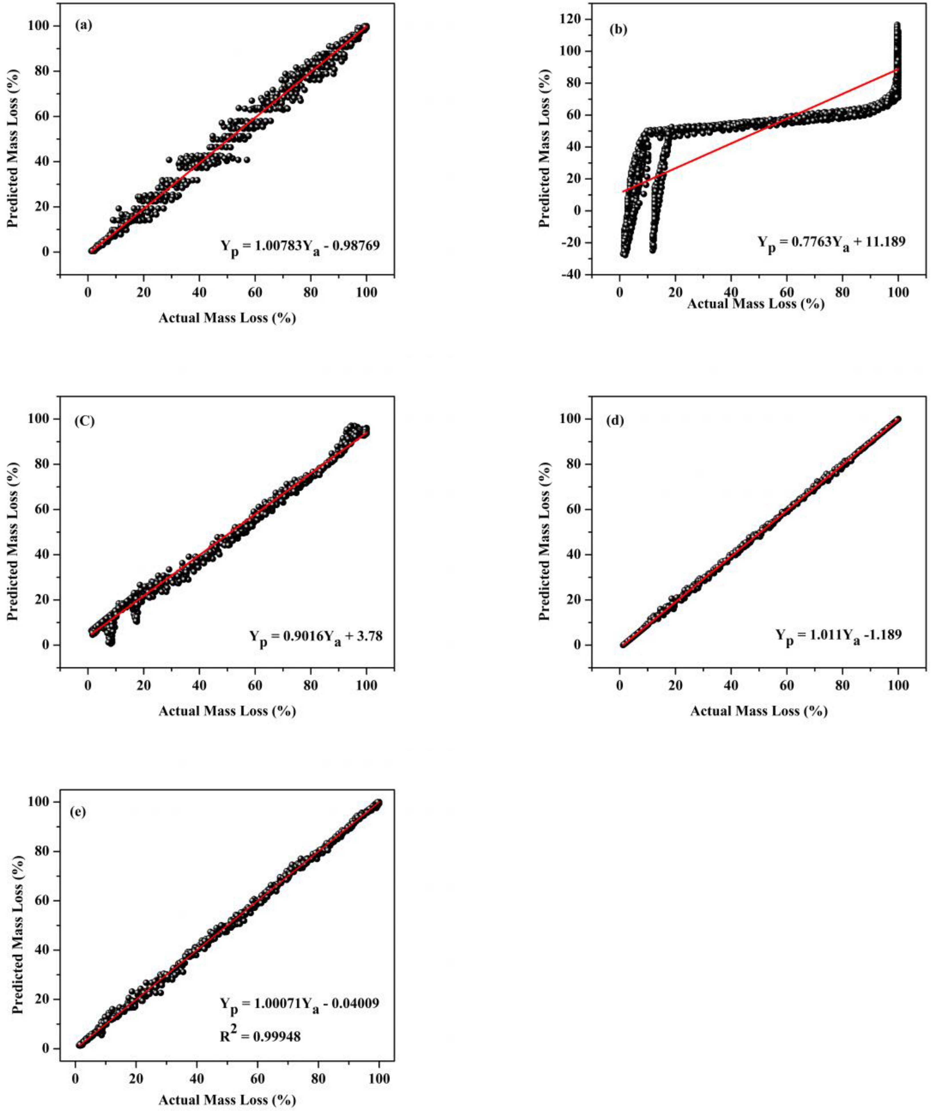
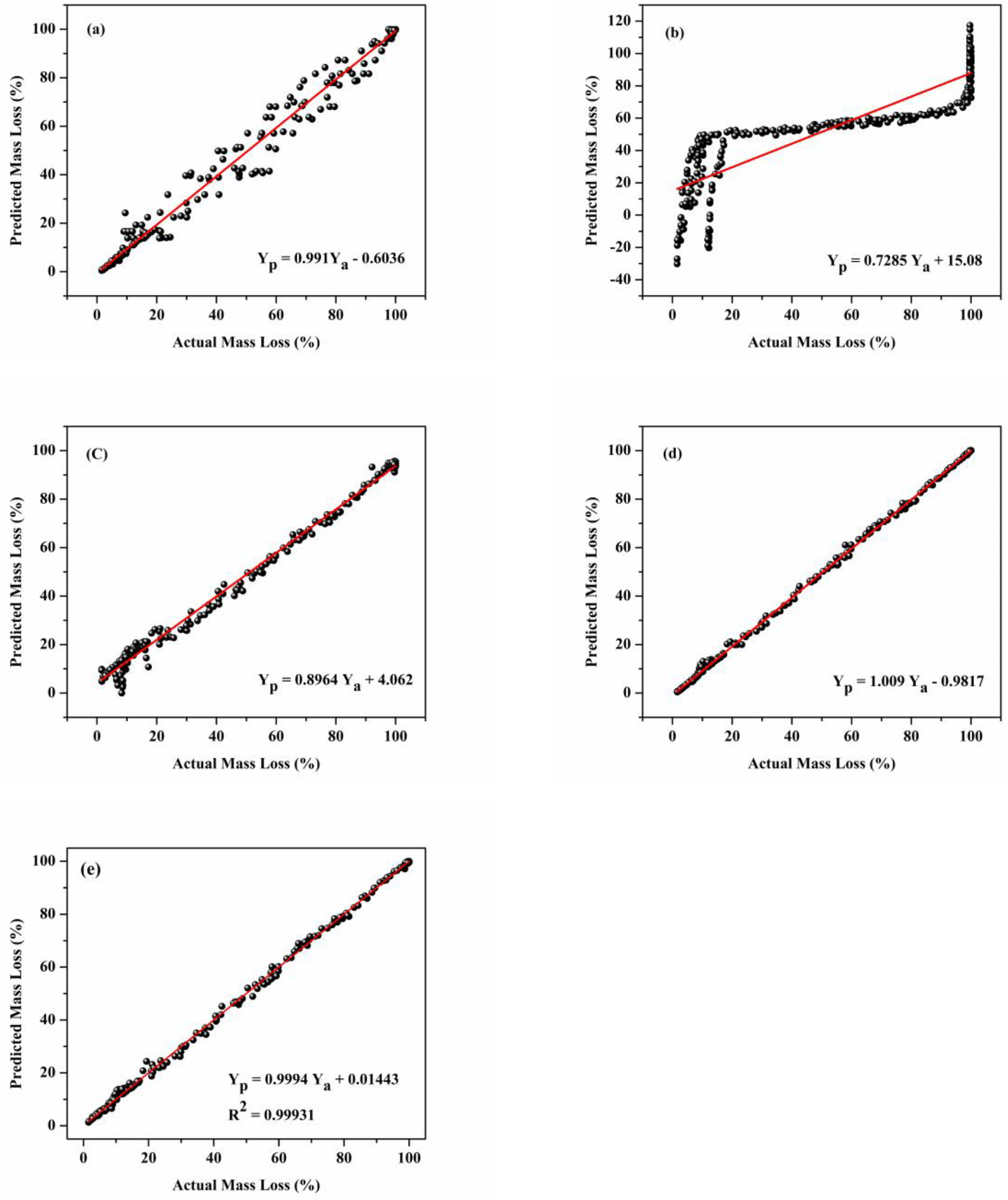
3.3. Machine Learning Modelling of Thermal Degradation of Nano Enhanced PCM Samples

In the present study, the mass loss of the samples of pure PCM and nano-enhanced PCM was anticipated by making use of three distinct characteristics: the weight percent of MWCNT, the heating rate, and the temperature. Python 3.10.5 software was used to construct machine learning models on the basis of experimental data in order to make a prediction about the mass loss of the PCM sample.

3.4. Hyper-Parameter Tuning of Developed Machine Learning Models

Finding the exact values of the hyperparameters is a vital component of developing a successful model, especially for a parameter-sensitive algorithm like a random forest, support vector machine, Gaussian process regression, or ANN model. To find the machine learning model that yields the best results, various hyperparameter settings can be tested. The optimal settings for each model’s hyperparameter values are listed in

Table 2. Hyper-parameter tuning values of developed machine learning models.

Model	Parameter	Value
Support vector machine	kernel	rbf
	degree	3
Random Forest Regression	n-estimators	55
	Min-samples-split	3
	Min-samples-leaf	1
	Max-depth	9
Gaussian Process Regression	Basis function	0
	Sigma	0.143
	Kernel function	Isotropic matern 3/2
ANN	Number of hidden layers	1
	Number of hidden neurons	33
	Activation functions	Tanh, Purelin

. The ANN model makes use of three layers of feed-forward back propagation in its computations. The output neurone reflects the mass loss of the PCM sample, while the input neurones are substituted in for the various factors that were investigated in the experiment (such as weight fraction of the MWCNT, heating rate, and temperature). As an activation function that lies between the input layer and the hidden layer, the hyperbolic tangent sigmoid (tanh) function is utilised. From the literature [16], the tanh function has shown significantly better performance than the sigmoid function. On the other hand, the purelin function is employed in the role of an activation function between the input layer and the hidden layer. The method of finding the optimal number of hidden neurones in the hidden layer consisted of multiple rounds of trial and error. In order to establish which neural network is the most effective for this purpose, a neural independence test was carried out. The results showed that the RMSE and R² values were at their lowest and highest levels, respectively, when there were 33 hidden neurones.

3.5. Comparison of Model Accuracy of Developed Machine Learning Models

The variation of MSE value with respect to the iterations at optimal neural network is shown in Figure 9. Figure 10 indicates the regression plots of optimal network topology. The correlation coefcient (R) values for all data sets are nearly equal to one, as shown in the plots. This indicates that the developed optimum network’s data predictions are consistent with the experimental data.

A scatter plot is an accurate representation of the accuracy of the machine learning models that were generated. The scatter distribution of both experimental and predicted values of various machine learning models is depicted in Figure 11. Alongside the anticipated values of mass loss, a regression diagonal line is presented that connects the experimental data to the expected values. If the scattered points are grouped together in close proximity to the diagonal line, then the model has a high R² value and provides a strong fit. On the other hand, if the points are scattered in a direction that is not perpendicular to the diagonal line, then the model has a lower level of goodness of fit and R² values. When compared to the scatter distribution of the other machine learning models, as shown in Figure 12, the scatter distribution of the Gaussian process regression and ANN machine learning models are more concentrated near the centre line. This can be seen by looking at the distance between the centre line and the scatter distribution. Around the diagonal line, the scatter point distribution of the other machine learning models demonstrates a broad or foggy dispersion. The Gaussian process regression model has the best scatter distribution of points out of all the models because it has the least amount of deviation around the diagonal line.

3.6. Sensitivity Analysis

The root-mean-square error (RMSE) and the correlation coefficient (R²) were employed as performance indicators to measure the model’s accuracy. The best neural structure was found to have an RMSE of 0.8437 and an R² of 0.9998. Similar to how RMSE and R² values were used to evaluate the accuracy of the aforementioned models’ predictions, the remaining machine learning models were also evaluated. The relative RMSE and R² are shown in

Table 3. Sensitivity analysis of developed machine learning models.

Model	Training		Testing		Validation
	RMSE	R2	RMSE	R2	RMSE	R2
Random Forest Regression	2.6325	0.9983	4.2996	0.9957	19.9326	0.9029
Linear Regression	18.6926	0.9162	19.4342	0.9154	20.0745	0.8854
Support vector machine Regression	4.7426	0.9946	4.9398	0.9944	18.9254	0.9113
Artificial Neural Network	0.8437	0.9998	1.0541	0.9997	20.1265	0.9010
Gaussian Process Regression	0.8871	0.9998	1.000	0.9998	1.0632	0.9997

. Table 3 shows that all of the created ML models, with the exception of the linear regression model, have R² values above 0.95. ANN and Gaussian process regression models in machine learning have the highest R² and the lowest RMSE. When compared to the ANN model, the results from the Gaussian process regression model are more promising. For the regression model based on the Gaussian process, the obtained RMSE and R² values were 0.8871 and 0.9998, respectively. According to the data in Table 3, the Gaussian process model best describes the results of the experiments. To a high degree, the results of the Gaussian process regression model match with the results of the experimental testing dataset. Thus, the non-linear relationship between the study’s output and input parameters can be accurately predicted by employing the Gaussian process regression technique.

3.7. Model Accuracy Test

The prediction performance of the developed machine learning models can be determined with the help of the known TGA experimental dataset. The PCM with the 0.5% MWCNT sample was heated at 7.5 °C·min⁻¹ using TGA equipment, and the experimental outcomes of this sample were considered as the validation dataset. The comparison of validated experimental TGA data and machine learning models predicted values are shown in Figure 13. From Figure 13 shows that the Gaussian regression model is well predicted with the lowest RMSE value of 1.0632 and the highest R² value of 0.9997.

4. Conclusions

In this study, TGA analysis of samples of pure PCM and nano-enhanced PCM samples were carried out using a variety of heating rates. In order to evaluate the thermal degradation kinetics of the proposed PCM samples, various degradation kinetic models such as KAS, FWO, and Starink models were employed. Using these kinetic models, the activation energy of the prepared samples was determined. The Ozawa, KAS, and Starink techniques all produced activation energies for pure PCM that varied between 66.53 to 72.52 kJ/mol, 79.36 to 66.87 kJ/mol, and 71.10 to 77.77 kJ/mol, respectively. The activation energies of NEPCM (1% MWCNT) were 76.59 to 59.11, 71.5 to 52.28, and 72.15 to 53.07 kJ/mol. According to the results, it could be observed that the prepared nano-enhanced PCM samples were chemically and thermally stable. In addition, several machine learning models were developed to predict the thermal degradation of the chosen PCM samples. These included linear regression, support vector regression, random forest, Gaussian process regression, and artificial neural network models. The generated models could accurately predict the experimental TGA dataset of PCM samples across a wide range of operating conditions. In summary, the findings of this work add to a better understanding of the thermal degradation that nano-enhanced PCM undergoes when it is used for thermal storage applications.

References

1. Jinshah, B.S.; Ramaraj, B.K.; Kottala, R.K.; Sivapirakasam, S.P. A complete numerical model for low temperature composite form-stable phase change material slab based on dynamically simplified temperature transforming method. Energy Sources A Recovery Util. Environ. Eff. 2021, 1–26. [Google Scholar] [CrossRef]
2. Balasubramanian, K.R.; Jinshah, B.S.; Ravikumar, K.; Divakar, S. Thermal and hydraulic characteristics of a parabolic trough collector based on an open natural circulation loop: The effect of fluctuations in solar irradiance. Sustain. Energy Technol. Assess. 2022, 52, 102290. [Google Scholar] [CrossRef]
3. Jinshah, B.S.; Kottala, R.K.; Balasubramanian, K.R.; Francis, A. Experimental analysis of phase change material integrated single-phase natural circulation loop. Mater. Today Proc. 2021, 46, 10000–10005. [Google Scholar] [CrossRef]
4. Jinshah, B.S.; Balasubramanian, K.R.; Kottala, R.; Divakar, S. Influence of power step on the behavior of an Open Natural Circulation Loop as applied to a Parabolic Trough Collector. Renew. Energy 2022, 181, 1046–1061. [Google Scholar] [CrossRef]
5. Marudaipillai, S.K.; Karuppudayar Ramaraj, B.; Kottala, R.K.; Lakshmanan, M. Experimental study on thermal management and performance improvement of solar PV panel cooling using form-stable phase change material. Energy Sources A Recovery Util. Environ. Eff. 2020, 45, 160–177. [Google Scholar] [CrossRef]
6. Senthilkumar, M.; Balasubramanian, K.R.; Kottala, R.K.; Sivapirakasam, S.P.; Maheswari, L. Characterization of form-stable phase-change material for solar photovoltaic cooling. J. Therm. Anal. Calorim. 2020, 141, 2487–2496. [Google Scholar] [CrossRef]
7. Goud, M. A comprehensive investigation and artificial neural network modeling of shape stabilized composite phase change material for solar thermal energy storage. J. Energy Storage 2022, 48, 103992. [Google Scholar] [CrossRef]
8. Goud, M.; Raval, F. A sustainable biochar-based shape stable composite phase change material for thermal management of a lithium-ion battery system and hybrid neural network modeling for heat flow prediction. J. Energy Storage 2022, 56, 106163. [Google Scholar] [CrossRef]
9. Peter, R.J.; Balasubramanian, K.R.; Kumar, K.R. Comparative study on the thermal performance of microencapsulated phase change material slurry in tortuous geometry microchannel heat sink. Appl. Therm. Eng. 2023, 218, 119328. [Google Scholar] [CrossRef]
10. Luo, J.; Zou, D.; Wang, Y.; Wang, S.; Huang, L. Battery thermal management systems (BTMs) based on phase change material (PCM): A comprehensive review. J. Chem. Eng. 2022, 430, 132741. [Google Scholar] [CrossRef]
11. Karthick, A.; Manokar Athikesavan, M.; Pasupathi, M.K.; Manoj Kumar, N.; Chopra, S.S.; Ghosh, A. Investigation of inorganic phase change material for a semi-transparent photovoltaic (STPV) module. Energies 2020, 13, 3582. [Google Scholar] [CrossRef]
12. Ye, R.; Fang, X.; Zhang, Z. Numerical Study on Energy-Saving Performance of a New Type of Phase Change Material Room. Energies 2021, 14, 3874. [Google Scholar] [CrossRef]
13. Hua, W.; Xu, X.; Zhang, X.; Yan, H.; Zhang, J. Progress in corrosion and anti-corrosion measures of phase change materials in thermal storage and management systems. J. Energy Storage 2022, 56, 105883. [Google Scholar] [CrossRef]
14. Bell, S.; Jones, M.W.M.; Graham, E.; Peterson, D.J.; van Riessen, G.A.; Hinsley, G.; Will, G. Corrosion mechanism of SS316L exposed to NaCl/Na2CO3 molten salt in air and argon environments. Corros. Sci. 2022, 195, 109966. [Google Scholar] [CrossRef]
15. Moreno, P.; Miro, L.; Sole, A.; Barreneche, C.; Sole, C.; Martorell, I.; Cabeza, L.F. Corrosion of metal and metal alloy containers in contact with phase change materials (PCM) for potential heating and cooling applications. Appl. Energy 2014, 125, 238–245. [Google Scholar] [CrossRef]
16. Ravi Kumar, K.; Balasubramanian, K.R.; Jinshah, B.S.; Abhishek, N. Experimental analysis and neural network model of MWCNTs enhanced phase change materials. Int. J. Thermophys. 2022, 43, 11. [Google Scholar] [CrossRef]
17. Kottala, R.K.; Ramaraj, B.K.; BS, J.; Vempally, M.G.; Lakshmanan, M. Experimental investigation and neural network modeling of binary eutectic/expanded graphite composites for medium temperature thermal energy storage. Energy Sources A Recovery Util. Environ. Eff. 2022, 1–24. [Google Scholar] [CrossRef]
18. Png, Z.M.; Soo, X.Y.D.; Chua, M.H.; Ong, P.J.; Suwardi, A.; Tan, C.K.I.; Zhu, Q. Strategies to reduce the flammability of organic phase change Materials: A review. Sol. Energy 2022, 231, 115–128. [Google Scholar] [CrossRef]
19. Saleel, C.A. A review on the use of coconut oil as an organic phase change material with its melting process, heat transfer, and energy storage characteristics. J. Therm. Anal. Calorim. 2022, 147, 4451–4472. [Google Scholar] [CrossRef]
20. Tyagi, V.V.; Chopra, K.; Sharma, R.K.; Pandey, A.K.; Tyagi, S.K.; Ahmad, M.S.; Kothari, R. A comprehensive review on phase change materials for heat storage applications: Development, characterization, thermal and chemical stability. Sol. Energy Mater. Sol. Cells 2022, 234, 111392. [Google Scholar] [CrossRef]
21. Ma, C.; Wang, J.; Wu, Y.; Wang, Y.; Ji, Z.; Xie, S. Characterization and thermophysical properties of erythritol/expanded graphite as phase change material for thermal energy storage. J. Energy Storage 2022, 46, 103864. [Google Scholar] [CrossRef]
22. Ramaraj, B.K.; Kottala, R.K. Preparation and characterisation of binary eutectic phase change material/activated porous bio char/multi walled carbon nano tubes as composite phase change material. Fuller. Nanotub. Carbon Nanostructures 2022, 31, 75–89. [Google Scholar] [CrossRef]
23. Yan, X.; Zhao, H.; Feng, Y.; Qiu, L.; Lin, L.; Zhang, X.; Ohara, T. Excellent heat transfer and phase transformation performance of erythritol/graphene composite phase change materials. Compos. B Eng. 2022, 228, 109435. [Google Scholar] [CrossRef]
24. Wang, K.; Sun, C.; Biney, B.W.; Li, W.; Al-shiaani, N.H.; Chen, K.; Guo, A. Polyurethane template-based erythritol/graphite foam composite phase change materials with enhanced thermal conductivity and solar-thermal energy conversion efficiency. Polymer 2022, 256, 125204. [Google Scholar] [CrossRef]
25. Lin, W.; Lai, J.; Xie, K.; Liu, D.; Wu, K.; Fu, Q. D-Mannitol/Graphene Phase-Change Composites with Structured Conformation and Thermal Pathways Allow Durable Solar–Thermal–Electric Conversion and Electricity Output. ACS Appl. Mater. Interfaces 2022, 14, 38981–38989. [Google Scholar] [CrossRef]
26. Jame, L.; Perumal, S.; Moorthy, M.; Kumar, J.R. Nanocomposites of GO/D-Mannitol Assisted Thermoelectric Power Generator for Transient Waste Heat Recovery. J. Nanomater. 2022, 2022, 2460364. [Google Scholar] [CrossRef]
27. Balasubramanian, K.R.; Ravi Kumar, K.; Sathiya Prabhakaran, S.P.; Jinshah, B.S.; Abhishek, N. Thermal degradation studies and hybrid neural network modelling of eutectic phase change material composites. Int. J. Energy Res. 2022, 46, 15733–15755. [Google Scholar] [CrossRef]
28. Venkitaraj, K.P.; Suresh, S. Experimental thermal degradation analysis of pentaerythritol with alumina nano additives for thermal energy storage application. J. Energy Storage 2019, 22, 8–16. [Google Scholar] [CrossRef]
29. Sun, L.; Qu, Y.; Li, S. Co-microencapsulate of ammonium polyphosphate and pentaerythritol and kinetics of its thermal degradation. Polym. Degrad. Stab. 2012, 97, 404–409. [Google Scholar] [CrossRef]
30. Fabiani, C.; Pisello, A.L.; Barbanera, M.; Cabeza, L.F. Palm oil-based bio-PCM for energy efficient building applications: Multipurpose thermal investigation and life cycle assessment. J. Energy Storage 2020, 28, 101129. [Google Scholar] [CrossRef]
31. Xiang, L.; Luo, D.; Yang, J.; Sun, X.; Qi, Y.; Qin, S. Preparation and comparison of properties of three phase change energy storage materials with hollow fiber membrane as the supporting carrier. Polymers 2019, 11, 1343. [Google Scholar] [CrossRef] [Green Version]
32. Cheepu, M. Machine Learning Approach for the Prediction of Defect Characteristics in Wire Arc Additive Manufacturing. Trans. Indian Inst. Met. 2022, 13, 1–9. [Google Scholar] [CrossRef]
33. Kumar, C.B.; Anandakrishnan, V. Experimental investigations on the effect of wire arc additive manufacturing process parameters on the layer geometry of Inconel 825. Mater. Today Proc. 2020, 21, 622–627. [Google Scholar] [CrossRef]
34. Chigilipalli, B.K.; Veeramani, A. An experimental investigation and neuro-fuzzy modeling to ascertain metal deposition parameters for the wire arc additive manufacturing of Incoloy 825. CIRP J. Manuf. Sci. Technol. 2022, 38, 386–400. [Google Scholar] [CrossRef]
35. Kumar, K.R.; Balasubramanian, K.R.; Kumar, G.P.; Bharat Kumar, C.; Cheepu, M.M. Experimental Investigation of Nano-encapsulated Molten Salt for Medium-Temperature Thermal Storage Systems and Modeling of Neural Networks. Int. J. Thermophys. 2022, 43, 145. [Google Scholar] [CrossRef]
36. Ozveren, U.; Kartal, F.; Sezer, S.; Ozdogan, Z.S. Investigation of steam gasification in thermogravimetric analysis by means of evolved gas analysis and machine learning. Energy 2022, 239, 122232. [Google Scholar] [CrossRef]
37. Wang, S.; Shi, Z.; Jin, Y.; Zaini, I.N.; Li, Y.; Tang, C.; Yang, W. A machine learning model to predict the pyrolytic kinetics of different types of feedstocks. Energy Convers. Manag. 2022, 260, 115613. [Google Scholar] [CrossRef]
38. Balsora, H.K.; Kartik, S.; Dua, V.; Joshi, J.B.; Kataria, G.; Sharma, A.; Chakinala, A.G. Machine learning approach for the prediction of biomass pyrolysis kinetics from preliminary analysis. J. Environ. Chem. Eng. 2022, 10, 108025. [Google Scholar] [CrossRef]
39. Wei, H.; Luo, K.; Xing, J.; Fan, J. Predicting co-pyrolysis of coal and biomass using machine learning approaches. Fuel 2022, 310, 122248. [Google Scholar] [CrossRef]
40. Kissinger, H.E. Reaction kinetics in differential thermal analysis. Anal. Chem. 1957, 29, 1702–1706. [Google Scholar] [CrossRef]
41. Ozawa, T. A new method of analyzing thermogravimetric data. Bull. Chem. Soc. Jpn. 1965, 38, 1881–1886. [Google Scholar] [CrossRef] [Green Version]
42. Starink, M.J. A new method for the derivation of activation energies from experiments performed at constant heating rate. Thermochim. Acta 1996, 288, 97–104. [Google Scholar] [CrossRef]
43. Mavromatidis, L.E.; Bykalyuk, A.; Lequay, H. Development of polynomial regression models for composite dynamic envelopes’ thermal performance forecasting. Appl. Energy 2013, 104, 379–391. [Google Scholar] [CrossRef]
44. Ahmad, M.W.; Reynolds, J.; Rezgui, Y. Predictive modelling for solar thermal energy systems: A comparison of support vector regression, random forest, extra trees and regression trees. J. Clean. Prod. 2018, 203, 810–821. [Google Scholar] [CrossRef]
Figure 1. XRD peaks of pure PCM, MWCNT, and nano-enhanced PCM samples.
Energies 16 02187 g001
Figure 2. FTIR spectrum of pure PCM and nano-PCM samples.
Energies 16 02187 g002
Figure 3. The basic structure of an artificial neural network.
Energies 16 02187 g003
Figure 4. TGA plots (a) pure PCM (b) PCM + 0.5% MWCNT (c) PCM + 1% MWCNT.
Energies 16 02187 g004
Figure 5. Conversion plots (a) pure PCM (b) PCM + 0.5% MWCNT (c) PCM + 1% MWCNT.
Energies 16 02187 g005
Figure 6. Pure PCM sample (a) ln β T 2   vs . 1000 T plots (b) ln β and 1000 T plots (c) ln β T 1.8   vs . 1000 T (d) Activation energy with respect to various conversion.
Energies 16 02187 g006
Figure 7. Pure PCM with 0.5 % MWCNT (a) ln β T 2   vs . 1000 T plots (b) ln β and 1000 T plots (c) ln β T 1.8   vs . 1000 T (d) Activation energy with respect to various conversion.
Energies 16 02187 g007
Figure 8. Pure PCM with 1% MWCNT (a) ln β T 2   vs . 1000 T plots (b) ln β and 1000 T plots (c) ln β T 1.8   vs . 1000 T (d) Activation energy with respect to various conversion.
Energies 16 02187 g008
Figure 9. Variation of MSE value with respect to epochs at optimal neural network.
Energies 16 02187 g009
Figure 10. Coefficient of correlation plot for optimal neural network.
Energies 16 02187 g010
Figure 11. Regression plots of trained data for developed machine learning models (a) Random Forest (b) Linear regression (c) SVM (d) Gaussian process regression (e) ANN.
Energies 16 02187 g011
Figure 12. Regression plots of tested data for developed machine learning models (a) Random Forest (b) Linear regression (c) SVM (d) Gaussian process regression (e) ANN.
Energies 16 02187 g012
Figure 13. Comparison of experimental TGA curves with developed predicted machine learning models.
Energies 16 02187 g013