Drainage Research of Different Tubing Depth in the Horizontal Gas Well Based on Laboratory Experimental Investigation and a New Liquid-Carrying Model

Abstract

Since the structure of horizontal gas wells is more intricate than that of vertical wells, there is a lack of consistency in the form of liquid-carrying in different portions. Applying the commonly utilized liquid-carrying hypothesis of vertical gas wells into horizontal gas wells is therefore challenging. The maximum liquid volume that the gas flow could raise, the gas flow rate, and the maximum amount of energy that could be produced from a specific amount of gas flow should all be considered when determining the liquid volume that the gas flow could lift. This study is the first to integrate theoretical analysis with laboratory testing to analyze the gas–liquid flow law of drainage stability at varied tubing depths. The impact of gas drainage stability is then verified through the laboratory experiments. The novel model of various tubing depths, which is based on the energy of inflow and outflow from the horizontal well, is cleverly built. According to the study, the fluctuation is typically less when the tubing reaches the heel of the horizontal section than it is in the other sections, and the relative error of the new model, which is validated using laboratory tests, is typically less than 10%. The research showed that for horizontal gas wells with a normal structure, the gas flow and liquid discharge are most stable when the tubing reaches the heel of the horizontal section. Instead of depending exclusively on crucial liquid-carrying gas flow rates, the new model uses the combination of gas and liquid flow rates to make decisions concerning liquid loading and to quantify the liquid removal in real time, which is more realistic. The research illustrates how the study could provide a factual basis for assessing the capacity of horizontal gas wells to raise the liquid.

1. Introduction

The issue of liquid loading is typical for natural gas wells. The reservoir pressure falls as a natural gas well ages, which causes the gas velocity to drop. It lessens the capacity of gas flow to lift the liquid to the surface. If the liquid is not regularly withdrawn, the back pressure will build up in the wellbore, ultimately killing the well. The liquid would start to appear in the middle to later stages of the gas field development. The emergence of liquid would hasten the rate at which horizontal gas production would decline [1,2]. To stabilize production of gas wells with liquid production, gas drainage technologies are commonly adopted. Compared with the vertical gas well, the liquid-carrying theory is much more complicated for horizontal gas wells which have complex structures [3,4]. Presently, the critical liquid-carrying theory of vertical gas wells cannot be applied to the different sections of horizontal gas wells [5]. The loading judgment is the premise to take the drainage measures, while there are many related mathematical models for the analysis [6].

To maintain production, there must be an accurate prediction of the onset of liquid loading. However, it is still uncertain how liquid loading will behave and how to anticipate the critical gas rate. Based on field and experimental data, numerous techniques, correlations, and equations have been put forth in recent years to estimate the critical gas velocity in gas wells and the start of liquid loading. The results of these tests largely support the following ideas for liquid removal in gas wells:

(1) The first type of theory—liquid droplet model:

The liquid droplet model assumes that the liquid is conveyed as droplets entrained in the fast-flowing gas core and that falling droplets are the primary source of liquid loading. Turner et al., (1969) proposed a model based on the force balance of a droplet. Due to its simplicity, the model has been widely used in the oil and gas industry [7]. Turner’s model for critical superficial gas velocity (m/s) is:

$$v_{sg, critical}=5.463{\left[\frac{\left({\rho }_l-{\rho }_g\right)\sigma }{{\rho }_g^2}\right]}^{0.25}$$

(1)

During model validation, it recommended a 20% upward adjustment of the original coefficient to match the field data. As a result, the coefficient, which was 5.463, became 6.560. Several adjustments and refinements were made to better match various sets of data and circumstances, such as Coleman et al., (1991), Nosseir et al., (1997), Li et al., (2002), Guo et al., (2006), Belfroid et al., (2008), and Veeken et al., (2010) [8,9,10,11,12,13,14]. Belfroid et al., (2008) proposed an improved droplet model that accounts for well inclination [15]. The equation for critical gas velocity (m/s) is:

$$v_{sg, critical}=5.463{\left[\frac{\left({\rho }_l-{\rho }_g\right)\sigma }{{\rho }_g^2}\right]}^{0.25}\frac{{\left(sin1.7\theta \right)}^{0.38}}{0.74}$$

(2)

The droplet model has been thoroughly studied by many academics, especially in connection to the shape of the droplet or other variables that determine the original coefficient recently. The angle-correction term from Belfroid et al., (2008) was modified by Zhang et al., (2021) to consider the impacts of pipe diameter and liquid velocity [16]. The unique empirical model for calculating liquid loading was established similarly by Zhao et al., (2022), Zhang et al., (2022), and Wang et al., (2022), considering the impacts of oil cut and inclination angle [17,18,19]. Duke–Walke et al., (2023) and Shan et al., (2023) carried out investigations to study the concurrent droplet size occurrences and concluded that the fracturing of microscopic droplets might be dominated by the Rayleigh–Taylor process [20,21]. In the end, their research mainly amounts to a coefficient adjustment to the liquid droplet model.

(2) The second type of theory—liquid film model:

The liquid film model assumes that liquid is conveyed to the surface as a film that moves along the pipe wall. Zabaras et al., (1986) conducted an experimental study and concluded that at low gas flow rates the film motion was controlled by a switching mechanism designated as churn flow [22]. Barnea (1986) proposed models to predict flow patterns transition in two-phase gas–liquid flow in pipes for the complete range of inclination angles [23]. The model is widely used for the onset of liquid loading in deviated pipes. Luo et al., (2014) developed a correlation that considered the non-uniform film thickness (Equation (3)) and used Barnea (1986) methodology to predict the onset of liquid loading [24]. Different from the Barnea model, they used Fore et al., (2000) interfacial friction factor correlation instead of Wallis (1969) [25,26]. The model was validated with field and experimental data, showing an improvement compared to the Barnea model and liquid droplet models:

$$\begin{array}{c}\mathsf{\delta }\left(\phi ,\theta \right)=\left(1-\alpha \theta cos\phi \right){\mathsf{\delta }}_c\\ \alpha =\left\{\begin{array}{c}0.0287, 0\le \theta \le 30\\ 0.55{\theta }^{-0.868}, 30\le \theta \le 90\end{array}\right.\end{array}$$

(3)

Shekhar et al., (2017) proposed a new set of empirical correlations, keeping the same concept of film thickness variation with the deviation angle ($\theta$) of the pipe (Equation (4)) [1]. In addition, they modified Wallis (1969) interfacial friction faction ($f_i$) and proposed a correlation that is dependent on the inclination angle (Equation (5)).

$$\mathsf{\delta }\left(\phi ,\theta \right)=\left[1-\left(\frac{1-e^{-0.088\theta }}{1+e^{-0.088\theta }}\right)cos\phi \right]{\mathsf{\delta }}_L$$

(4)

$$f_i=0.05\left\{1+\left[340\left(1+cos\theta \right)\left(\widetilde{{\mathsf{\delta }}_L}\right)\right]\right\}$$

(5)

Building on these, liquid film models have advanced significantly in recent years. In order to determine the critical film thickness, Pagou et al., (2020) established a model that relied on fluid film reversal to take the change in flow pattern into account as the cause of liquid film backflow [27]. Accounting for the effect of pipe angle on liquid film thickness, Ke et al., (2021) and Wang et al., (2021) constructed a liquid film inversion model [28,29]. Similar to the fluid film reversal, Li et al., (2022), Liu et al., (2022), and other researchers’ work was incorporated into the development of the liquid film backflow method by Dou et al., (2022) [30,31,32]. Based on the zero-shear stress of the liquid film, Ma et al., (2023) developed a model for the beginning of liquid loading, using various pipe diameters and inclinations [33]. Overall, the fundamental assumptions behind the liquid film model are based on the morphology and thickness of the liquid film close to the pipe wall, which is complicated by the multiplicity of influencing elements and the coupling effects between them.

Over many years, both the conventional droplet model and the liquid film model have seen significant progress. The accuracy and effectiveness of the various models’ practical applications have been reviewed and analyzed by numerous academics, and many significant elements that affect the models’ correctness have also been taken into consideration. The fluid velocity and the fluid reversal point on the pipe sections with different degrees of inclination were explored by Vieira et al., (2019), Bissor et al., (2020), and Pan et al., (2020) in order to investigate the applicability of the liquid drop models and the liquid film models. They discovered that each model had different application domains. The critical gas velocity was influenced by the oil’s viscosity, the flow pattern, the operating pressure, the liquid density, and the gas composition [34,35,36]. After that, Cai et al., (2022) and Han et al., (2023) still suggested a coefficient to compute the critical gas flow rate based on the force at the gas–liquid interface and the wall resistance, similar to the traditional models above [37,38]. The primary methods used nowadays are model corrections applied to actual horizontal gas wells.

(3) Latest innovations:

Some novel methods for assessing liquid loading have emerged during the past two to three years, and these methods have recently changed as a result of data from gas wells. The producing performance curve was used to alter the liquid-carrying model in studies by Yao et al., (2021), Alsanea et al., (2022), Wright et al., (2022), Zhang et al., (2022), Huang et al., (2023), and Wang et al., (2023) to diagnose the state of liquid loading [39,40,41,42,43,44]. In order to predict the potential of liquid loading in gas wells, data-driven technology was also used by Ehinmowo et al., (2021), Chen et al., (2022), Hong et al., (2022), Ehsan et al., (2022), Jia et al., (2022), Sinchuk et al., (2022), and Abhulimen et al., (2023) [45,46,47,48,49,50,51]. In contrast to previous physical-model-based methods that contain assumptions about the cause of liquid loading, the forecast results were merely based on historical data.

According to the aforementioned models, the force balance of the droplet or liquid film is the only consideration, even if the coefficient correction is carried out [52]. Despite accounting for a wide range of production-related influencing factors, the well-developed models’ impacts are not the same because of the complex interactions and coupling effects. Meanwhile, the recently created data-driven methods hold great promise, but trustworthy data and reliable sources are crucial, which are challenging to obtain in time.

From a system perspective, this paper focuses on the energy of inflow and outflow of the horizontal well. The influence of the gas drainage stability is examined and proven through laboratory experiments in this work for the first time. The research emphasizes the tubing position first in which the gas flow and liquid discharge are most stable to inventively construct a model that effectively avoids the intricate implications of internal elements based on the impact of tubing depths. Then, the model is created, which integrates gas and liquid flow rates in order to make decisions regarding liquid loading and to measure the liquid removal in real time as opposed to solely relying on essential liquid-carrying gas flow rates. Through laboratory testing and verification, it aims to provide a scientific basis for the analysis and liquid-carrying evaluation of horizontal gas wells before putting the research into practice.

2. Methodology

2.1. Base of Experimental Design

In contrast to vertical wells, horizontal wells have a complicated well structure. A laboratory simulation offers the following two perspectives:

(1)

The production rate and stability of gas drainage would be impacted by different tubing depths.

(2)

As the tubing reaches different positions, the pressure loss would differ in the horizontal section, inclined section, and vertical section.

Figure 1 depicts the typical layout of horizontal gas wells, which can be seen in the investigation of the Qinghai, Xinjiang, Changqing, and Sichuan gas fields, among others. The upper section of the inclined segment is reached by the conventional well’s regular tubing.

It clearly shows that different tubing depths have a significant impact on the tubing diameter distribution of the horizontal gas well and the flowing frictional loss of the gas–liquid two phases, among other things. Furthermore, the inclined and horizontal sections of horizontal gas wells, which are entirely different from vertical gas wells, are used. As a result, the different tubing depths affect the gas–liquid phase flow rhythm and liquid-carrying theory of horizontal gas wells, which also have an impact on the later gas drainage technology implementation.

As the well structure is now the primary distinction between horizontal gas wells and vertical gas wells, research on the liquid-carrying capabilities of horizontal gas wells should start with the optimization of well structure, particularly with regard to the tubing depth. Based on the similarity principle, to choose tubing with a smaller diameter and improve its capacity to convey liquid, earlier researchers focused on accelerating gas movement. Although there is currently no relevant research, the study of various tubing depths would significantly influence the liquid-carrying capacity of horizontal gas wells, which also fall under the drainage research area. Therefore, it is crucial to design an adaptive mechanism for horizontal gas wells and to analyze how tubing depths affect the flow of the gas–liquid phase.

2.2. Experimental Medium

The experimental liquid was simulated according to the on-site liquid ingredients. In order to imitate the actual generating process of the horizontal gas well, the constituents of the liquid were based on the compatible experiment. The experimental medium is displayed in

Table 1. Practical salinity and simulated reservoir liquid.

MgCl2 (mg/L)	CaCl2 (mg/L)	Na2SO4 (mg/L)	NaHCO3 (mg/L)	KCl (mg/L)	NaCl (mg/L)	Simulated Salinity	Practical Salinity
9970	4850	5660	280	500	99,800	121,060	121,060

.

Setting up the fundamental parameters needed for impact analysis and any computations that follow,

Table 2. Properties of simulated reservoir liquid.

Water Type	Density (mg/L)	Viscosity (mPa·s)	Surface Tension (mN)
CaCl2	1.08	1.74	53.37

displays the key characteristics of the simulated liquid under typical circumstances.

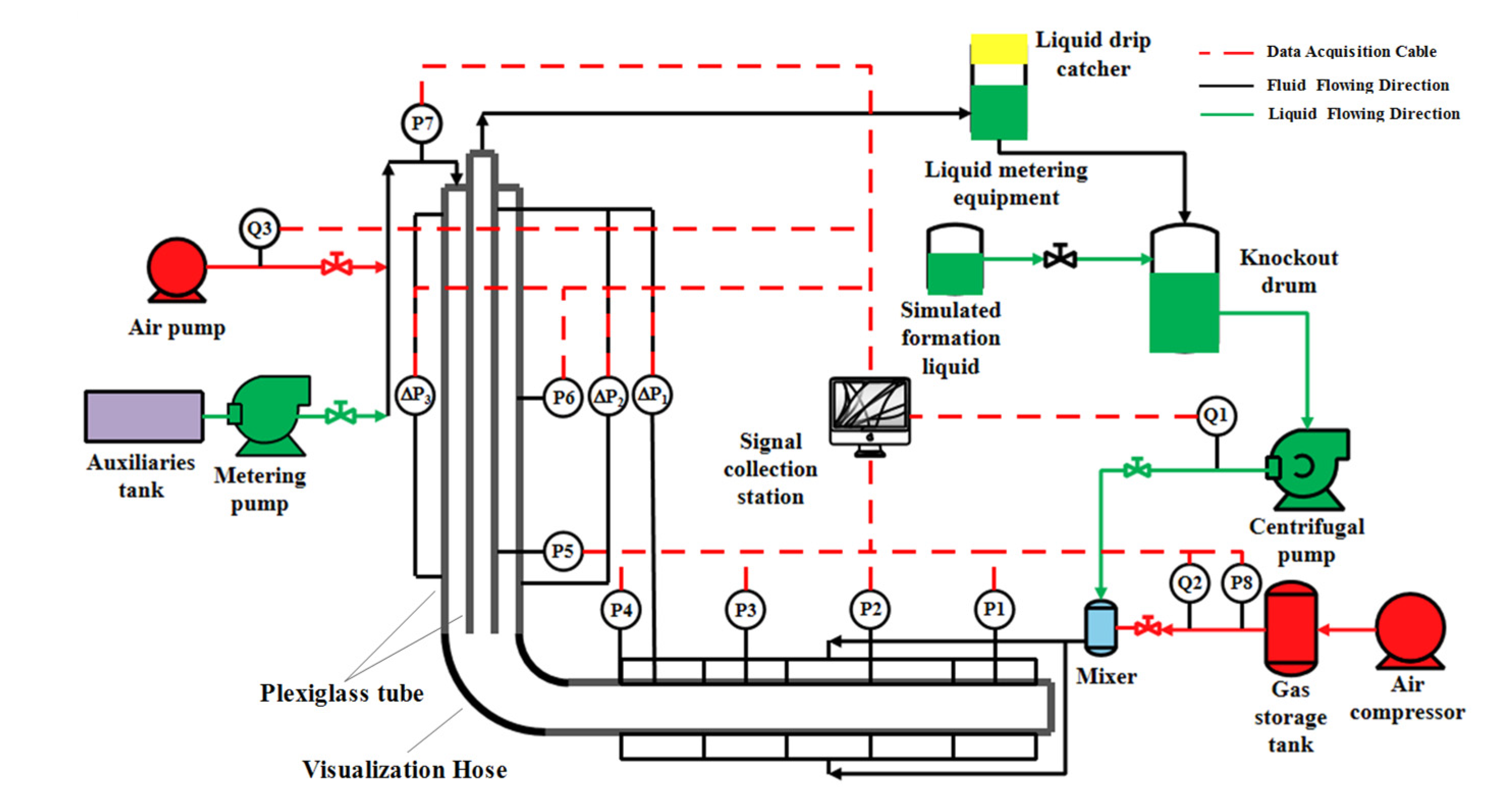
2.3. Experimental Setup

In order to compare and analyze the liquid-carrying capacity of gas flow in various sections of the horizontal gas well, as well as to study the gas–liquid phase flow law of the horizontal gas well under various tubing depths, the multiphase flow experimental equipment that was already in place was redesigned and upgraded. The horizontal gas well simulation device had the precise discharge metering equipment, gas injection equipment, foam addition facilities, etc. Figure 2 displays the schematic representation.

The experimental apparatus is shown in Figure 2 for a horizontal gas well, a circulating water supply system, a gas supply system, and a data monitoring and acquisition system. The high-speed camera, temperature sensor, data acquisition component, computer, and a set of 11 pressure monitoring points, 2 temperature monitoring points, and 4 flow monitoring points make up the acquisition and monitoring system. The casing inner diameter is 60 mm, and the tubing has an inner diameter of 30 mm. The length of vertical section is 12.5 m, the inclined section has a complete curvature 3.21 m long. The length of the horizontal section is 12.5 m, of which the simulating type is the shot hole completion when it contacts the reservoir.

The experimental apparatus can continuously record and monitor pressure, differential pressure data, temperature, gas flow, and liquid flow fluctuation law in the pipe of each well section. The wellhead liquid-carrying capacity is used as the experiment’s reference standard, and the pressure monitoring data of different sections are transformed into the pressure gradient using the pipeline’s length at the measuring site. As a steady processing section, the wellhead liquid discharge is compared at 20 s and measured at 0.01 s. The setup offered the opportunity to visually study the dynamic phenomenon of the flowing liquid and drainage process. It could also gather a variety of data for post-analysis, including pressure, temperature, and the rate of liquid-carrying or drainage.

3. Data Analysis

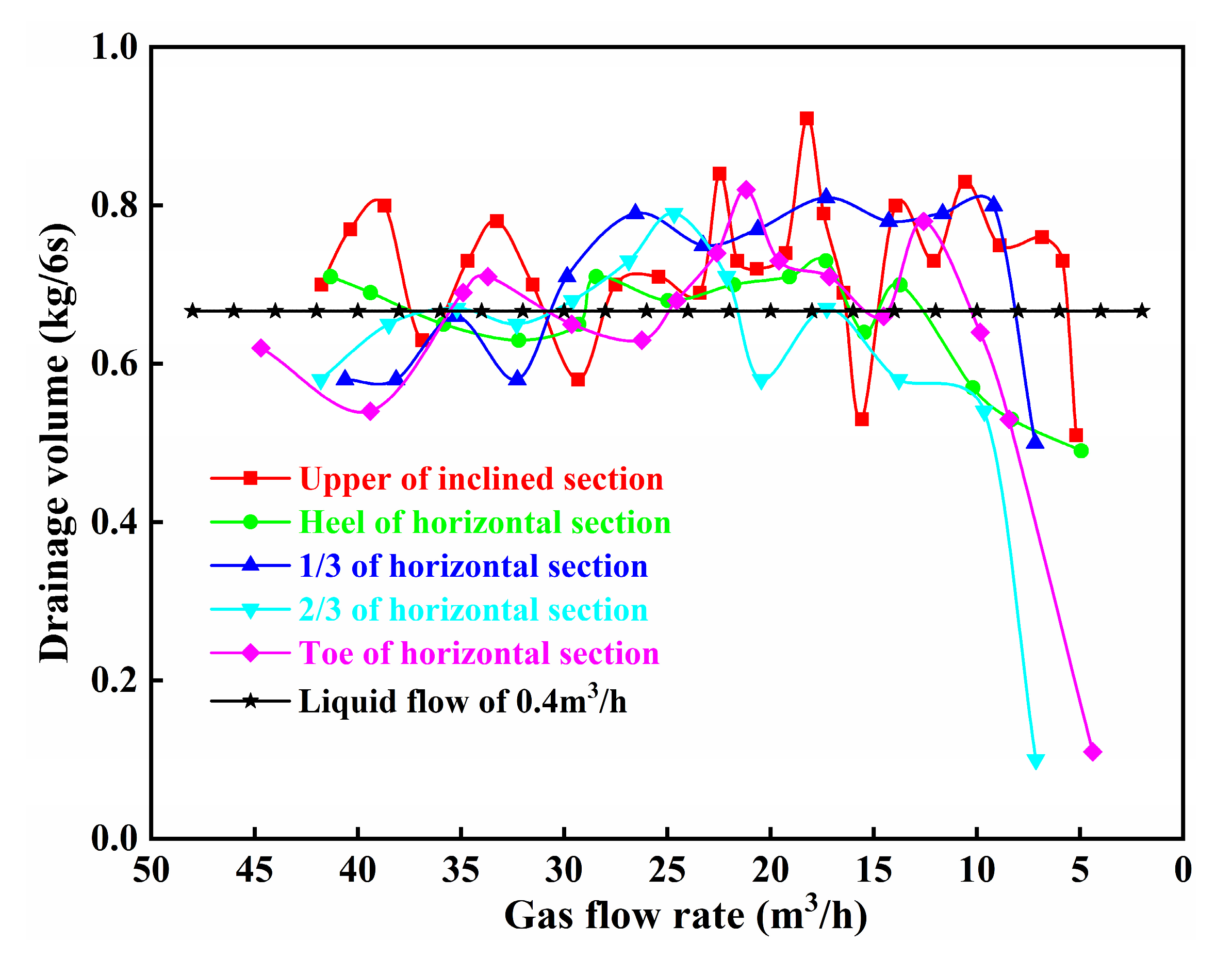
3.1. Drainage Stability

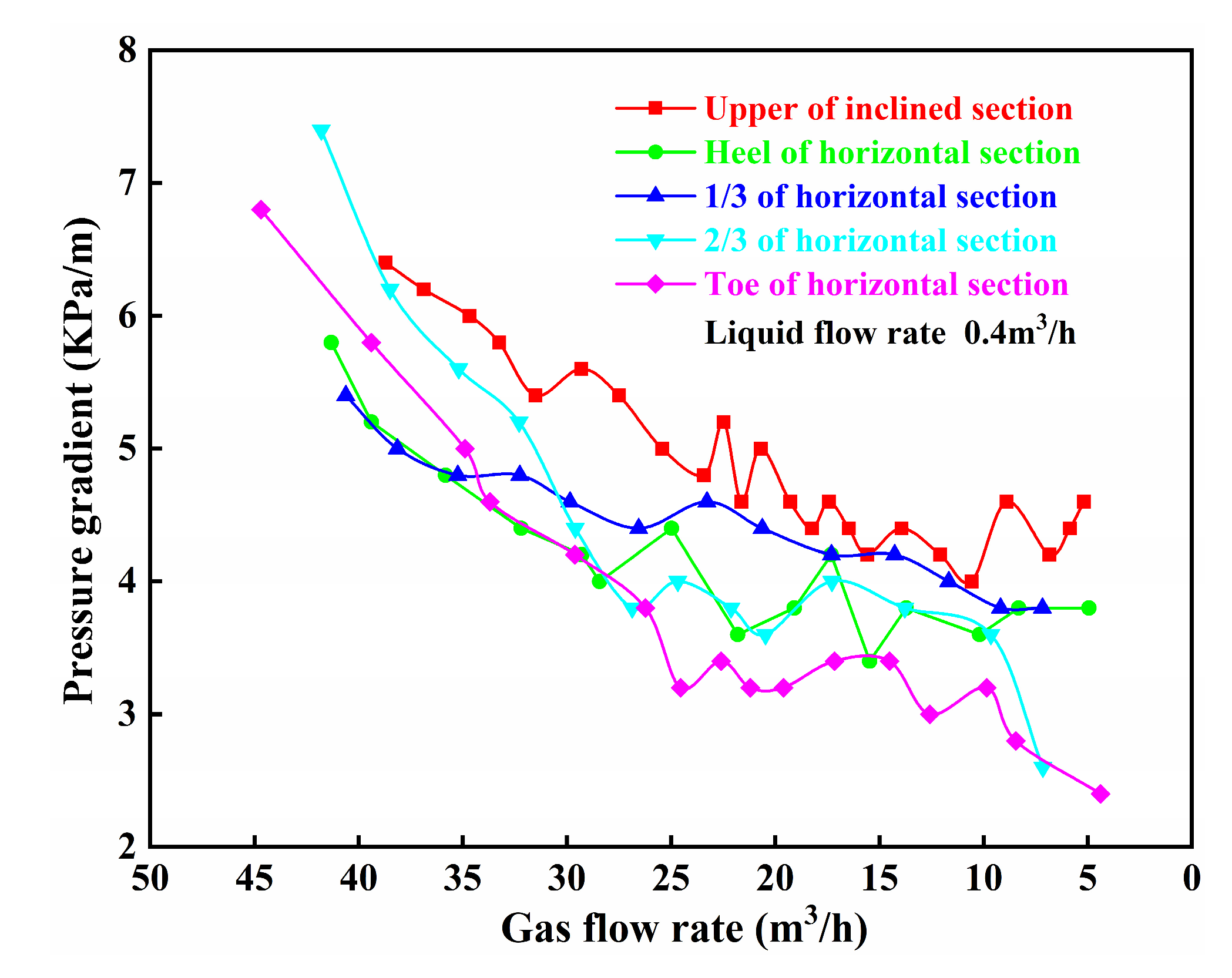
The producing stability of horizontal gas wells has received little attention, although it is crucial to efficient production. Matkivskyi et al., (2021) studied its impact on the ultimate gas recovery and improved the ultimate oil and gas recovery under specific oilfield conditions [53]. Through the use of ordinary pipe, Ma et al., (2022) developed the precision direction by using a full hole method for horizontal gas wells [54]. Bondan et al., (2023) modelled both the downhole and wellhead compressors to see the impact on flow stabilization and wells productivity. They reveal that the downhole compression shows better gain for production rates compared to wellhead compression [55].

The tubing depth defines the diameter distribution of a horizontal gas well and has an impact on the frictional flow resistance. It then has an impact on the liquid-carrying effect. The drainage stability of various tubing depths and the pressure loss of various well sections were first investigated in this article.

Even if the inclined section experiences periodic slug flow due to a progressive decrease in gas flow rate, the liquid can still be continually drained away if the gas flow rate is moderate.

Different tubing depths affect the drainage stability for a specific amount of liquid production rate. Figure 3 illustrates how the drainage volume fluctuates depending on the condition of various tubing depths throughout the flowing process. Figure 3 shows a liquid flow of 0.4 m³/h as an example.

Figure 3 illustrates that the gas well does not load and the generating system can be considered to be in a largely stable state when the gas flow rate is able to remove the liquid. However, the drainage stability varies depending on the tubing depth. As can be seen in

Table 3. Standard deviation between liquid flow rate and production in different tubing depths.

	Liquid Production	0.2 m3/h	0.4 m3/h	0.6 m3/h	0.8 m3/h	1.0 m3/h	1.2 m3/h	1.4 m3/h
Tubing Depth
Upper of Inclined Section		0.09190	0.10327	0.11269	0.13098	0.13624	0.21369	-
Heel of Horizontal Section		0.07991	0.08391	0.08285	0.08407	0.08450	0.08646	0.10624
1/3 of Horizontal Section		0.12320	0.23057	0.16282	0.24958	0.29043	0.21640	0.23225
2/3 of Horizontal Section		0.12997	0.19288	0.24197	0.11533	0.11751	0.35977	0.18563
Toe of Horizontal Section		0.12664	0.18202	0.13269	0.14876	0.20972	-	0.21648

, the fluctuation is typically less when the tubing reaches the heel of the horizontal section than it is in the other sections. It suggests that the wellhead drainage remains more stable with this kind of well structure, which is advantageous to the stability of the systematic production.

The sensitivity analysis of the tubing depth and liquid production rate is displayed in Table 3.

Table 3 demonstrates that the heel of the horizontal section is significantly more advantageous for a stable and continuously producing system. It is suitable for horizontal gas wells with a liquid production range from 5 m³/d to 32 m³/d if the generating liquid can be removed from the wellbore.

3.2. Pressure Loss

The pressure gradient of each section under various liquid flow rates is illustrated in Figure 4, which is based on the two-phase flow laboratory simulation of various tubing depths.

According to Figure 4, each section’s pressure loss is somewhat influenced by the various tubing depths. The pressure loss of the inclined part is almost three times more than that of other sections. By the time the tubing reaches its uppermost point, the horizontal gas well construction resembles the conventional well structure. The flowing direction changes as the fluid moves through the inclined portion as the unique well structure of the inclined section. Gas–liquid two-phase turbulence is created when the fluid is forced to collide with the tubing, severely reducing the gas–liquid two-phase energy. The well tubing starter would also obstruct the fluid’s ability to flow freely through the upper portion of the inclined section. As a result of the drastic shift in flow direction and the increased two-phase slippage, there is an additional energy loss that makes it difficult to remove the liquid from the horizontal gas well. The liquid phase loses more energy than the gas phase.

The pressure loss of the inclined portion is depicted in Figure 5 in accordance with the laboratory simulation, which demonstrates the impact of various tubing depths on this segment’s pressure loss.

At a particular level of liquid output, Figure 5 demonstrates how the pressure in the inclined section gradually drops along with the falling gas flow rate. When the tubing reaches the upper section of the inclined section, the pressure is greater than it is in the previous sections for a given volume of gas and liquid production. Combining the laboratory simulating phenomenon, this might be explained by the fact that the fluid will be seriously impacted by the well tubing starter. When the tubing reaches the upper part of the inclined portion, it would result in significant extra pressure loss in this circumstance.

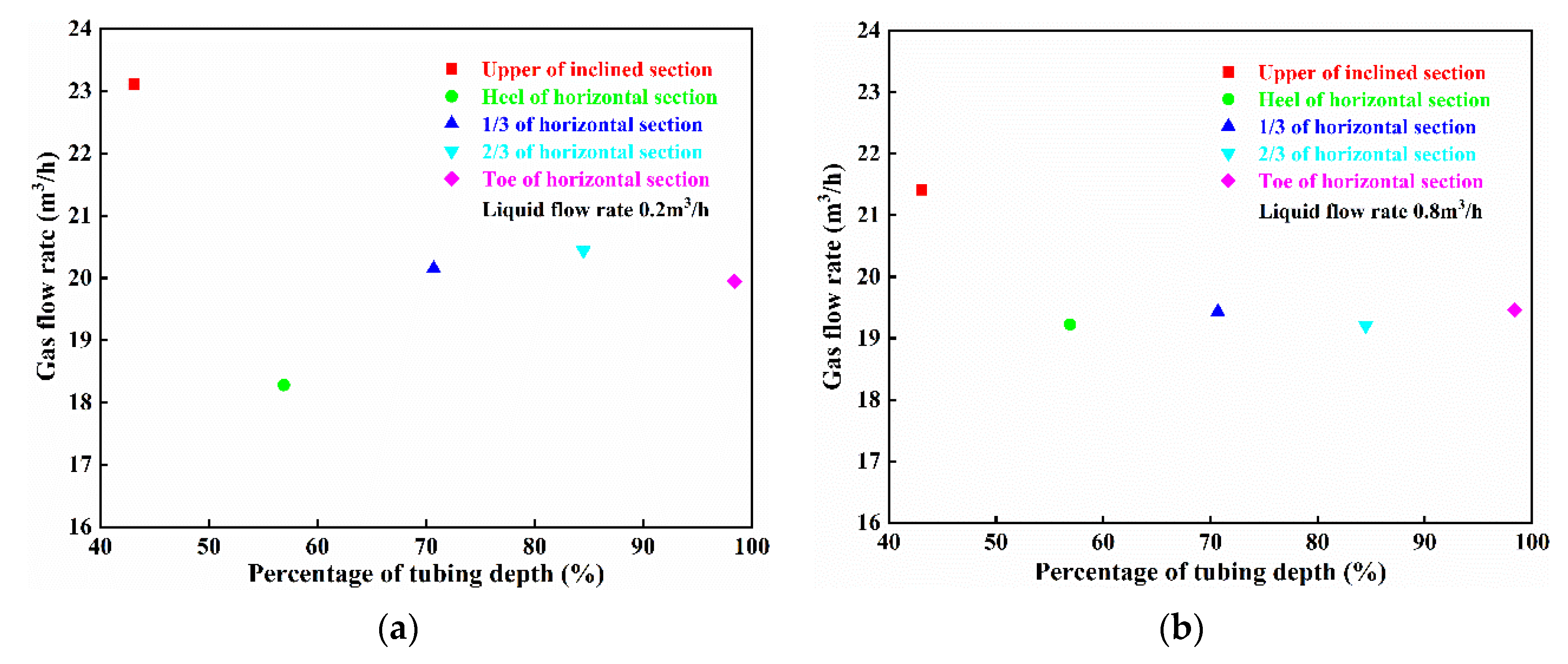
3.3. Liquid-Carrying of Gas Flow Rate

The impact of various tubing depths on the liquid–gas flow rate is depicted in Figure 6. The continuous gas flow rate of the liquid-carrying system is plotted in accordance with varying tubing depths and liquid flow rates.

Figure 6 indicates that if the tubing reaches the heel of the horizontal portion or deeper regions, the gas flow needed for liquid transporting can be relatively little when the produced liquid rate is relatively low. At this point, the sloping segment is the most challenging area for transporting fluids. The tubing diameter of the fluid flow can be effectively lowered when it reaches the heel of the horizontal portion or deeper regions. The gas flow rate in the small-diameter circulation channel is significantly higher under the same gas–liquid flow condition, and the liquid-carrying capacity is improved. As a result, the inclined section is easier for the gas flow to convey the liquid than the other sections. The tubing depth at the heel of the horizontal section can further minimize the gas flow rate necessary for transferring liquid, as shown in Figure 6, given that the produced liquid rate is modest. As a result, the annular gas chamber in the vertical section may have helped the preceding section’s gas drainage during the low liquid rate.

The laboratory simulation results show that tubing depth has a significant impact on the gas drainage and liquid-carrying effect for a conventional well structure. To achieve gas drainage, it reduces the cross-section area of the flow channel, increases the gas velocity, and finally boosts the liquid-carrying capacity. At the same time, it the pipe string discharge technology requires a certain gas flow rate from the gas well. However, taking into account the gas discharge capacity limitation, this method may be appropriate for the low liquid rate of horizontal gas wells.

3.4. Experimental Results

For an accurate estimate of liquid loading, understanding critical gas velocity is important. Theoretically, analytical methods for estimating critical gas velocities can be based on either film or droplet revolution theories, with droplet models being more user-friendly. Although inconsistent across different datasets, droplet model accuracy is not constant. According to prior studies, wellhead pressure and the production ratio affect how accurate droplet models are. Bopbekov et al., (2021) studied the performance of all models against well data in all WHP-GWR categories, as shown in Figure 7 [56].

Liquid loading behavior and critical gas rate prediction are still uncertain. (The new model, as depicted in Figure 7, has a minimum absolute error rate of 16% and is still based on the parameter revised from Bopbekov et al., (2021) [56]). Based on field and experimental data, numerous approaches, correlations, and equations have been put forth to calculate the critical gas velocity and analyze the liquid loading. Nearly all of these analyses suggest the presence of two models (the liquid film model and the droplet model) for the removal of liquid from gas wells. They ignore the energy limit for a specific gas flow rate and rely solely on the force balance of a droplet or a liquid film. The well structure of the horizontal gas well greatly impacts the gas–liquid two-phase flow (shown in Figure 3 and Figure 6), which in turn affects the efficiency of conveying liquid. This causes a large number of research studies on the parameter correction.

Generally speaking, tubing depth has a significant impact on the gas–liquid two-phase flow. The liquid-carrying hypothesis is inappropriate for use in horizontal gas wells, for it ignores the inflow energy of the liquid and gas. This is due to the complexity of the horizontal well structure, the difficulty of effectively accounting for the variables that affect the liquid-carrying capacity, and the complexity of the energy exchange between the gas and liquid phases. As the parameters that affected the liquid-carrying ability are difficult to precisely consider, this paper suggests a novel solution to this issue, arising from the fundamental property of gas–liquid two-phase flow.

4. Model Creation and Laboratory Evaluation

4.1. Model Description and Limitations

Since the structure of horizontal gas wells is more intricate than that of vertical wells, the shape of the liquid-carrying in various sections does not agree well: horizontal gas wells are more difficult to operate. Applying the commonly utilized liquid-carrying hypothesis of vertical gas wells into horizontal gas wells is therefore challenging. The standard theories cannot specify how much liquid can be removed, and they only consider the crucial gas flow rate. In addition, they disregard the fact that the producing liquid has a specific amount of flowing energy, and the gas flow’s capacity to carry liquid is also constrained.

The liquid-carrying capacity of the horizontal gas well is somewhat impacted by the various tubing depths. The inner interaction of the gas–liquid phase may be avoided for the convenience of the analysis. In order to accurately describe the liquid-carrying and quantify the liquid that can be evacuated, the energy of the gas flow and liquid flow should be taken into account. It is necessary to develop a calculating model that accounts for various tubing depths. Only in this way is it possible to accurately quantify the rate of withdrawn liquid and adjust the new theory to account for the actual structure of horizontal gas wells with various tubing depths.

The drainage model of different tubing depths is built in accordance with the laboratory simulation experiment of gas–liquid flow in the horizontal gas well, considering as an example the tubing depth at the top of the inclined section and the heel of the horizontal section. In Figure 8a,b, the physical models are displayed.

Establishing the drainage model and the presumptions used are as follows:

(1)

The volume of liquid withdrawn at the output can be used to roughly calculate the velocity of the discharged liquid at Reference Surface 2.

(2)

The production rates of liquid and gas are constant and continuous at the bottom hole of Reference Surface 1, and the rate should fall within the range of the typical horizontal gas well (as shown in Figure 2 and Table 3).

(3)

During the flowing process, the fluid is only subject to gravity and wall shear stress. No other force is present. The basic characteristics of the producing liquid should be close to the numerical value indicated in Table 2 so that the liquid qualities have little impact on the pipe flow.

(4)

The energy loss produced by the tubing inner wall might be roughly approximated by the local resistance formula.

(5)

The laboratory device’s horizontal section should be straight horizontally or have a tilt angle within ±1 degree.

(6)

As seen in Figure 1 and Figure 2, the horizontal portion of the gas well should be a type of segmented shot hole. It is a tangible representation of the well’s stratigraphic production.

4.2. Model Establishment

The produced liquid enters the horizontal portion, and it appears in the jet condition vertically due to the high liquid density. It can be considered that when fluid enters the horizontal segment, it impacts the tubing vertically.

The liquid is mostly removed from the pipe by the kinetic energy and pressure energy of the gas flow and the liquid flow as a result of output in the horizontal gas wells. After overcoming the effects of gravity, the surface friction of the tubing inner wall, the loss of thermal energy, and the local resistance of the inclined section, the liquid is hoisted to the wellhead. This paper creates a drainage model of various tubing depths using the conservation of energy equation, considering the two reference surfaces presented in Figure 8 for the horizontal gas well as a starting point.

(1) According to the research by Jisheng Y. and Tan X.H. [57,58], the sum of the kinetic energy and the pressure energy of the gas flow can be expressed in per unit time. It can be shown as Equation (6).

$$E_G=\frac{3}{4}{f}_g{\rho }_G{A}_{out1}{v}_G^3+P{B}_g{Q}_G$$

(6)

(2) Similarly, the sum of the kinetic energy and pressure energy of the liquid flow can be expressed in per unit time. It can be shown as Equation (7) [57,58].

$$E_L=\frac{1}{2}{\rho }_{L}g{Q}_L{v}_L^2+P{Q}_L$$

(7)

(3) The gravitational potential energy for a specific amount rate of liquid flow and gas flow necessary to raise the liquid can be stated as Equation (8), which is under the circumstances of a laboratory simulation [59].

$$E_Z=\left({\rho }_{G}g{Q}_G+{\rho }_{L}g{Q}_L\right)h$$

(8)

(4) At various tubing depths, the surface shear stress of the tubing inner wall is active.

The produced gas is subjected to the shear stress of the tubing inner wall when the fluid is hoisted to the wellhead, which depletes the fluid’s kinetic energy.

When the tubing does not reach the end of the horizontal section, namely, $0<{\rm Y}\ll \left(S_v+S_{inc}\right)/\mathrm{S}$, the fluid flows from the heel of the horizontal section to the wellhead. The energy to overcome the shear stress can be shown as Equation (9).

$$E_{F1}={\tau }_{WG1}S{\rm Y}{H}_{gin1}{A}_{in1}+{\tau }_{WG3}\left(1-{\rm Y}\right)S H_{gin2}{A}_{in2}$$

(9)

While the depth of the tubing is deeper than the toe of the horizontal section, namely, $\left(S_v+S_{inc}\right)/\mathrm{S}<{\rm Y}<1$, the fluid flows from the heel of the horizontal section to the wellhead. The energy to overcome the shear stress can be shown as Equation (10).

$$\begin{gathered} E_{F1}={\tau }_{WG1}S{\rm Y}{H}_{gin1}{A}_{in1}+{\tau }_{WG2}\left({\rm Y}-\left(S_v+S_{inc}\right)/S\right)S{H}_{gout1}{A}_{out1} \\ +{\tau }_{WG3}\left(1-{\rm Y}\right)S H_{gin2}{A}_{in2} \end{gathered}$$

(10)

Similarly, when the fluid is lifted to the wellhead, the shear stress of the inner tubing wall acts on the produced fluid, and the fluid kinetic energy is consumed.

When the depth of the tubing does not exceed the heel of the horizontal section, namely, $0<{\rm Y}\ll \left(S_v+S_{inc}\right)/\mathrm{S}$, the liquid flows from the heel of the horizontal section to the wellhead and the inner casing wall works on the liquid produced by the reservoir, which can be expressed as Equation (11).

$$E_{F2}={\tau }_{WL1}S{\rm Y}{H}_{lin1}{A}_{in1}+{\tau }_{WL3}\left(1-{\rm Y}\right)S H_{lin2}{A}_{in2}$$

(11)

While the depth of the tubing is deeper than the end of the horizontal section, namely $\left(S_v+S_{inc}\right)/\mathrm{S}<{\rm Y}<1$, the liquid flows from the end of the horizontal section to the wellhead, and the inner wall of the casing works on the liquid produced by the reservoir. It can be expressed as Equation (12).

$$E_{F2}={\tau }_{WL1}S{\rm Y}{H}_{lin1}{A}_{in1}+{\tau }_{WL2}\left({\rm Y}-\left(S_v+S_{inc}\right)/S\right)S{H}_{lout1}{A}_{out1}+{\tau }_{WL3}\left(1-{\rm Y}\right)S H_{lin2}{A}_{in2}$$

(12)

For the various depths of the tubing, the tubing and casing would work together on the fluid in the wellbore. It can be expressed as Equation (13).

$$E_F=E_{F1}+E_{F2}$$

(13)

According to the study by Fore et al., (2000) [25], the calculation of the shear stress of the wall and the gas can be expressed as Equation (14).

$${\tau }_{WG}=f_G\frac{{\mathsf{\rho }}_{\mathrm{G}}{v}_{\mathrm{G}}^2}{2}, {\tau }_{WL}=f_L\frac{{\mathsf{\rho }}_{\mathrm{L}}{v}_{\mathrm{L}}^2}{2}$$

(14)

In this equation, the gas–liquid friction coefficient can be calculated by the Berrasius equation or the Poisson equation [59], shown as Equation (15).

$$f_L=C_{L}R{e}_L^{-n}, f_G=C_{G}R{e}_G^{-m}$$

(15)

For different flow patterns, turbulent flow ($R{e}_L>2000$, $R{e}_G>2000$), $C_L=C_G=0.046$, $n=m=0.2$. For laminar flow, $C_L=C_G=16$, $n=m=1$. The Reynolds number can be expressed as Equation (16).

$$R{e}_{\mathrm{g}}=\frac{{\rho }_{\mathrm{g}}{v}_{\mathrm{g}}{D}_{\mathrm{g}}}{{\mu }_{\mathrm{g}}}, R{e}_G=\frac{{\rho }_{\mathrm{L}}{v}_{\mathrm{L}}{D}_{\mathrm{L}}}{{\mu }_{\mathrm{L}}}$$

(16)

It can be roughly determined that in the steady state of continuous liquid-carrying, the vertical section exhibits cyclonic flow, the inclined section displays the flow pattern of slug and turbulence, and the horizontal section is essentially in the wavy flow pattern, even though the flow patterns of each section are different. This conclusion is supported by the above laboratory simulation experiment and phenomena. Since the values of the gas and liquid’s friction coefficients vary in various excellent sections, segmenting the data is necessary for calculating the gas–liquid shear stress of the pipe wall.

(5) The fluid temperature will fluctuate to some extent throughout the passage of gas and water in horizontal gas wells. It changes from the horizontal part to the wellhead of the vertical section, leading to a certain energy loss [57]. The specific equation can be expressed as Equations (17) and (18):

The equation for calculating the heat loss of gas is:

$$E_{QG}=C_G{m}_G\left(t_2-t_1\right)=C_G{m}_G∆t$$

(17)

The equation for calculating the heat loss of liquid is:

$$E_{QL}=C_L{m}_L\left(t_2-t_1\right)=C_L{m}_L∆t$$

(18)

(6) In contrast to vertical wells, horizontal gas wells have a unique well structure that includes inclined well sections. The existence of the inclined well section produces an abrupt change in the fluid flow route that damages the liquid flow’s internal structure. Once the vortex and local resistance are created, the liquid flow then needs to reorganize its general structure to account for the new circumstances [57], generating additional local resistance or energy loss. This energy loss can be calculated by referring to the local resistance, which is commonly used on the tubing [60,61]. The specific equation can be expressed as Equations (19) and (20):

$$\mathsf{∆}P=\xi \frac{G^2}{2A_{out1}^2{\rho }_L}\left\{1+\left(\frac{{\rho }_L}{{\rho }_G}-1\right)\left[\frac{2}{\xi }X\left(1-X\right)\mathsf{\Delta }\left(\frac{1}{S}\right)+X\right]\right\}$$

(19)

$$E_S=\xi \frac{v_L^2}{\mathrm{g}}{\rho }_L{Q}_{L1}+\xi \frac{v_G^2}{\mathrm{g}}{\rho }_G{Q}_{G1}$$

(20)

For sliding increments, reference can be made to the laboratory research conclusions of Chisholm et al. [61,62], which can be calculated using empirical Equation (21).

$$\mathsf{\Delta }\left(\frac{1}{S}\right)=\frac{3.7}{2.5+\raisebox{1ex}{$R$}\!\left/ \!\raisebox{-1ex}{$D$}\right.}$$

(21)

Since the value of $R/D$ in different cases is different from that of Chisholm et al., it is necessary to correct the $\xi$ in combination with the laboratory simulation experiment. According to the pressure recording condition of the inclined horizontal section, combined with the calculation method of the shear stress of the fluid on the pipe wall, the local resistance coefficient $\xi$ can be solved under the condition of a certain production liquid gas. The local resistance loss $E_S$ occurs when the gas–liquid two phases pass through the inclined well section [1,26].

(7) When the fluid flows into the horizontal section, there is also local resistance. However, due to the convective state when the fluid flows into the horizontal section [62], the local energy loss can be expressed as Equation (22):

$$E_P=1.3\frac{v_L^2}{g}{\rho }_L{Q}_{L1}+1.3\frac{v_G^2}{g}{\rho }_G{Q}_{G1}$$

(22)

(8) During gas–liquid flow, there exists the slippage, pressure drop loss, and gas expansion effort.

Gas volume changes with pressure; the gas expands and functions. The shear stress also affects the gas phase and the liquid phase in the case of the gas–liquid two-phase flow in the wellbore. Overall, however, the task completed in these two circumstances falls within the category of internal work. Energy is transformed into internal energy, potential energy, and kinetic energy of the two phases. Therefore, based on the conservation of energy, the equilibrium equation of the two-phase fluid is established. In the middle, the work performed by these two internal functions cannot be considered.

According to Equations (6)–(22), the fluid velocity is stable at Reference Surface 1 and 2 when the gas–liquid flow is in a state of stability at various tubing depths. The kinetic energy of the horizontal gas and liquid serves as the sole energy source during the fluid flowing process, allowing for the generation of the following statement.

$$E_{G1}+E_{L1}-E_{QG}-E_{QL}-E_Z-E_F-E_S-E_P=E_{G2}+E_{L2}$$

(23)

When the tubing does not exceed the end of the horizontal section, the calculation formula is expressed as Equation (24):

$$\begin{array}{l}\frac{1}{2}{\rho }_{L}g{Q}_{L2}{v}_{L2}^2+P_{wh}{Q}_{L2}\\ \\ \hspace{1em}\hspace{1em}\hspace{1em}\hspace{1em}\hspace{1em}\hspace{1em}\hspace{1em}\hspace{1em}=\frac{3}{4}{A}_{out1}\left(f_{g1}{\rho }_{G1}{v}_{G1}^3-f_{g2}{\rho }_{G2}{v}_{G2}^3\right)+\left(P_{wf}{B}_{gwf}{Q}_{G1}-P_{wh}{B}_{gwh}{Q}_{G2}\right)+\frac{1}{2}{\rho }_{L}g{Q}_{L1}{v}_{L1}^2+P_{wf}{Q}_{L1}\\ \hspace{1em}\hspace{1em}\hspace{1em}\hspace{1em}\hspace{1em}\hspace{1em}\hspace{1em}\hspace{1em}-\left(C_G{m}_G+C_L{m}_L\right)∆t-\left(\left({\tau }_{WG1}{H}_{gin1}+{\tau }_{WL1}{H}_{lin1}\right),S,{\rm Y},A_{in1},+,\left({\tau }_{WG3}{H}_{gin2}+{\tau }_{WL3}{H}_{lin2}\right),\left(1-{\rm Y}\right),S, ,A_{in2}\right)\\ \hspace{1em}\hspace{1em}\hspace{1em}\hspace{1em}\hspace{1em}\hspace{1em}\hspace{1em}\hspace{1em}-\left({\rho }_{G2}g{Q}_{G2}+{\rho }_{L}g{Q}_{L2}\right)h\end{array}$$

(24)

Similarly, the calculation formula can be obtained when the tubing is deeper than the end of the horizontal section. It is necessary to change the $E_F$, which is accomplished by the pipe wall friction of the gas–liquid two phases.

The research can reveal that the various depths of the tubing have an impact on each well’s flow pattern and shear stress for the gas wells with specific gas and liquid production. It is possible to determine the work performed by the pipe wall shear stress under various tubing depths using the aforementioned Equation (13). During the production process of horizontal gas wells, the gas entering the wellbore at the horizontal portion is consistent with the gas produced under the conditions of the laboratory simulation, $Q_{G1}=Q_{G2}$. Based on the results of the real test, $E_{QG}$, $E_{QL}$, can be determined. In real-world situations, the geothermal gradient can be used to calculate the temperature difference to determine $∆t$ during the production of the entire wellbore. Since the wellhead discharge volume forms the basis for both ends of the theoretical formula, a trial procedure can be used to calculate the volume of liquid discharged at various tubing depths under specific production fluids.

4.3. Laboratory Validation

The established drainage model of various tubing depths was checked and modified based on the laboratory simulation experiment. Theoretical calculation was used to confirm the theoretically predicted depth of the tubing under specific gas output. Figure 9 depicts the model’s predicted outputs.

Figure 9 and statistical examination of mistakes show that the model’s relative error is minimal. According to the statistics, it is 8.41%, 9.02%, 7.76%, 8.6%, and 9.44%, respectively. It satisfies the engineering accuracy standards. There is some viability to the deep drainage type underneath the tubing. A horizontal gas well with a certain gas production can use the model to calculate the liquid discharge at the wellhead. It can also be used as one of the approaches to assess the accumulation of horizontal gas wells.

5. Conclusions and Recommendations

In order to integrate theoretical analysis with laboratory testing to examine the gas–liquid flow law of drainage stability at different tubing depths, we confirmed the impact of gas drainage stability through the lab experiments. This is the foundation upon which a smartly constructed and tested innovative model of varied tubing depths is created. The new model may measure and estimate the amount of liquid pulled from the pipe.

The following conclusions were reached during this study:

(1)

At various tubing depths, the inclined section experiences the greatest pressure loss. When the tubing is positioned closer to the upper part of an inclined section, the liquid collides with the port as it passes through the producing channel, adding to the pressure loss.

(2)

When the tubing depth reaches the end of the horizontal section, the annular gas chamber is frequently compressed and expanded due to the liquid plug sealing effect. It can help with the gas flow discharge. The effect of the sleeve pressure is cyclical when the tubing is lowered to different depths. However, this auxiliary drainage will not take place for the wellhead pressure of the annulus, and will not fluctuate periodically. When it reaches the heel of the horizontal segment, the production system is the most stable.

(3)

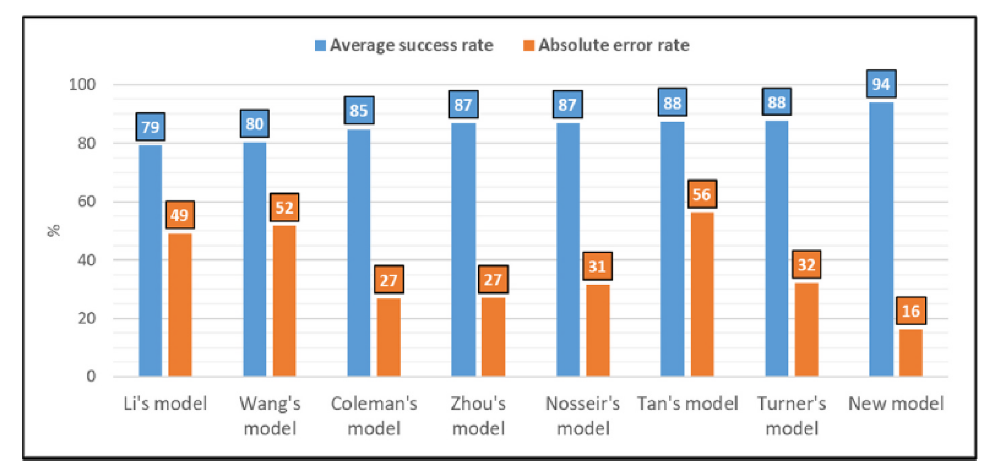
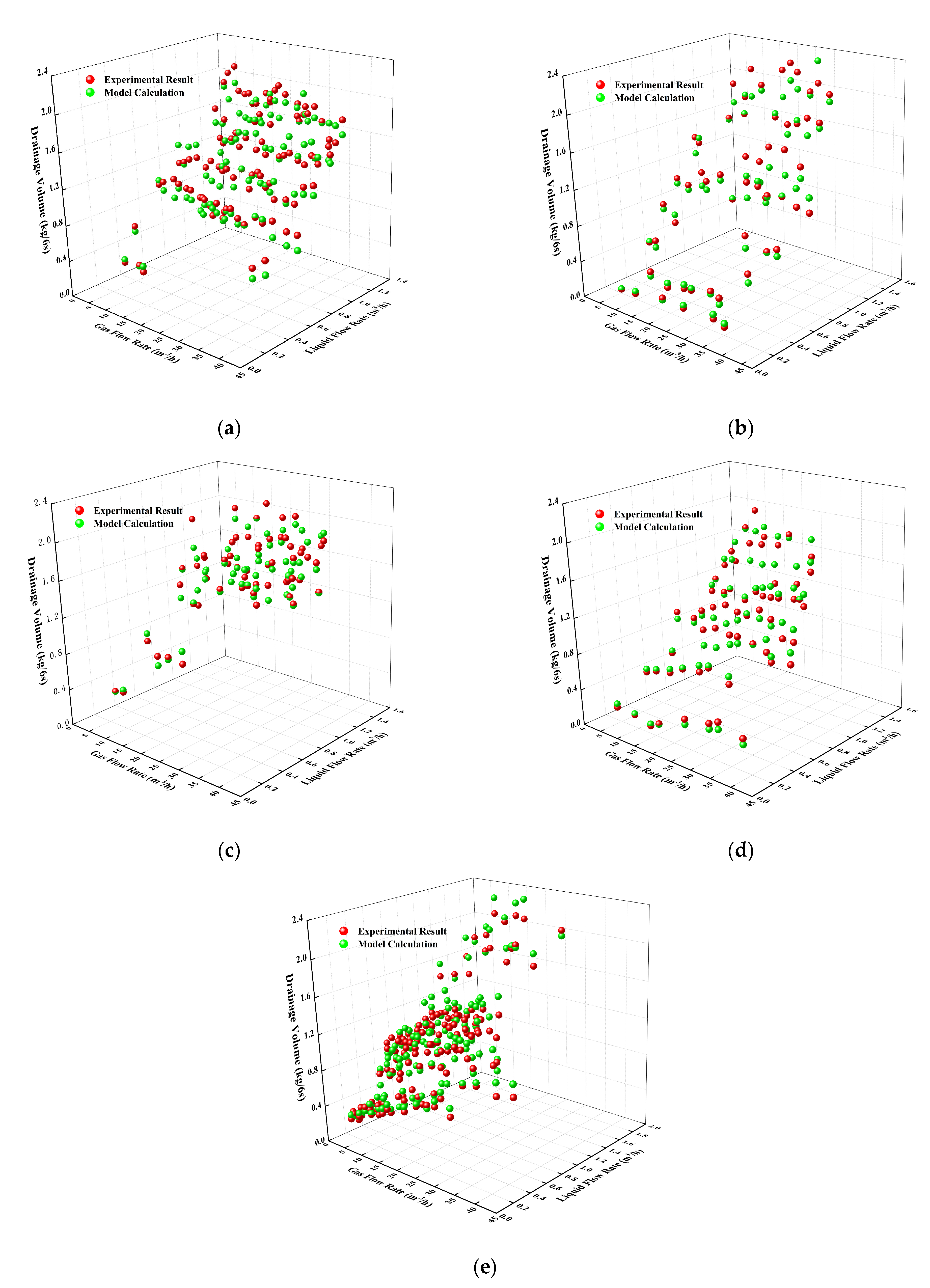
The established new model of various tubing depths is proven using experimental data. The verification outcomes demonstrate the model’s high precision and its applicability as a fresh approach for evaluating the effusion of various tubing depths.

Although the authors performed a thorough examination of pipe flow and developed a useful model for various tubing depths in the horizontal gas well, only laboratory tests were used to validate it. Some elements, such as fluid characteristics, pipe materials, coupling analysis of the influencing factors, and practical application effects, would need to be thoroughly examined in the near future in order to be applied in practice.

References

1. Shekhar, S.; Kelkar, M.; Hearn, W.J.; Hain, L.L. Improved Prediction of Liquid Loading in Gas Wells. SPE Prod. Oper. 2017, 32, 539–550. [Google Scholar] [CrossRef]
2. Joseph, A.; Hicks, P.D. Modelling Mist Flow for Investigating Liquid Loading in Gas Wells. J. Pet. Sci. Eng. 2018, 170, 476–484. [Google Scholar] [CrossRef]
3. Zhang, X. Simulation Experiment of New Drainage Gas Recovery Technology in Horizontal Gas Wells. Master’s Thesis, Southwest Petroleum University, Chengdu, China, 2018; pp. 35–38. [Google Scholar]
4. Wang, Q. Experimental Study on Gas-Liquid Flowing in the Wellbore of Horizontal Well. Ph.D. Thesis, Southwest Petroleum University, Chengdu, China, 2014; pp. 27–29. [Google Scholar]
5. Liu, Y.; Ai, X.; Luo, C.; Liu, F.; Wu, P. A New Model for Predicting Critical Liquid Loading in Horizontal Wells. J. Shenzhen Univ. Sci. Technol. Ed. 2018, 35, 551–557. [Google Scholar]
6. Luan, G.; He, S. A New Model for the Accurate Prediction of Liquid Loading in Low-Pressure Gas Wells. J. Can. Pet. Technol. 2012, 51, 493–498. [Google Scholar] [CrossRef]
7. Turner, R.; Hubbard, M.; Dukler, A. Analysis and Prediction of Minimum Flow Rate for the Continuous Removal of Liquids from Gas Wells. J. Pet. Technol. 1969, 21, 1475–1482. [Google Scholar] [CrossRef]
8. Coleman, S.B.; Clay, H.B.; McCurdy, D.G.; Norris, L.H., III. A New Look at Predicting Gas-Well Load-Up. J. Pet. Technol. 1991, 43, 329–333. [Google Scholar] [CrossRef]
9. Nosseir, M.A.; Darwich, T.A.; Sayyouh, M.H.; El Sallaly, M. A New Approach for Accurate Prediction of Loading in Gas Wells under Different Flowing Conditions. In Proceedings of the SPE Production Operations Symposium, Oklahoma City, OK, USA, 9 March 1997; pp. 241–246. [Google Scholar]
10. Li, J.; Almudairis, F.; Zhang, H. Prediction of Critical Gas Velocity of Liquid Unloading for Entire Well Deviation. J. Pet. Technol. 2015, 67, 97–98. [Google Scholar] [CrossRef]
11. Li, M.; Li, S.L.; Sun, L.T. New View on Continuous-Removal Liquids From Gas Wells. SPE Prod. Facil. 2002, 17, 42–46. [Google Scholar] [CrossRef]
12. Guo, B.; Ghalambor, A.; Xu, C. A Systematic Approach to Predicting Liquid Loading in Gas Wells. SPE Prod. Oper. 2006, 21, 81–88. [Google Scholar] [CrossRef]
13. Belfroid, S.P.C.; Schiferli, W.; Alberts, G.J.N.; Veeken, C.A.; Biezen, E. Prediction Onset and Dynamic Behaviour of Liquid Loading Gas Wells. In Proceedings of the SPE Annual Technical Conference and Exhibition, Society of Petroleum Engineers (SPE), Denver, CO, USA, 21–24 September 2008; pp. 1528–1536. [Google Scholar] [CrossRef]
14. Veeken, K.; Hu, B.; Schiferli, W. Gas Well Liquid-Loading-Field-Data Analysis and Multiphase-Flow Modeling. SPE Prod. Oper. 2010, 25, 275–284. [Google Scholar] [CrossRef]
15. Fiedler, S.; Auracher, H. Experimental and Theoretical Investigation of Reflux Condensation in an Inclined Small Diameter Tube. Int. J. Heat Mass Transf. 2004, 47, 4031–4043. [Google Scholar] [CrossRef]
16. Zhang, L.H.; Luo, C.C.; Liu, Y.H.; Zhao, Y.L.; Xie, C.Y.; Xie, C. A Simple and Robust Model for Prediction of Liquid-Loading Onset in Gas Wells. Int. J. Oil Gas Coal Technol. 2021, 26, 245–262. [Google Scholar] [CrossRef]
17. Zhao, H.; Nguyen, D.; Edgington-Mitchell, D.; Soria, J.; Liu, H.-F.; Honnery, D. The Largest Diameter of Falling Drop in the Up-Gas Flow. Int. J. Multiph. Flow 2022, 159, 1–5. [Google Scholar] [CrossRef]
18. Zang, D.Z.; Wang, Z.B.; Yu, Z.G.; Zhang, R.J.; Yang, B. Calculation Method of Critical Liquid-Carrying Flow Rate of High Liquid-Gas Ratio Gas Well. Fault-Block Oil Gas Field 2022, 29, 411–416. [Google Scholar]
19. Wang, X.; Lu, G.; Luo, C.C.; Liu, Y.H. Method for Calculating Critical Liquid Carrying Flow Rate of Oil-Gas-Water Three-Phase Horizontal Wells. J. Southwest Pet. Univ. (Sci. Technol. Ed.) 2022, 44, 167–175. [Google Scholar]
20. Shan, L.; Song, Y.; Zhou, S.; Liang, G. Experimental and Numerical Study of Droplet Impact on Radially Flowing Liquid Film. Ind. Eng. Chem. Res. 2023, 62, 2008–2020. [Google Scholar] [CrossRef]
21. Duke-Walker, V.; Musick, B.J.; McFarland, J.A. Experiments on the Breakup and Evaporation of Small Droplets at High Weber Number. Int. J. Multiph. Flow 2023, 161, 1–16. [Google Scholar] [CrossRef]
22. Zabaras, G.; Dukler, A.E.; Moalem-Maron, D. Vertical Upward Co-current Gas-Liquid Annular Flow. AIChE J. 1986, 32, 829–843. [Google Scholar] [CrossRef]
23. Barnea, D. Transition from Annular Flow and From Dispersed Bubble Flow—Unified Models for the Whole Range of Pipe Inclinations. Int. J. Multiph. Flow 1986, 12, 733–744. [Google Scholar] [CrossRef]
24. Luo, S.; Kelkar, M.; Pereyra, E.; Sarica, C. A New Comprehensive Model for Predicting Liquid Loading in Gas Wells. SPE Prod. Oper. 2014, 29, 337–349. [Google Scholar] [CrossRef]
25. Fore, L.; Beus, S.; Bauer, R. Interfacial Friction in Gas–Liquid Annular Flow: Analogies to Full and Transition Roughness. Int. J. Multiph. Flow 2000, 26, 1755–1769. [Google Scholar] [CrossRef] [Green Version]
26. Wallis, G.B. One-Dimensional Two-Phase Flow; McGraw-Hill: New York, NY, USA, 1969. [Google Scholar]
27. Pagou, A.L.; Han, G.; Peng, L.; Dehdah, O.; Kamdem, V.G.; Abimbola, F.; Mccarthy, S.A.; Tchomche, H.F.; Harmash, I.; Kanturina, Z. Liquid Loading Prediction and Identification Model for Vertical and Inclined Gas Wells. J. Nat. Gas Sci. Eng. 2021, 84, 1–12. [Google Scholar] [CrossRef]
28. Ke, W.; Hou, L.; Wang, L.; Niu, J.; Xu, J. Research on Critical Liquid-Carrying Model in Wellbore and Laboratory Experimental Verification. Processes 2021, 9, 923. [Google Scholar] [CrossRef]
29. Wang, L.-S.; Liu, S.; Hou, L.-T.; Yang, M.; Zhang, J.; Xu, J.-Y. Prediction of the Liquid Film Reversal of Annular Flow in Vertical and Inclined Pipes. Int. J. Multiph. Flow 2021, 146, 1–25. [Google Scholar] [CrossRef]
30. Dou, N.H.; Ke, K.; Bao, H.Z.; Fu, W.Q. A New Method to Predict Liquid Loading in Wellbore Based on Critical Velocity of Film Generation. China Offshore Oil Gas 2022, 34, 141–146. [Google Scholar]
31. Li, J.C.; Deng, D.M.; Shen, W.W.; Chu, L.P.; Gao, Z.Y.; Gong, J. A New Prediction Model of the Critical Gas Velocity for Liquid Loading in Deviated Gas Wells. Acta Pet. Sin. 2022, 43, 708–718. [Google Scholar]
32. Liu, J.; Jiang, L.; Ye, C.; Cai, D.; Li, J.; Liu, Z.; Yuan, H. A New Calculation Model of Critical Liquid-Carrying Velocity in Inclined Wells Based on the Principle of Liquid Film Delamination Slippage. J. Pet. Sci. Eng. 2022, 216, 1–14. [Google Scholar] [CrossRef]
33. Ma, R.L.; Ma, T.X.; Kang, J.Y.; Yang, K.; Li, L.S.; Wang, L. Prediction Model of Critical Liquid-Carrying Gas Velocity for High Gas-to-Liquid Ratio Gathering Pipelines. J. Pipeline Sci. Eng. 2023, 3, 93–100. [Google Scholar] [CrossRef]
34. Vieira, C.; Stanko, M. Applicability of Model for Liquid Loading Prediction in Gas Wells. In Proceedings of the SPE Europec featured at 81st EAGE Conference and Exhibition, London, UK, 3–6 June 2019; pp. 1–14. [Google Scholar]
35. Bissor, E.H.; Yurishchev, A.; Ullmann, A.; Brauner, N. Prediction of the Critical Gas Flow Rate for Avoiding Liquid Accumulation in Natural Gas Pipelines. Int. J. Multiph. Flow 2020, 130, 1–19. [Google Scholar] [CrossRef]
36. Pan, J.; Pu, X.; Wang, W.; Yan, M.; Wang, L. A prediction Model for the Critical Liquid-Carrying Velocity of Gas–Liquid Stratified Flow in Micro-Tilting Line Pipes with Low Liquid Contents. Nat. Gas Ind. B 2020, 7, 380–389. [Google Scholar] [CrossRef]
37. Cai, W.; Huang, Z.; Mo, X.; Zhang, H. Velocity String Drainage Technology for Horizontal Gas Wells in Changbei. Processes 2022, 10, 2640. [Google Scholar] [CrossRef]
38. Han, B.; Gao, Q.; Liu, X.; Ge, B.; Faraj, Y.; Fang, L. Velocity Distribution of Liquid Phase at Gas-Liquid Two-Phase Stratified Flow Based on Particle Image Velocimetry. Flow Meas. Instrum. 2023, 90, 1–19. [Google Scholar] [CrossRef]
39. Yao, T.; Zhang, Y.; Guo, M.; Tuo, Z.; Wang, H.; Zhou, D. Case Study on Diagnosis and Identify the Degree of Bottomhole Liquid Accumulation in Double-Branch Horizontal Wells in PCOC. In Proceedings of the 2021 3rd International Conference on Civil Architecture and Energy Science, Chemical Performance Structure Research and Environmental Pollution Control, E3S Web of Conferences, Hangzhou, China, January 2021; pp. 1–5. [Google Scholar] [CrossRef]
40. Alsanea, M.; Mateus-Rubiano, C.; Karami, H. Liquid Loading in Natural Gas Vertical Wells: A Review and Experimental Study. SPE Prod. Oper. 2022, 37, 554–571. [Google Scholar] [CrossRef]
41. Wright, J.D.; Nakao, S.-I.; Johnson, A.N.; Moldover, M.R. Gas Flow Standards and Their Uncertainty. Metrologia 2022, 60, 1–41. [Google Scholar] [CrossRef]
42. Zhang, H.; Guo, T.; Zhang, Y.; Wang, F.; Fu, C.; Zhu, T.; Huang, B.; Li, Q. Judgment of Horizontal Well Liquid Loading in Fractured Low-Permeability Gas Reservoirs. Pet. Sci. Technol. 2022, 40, 1512–1533. [Google Scholar] [CrossRef]
43. Huang, Z.; Cai, W.; Zhang, H.; Mo, X. Liquid Loading of Horizontal Gas Wells in Changbei Gas Field. Processes 2023, 11, 134. [Google Scholar] [CrossRef]
44. Wang, W.; Zhu, W.; Li, M. Gas—Liquid Flow Behavior in Condensate Gas Wells under Different Development Stages. Energies 2023, 16, 950. [Google Scholar] [CrossRef]
45. Ehinmowo, A.; Adeboye, I.; Aliyu, M. An Improved Model for the Prediction of Liquid Loading in gas Wells using Firefly and Particle Swarm Optimization Algorithms. Niger. J. Technol. Dev. 2022, 18, 258–267. [Google Scholar] [CrossRef]
46. Chen, Y.; Huang, Y.; Miao, B.; Shi, X.; Li, P. Adaptive Anomaly Detection-Based Liquid Loading Prediction in Shale Gas Wells. J. Pet. Sci. Eng. 2022, 214, 1–11. [Google Scholar] [CrossRef]
47. Hong, B.-Y.; Liu, S.-N.; Li, X.-P.; Fan, D.; Ji, S.-P.; Chen, S.-H.; Li, C.-C.; Gong, J. A Liquid Loading Prediction Method of Gas Pipeline Based on Machine Learning. Pet. Sci. 2022, 19, 3004–3015. [Google Scholar] [CrossRef]
48. Ehsan, R.; William, M.N.S.; Ross, E.M.; Christopher, B.P.; Ferdinand, F.H. A Data-Driven Approach to Predict the Critical Gas Flow Rate in Gas Wells. In Proceedings of the SPE Artificial Lift Conference and Exhibition, Galveston, TX, USA, 23–25 August 2022; pp. 1–12. [Google Scholar]
49. Jia, H.; Zhu, J.; Cao, G.; Lu, Y.; Lu, B.; Zhu, H. A Model Ranking Approach for Liquid Loading Onset Predictions. SPE Prod. Oper. 2022, 37, 370–382. [Google Scholar] [CrossRef]
50. Sinchuk, O.; Strzelecki, R.; Sinchuk, I.; Beridze, T.; Fedotov, V.; Baranovskyi, V.; Budnikov, K. Mathematical Model to Assess Energy Consumption Using Water Inflow-Drainage System of Iron-Ore Mines in Terms of a Stochastic Process. Min. Miner. Deposits. 2022, 16, 19–28. [Google Scholar] [CrossRef]
51. Abhulimen, K.E.; Oladipupo, A.D. Modelling of Liquid Loading in Gas Wells Using a Software-Based Approach. J. Pet. Explor. Prod. Technol. 2022, 13, 1–17. [Google Scholar] [CrossRef]
52. Wang, L.-S.; Yang, M.; Hou, L.-T.; Liu, S.; Zhang, J.; Xu, J.-Y. Experimental Investigation of Film Reversal Evolution Characteristics in Gas–Liquid Annular Flow. AIP Adv. 2023, 13, 1–15. [Google Scholar] [CrossRef]
53. Matkivskyi, S.; Kondrat, O. Studying the Influence of the Carbon Dioxide Injection Period Duration on the Gas Recovery Factor During the Gas Condensate Fields Development under Water Drive. Min. Miner. Deposits. 2021, 15, 95–101. [Google Scholar] [CrossRef]
54. Ma, Y.; Xu, W. Research into Technology for Precision Directional Drilling of Gas-Drainage Boreholes. Min. Miner. Depos. 2022, 16, 27–32. [Google Scholar] [CrossRef]
55. Bondan, B.; Mahmoud, M.D.; Alia, B.Z.B.A.S.; Fatima, O.A.; Ihab, N.M.; Mariam, A.H.; Ahmed, M.A.B.; Azer, A.; Allen, R. A Detail Study Evaluating the Impact of Downhole and Wellhead Compression to Optimize Production from Gas Wells with Liquid Loading Issue: An ADNOC Onshore Gas Field Case Study. In Proceedings of the SPE Reservoir Characterization and Simulation Conference and Exhibition, Abu Dhabi, United Arab Emirates, 24–26 January 2023; pp. 1–15. [Google Scholar]
56. Bopbekov, D.; Pourafshary, P.; Hazlett, R. Accuracy of Droplet Models for Liquid Loading Prediction: Analysis of Production Well Parameters. J. Nat. Gas Sci. Eng. 2021, 98, 1–13. [Google Scholar] [CrossRef]
57. Yang, J.; Liu, J. Practical Calculation of Gas Production; Petroleum Industry Press: Beijing, China, 1994. [Google Scholar]
58. Tan, X.-H.; Li, X.-P.; Liu, J.-Y. Model of Continuous Liquid Removal from Gas Wells by Droplet Diameter Estimation. J. Nat. Gas Sci. Eng. 2013, 15, 8–13. [Google Scholar] [CrossRef]
59. Yuan, E. Engineering Fluid Mechanics; Petroleum Industry Press: Beijing, China, 2007. [Google Scholar]
60. Taitel, Y.; Dukler, A.E. A Model for Predicting Flow Regime Transitions in Horizontal and Near Horizontal Gas-Liquid Flow. AIChE J. 1976, 22, 47–55. [Google Scholar] [CrossRef]
61. Shen, H. Experimental Research on the Characteristics of Slug Flow in the Middle of the Elbow. Master’s Thesis, Xi’an Shiyou University, Xi’an, China, 2014; pp. 43–45. [Google Scholar]
62. Guo, L.; Huang, J.; Guo, C. Study of Local Pressure Drop Characteristics of Oil-Gas Two Phase Flow Through Bend. J. Xi’an Jiaotong Univ. 1998, 32, 38–41. [Google Scholar]
Figure 1. Conventional structure of horizontal gas well.
Energies 16 02165 g001
Figure 2. Schematic diagram of experimental device.
Energies 16 02165 g002
Figure 3. Drainage stability of different tubing depth.
Energies 16 02165 g003
Figure 4. Pressure gradient of different sections with different liquid production rate: (a) top of deviated section; (b) heel of horizontal section; (c) 1/3 of horizontal section; (d) 2/3 of horizontal section.
Energies 16 02165 g004
Figure 5. Pressure loss of the deviated section at different depths of tubing.
Energies 16 02165 g005
Figure 6. Gas flow rate of liquid-carrying in different tubing depths: (a) liquid flow rate 0.2 m3/h; (b) liquid flow rate 0.8 m3/h.
Energies 16 02165 g006
Figure 7. Performance of all models against well data in all WHP-GWR categories [56].
Energies 16 02165 g007
Figure 8. Well structure when the tubing reaches the upper part of the inclined section: (a) upper of inclined section; (b) heel of horizontal section.
Energies 16 02165 g008
Figure 9. Comparison of model calculation and experimental result: (a) upper part of the inclined section; (b) heel of the horizontal section; (c) 1/3 of the horizontal section; (d) 2/3 of the horizontal section; (e) toe of the horizontal section.
Energies 16 02165 g009