Application of Machine Learning to Assist a Moisture Durability Tool

Abstract

The design of moisture-durable building enclosures is complicated by the number of materials, exposure conditions, and performance requirements. Hygrothermal simulations are used to assess moisture durability, but these require in-depth knowledge to be properly implemented. Machine learning (ML) offers the opportunity to simplify the design process by eliminating the need to carry out hygrothermal simulations. ML was used to assess the moisture durability of a building enclosure design and simplify the design process. This work used ML to predict the mold index and maximum moisture content of layers in typical residential wall constructions. Results show that ML, within the constraints of the construction, including exposure conditions, does an excellent job in predicting performance compared to hygrothermal simulations with a coefficient of determination, R², over 0.90. Furthermore, the results indicate that the material properties of the vapor barrier and continuous insulation layer are strongly correlated to performance.

1. Introduction

The built environment accounts for almost 40% of global carbon dioxide emissions [1,2]. More than 25% of those emissions, or 11% of total global emissions, is attributed to manufacturing building materials such as steel, cement, plastic, and glass. Between 2013 and 2016, emissions from the built environment were flat. However, after 2016, emissions started to increase again. The emissions growth rate for the past two years was 2% annually in response to increased construction to meet the growing population’s demand. These trends are not sustainable and are certainly not aligned with the goals established in the Paris Agreement, which include a reduction in carbon dioxide emissions of 50% by 2030 [3].

An effort is underway to help architects and engineers reduce energy consumption and carbon emissions associated with the built environment. In the past, the emphasis was on carbon dioxide emissions related to heating, cooling, lighting, and plug loads. However, the amount of carbon dioxide emitted that is associated with the manufacture of building materials is significant. For example, the production of Portland cement alone accounts for almost 8% of global greenhouse gas emissions [4]. As a result, tools and databases are being developed to help architects and engineers carry out life cycle analysis of building materials to minimize carbon dioxide emissions across all segments of the buildings’ value chain. Tools such as EC3 [4], One Click LCA [5], GaBi [6], and the ICE Database [7] are just a few examples of the resources available to provide information regarding the embodied carbon of building materials.

Another example is the use of plastic foam insulation on the exterior of buildings to reduce heating and cooling loads. However, to what extent will the negative impact of the embodied carbon of plastic foam outweigh the energy savings related to the increased insulation value? Addressing this question requires well-characterized material and manufacturing processes to, in part, quantify the embodied carbon. Manufacturers are using international standards to codify this information into what is defined as an Environmental Product Declaration (EPD) [8]. According to the International EPD System, the EPD is an independently verified and registered document that quantifies product life cycle environmental impact in a standardized form that enables a direct comparison [9]. Most importantly, the EPD contains information regarding a material’s embodied carbon that can then be used as part of a life cycle assessment for the building.

This realization has also driven the growth and development of sustainable building materials. In response to environmental regulations such as California’s Buy Clean California Act, manufacturers have begun modifying existing products and developing products with lower global warming potentials [10]. The challenge accompanying these changes is the long-term performance and durability of these materials incorporated in the building envelope. The time to develop and characterize the long-term performance of building materials is certainly not aligned with adopting these new regulations. The iterative process of material development, characterization, and systems testing is complex. The number of elements in residential and commercial wall systems coupled with different environments or climate zones results in tens of thousands of combinations that must be analyzed to evaluate suitability and performance. This process is not only time-consuming but also expensive.

One approach to facilitate material development and deployment in building enclosure systems from the roof to the foundation is machine learning (ML). ML is a subset of artificial intelligence (AI) that can learn by using statistical models and algorithms to recognize patterns in data. This learning is accomplished without an explicit set of instructions or rules.

An extensive literature review has revealed more than 9000 publications that have a connection between advanced data analytics and building performance. Hong et al. focused on 150 publications that applied machine learning to the design, operation, and control of buildings [11]. Machine learning is finding utility in the built environment because it offers several benefits or advantages compared to conventional simulation tools. Speed seems to receive the most attention, provided the data sets are large enough to train the models. Monitoring building performance lends itself to the collection of large data sets. The challenge is what to do with it beyond, for example, temperature control. One case in point is the work by Tzuc et al. They were able to use weather data to train a neural network to model the hygrothermal performance of a vegetative façade [12]. What makes ML attractive when it comes to modeling the performance of systems with large data sets is that there are options. For example, Tijskens and coworkers evaluated or compared three neural networks’ performance to predict a masonry wall’s hygrothermal performance [13]. In this case, they found that a convolutional neural network required less training time and was the best at predicting performance [14]. To facilitate the selection of moisture-durable constructions, Salonvaara and coworkers implemented ML [15]. They demonstrated that an artificial neural network and gradient-boosted decision trees could be used to simulate hygrothermal performance with reasonable accuracy compared to hygrothermal simulations.

Machine learning has been applied to other problems beyond hygrothermal performance. For example, Kim and coworkers applied ML to optimize a double skin façade for performance and aesthetics [16]. In addition, they compared the results to conventional simulations and found that the two were comparable. Another example of an application is predicting the performance of enclosures integrated with phase change materials (PCMs) [17]. In this example, several models were compared to understand the difference in speed and accuracy when selecting suitable PCMs for this application.

ML was also used to optimize the energy performance of buildings [18]. Using design variables similar to those used in EnergyPlus [19], the model determined the optimal design in less than one minute instead of hours using traditional simulation approaches. Furthermore, the deviation between the optimum value obtained using ML and the simulation results using EnergyPlus was less than 3%, indicating good agreement between the two methods.

Bansal et al. [20] used ML to create a metamodel to forecast long-term hygrothermal responses and the moisture performance of light wood frames and massive timber walls. However, the authors note that unless the input data include the full range of variability of the climate variables, the prediction could be inconsistent. That demonstrates the obvious limitation of ML methods: extrapolating outside the ranges of the input variables can but might not necessarily produce erroneous results.

The benefits of ML applied to the built environment are apparent across a wide range of applications. For example, when designing energy-efficient constructions, it is important to account for the hygrothermal performance or the relationship between the movement of heat, air, and moisture through the building envelope and its effect on durability. The two are not mutually exclusive. Depending on the temperature and relative humidity, condensation within the building envelope can occur, resulting in durability problems such as mold and rot. For example, because insulation materials made from natural fibers are inherently a food source, they are more susceptible to mold growth than synthetic materials such as plastic foam insulation. To avoid the issue, hygrothermal simulations are used to evaluate the effect of material properties and wall designs on durability. The approach is complex and requires expert knowledge to implement. However, the benefits of ML can be used not only to facilitate the implementation of new materials in wall construction but also to provide guidance regarding material properties required to achieve a certain level of performance in a wall design. More importantly, such work is possible in the absence of expert knowledge.

The conventional approach to material development and deployment consists of the following steps: (1) new material is developed, (2) hygrothermal properties are characterized, (3) the building envelope material layout is adjusted so the new material can be incorporated, and (4) hygrothermal simulations are carried out to assess performance and durability.

In a wall system, the number and combination of variables that describe its performance are vast, more than tens of thousands when breaking down the levels with respect to material properties and the material layers that make up the wall assemblies. Coupled with climate, the number increases by more than an order of magnitude. Optimizing the materials and systems using an iterative process, as described earlier, requires significant resources, time, and cost.

Another limitation of using hygrothermal simulations is that they can only be carried out in one direction. That is, first, the user determines the properties of the material and then constructs the wall assembly and runs the simulation. Then, the materials and design are refined based on expert knowledge to improve performance. Unfortunately, the simulations cannot be run in the opposite direction where the architect or designer specifies a level of performance and the simulation generates the design or material properties required to meet that level of performance.

Because ML looks at patterns in data sets, it is irrelevant whether the starting point is the material properties or a level of performance at the assembly level. Herein lies the advantage of using ML over conventional simulation methods, and the present paper demonstrates this.

2. Building Science Advisor—New Construction

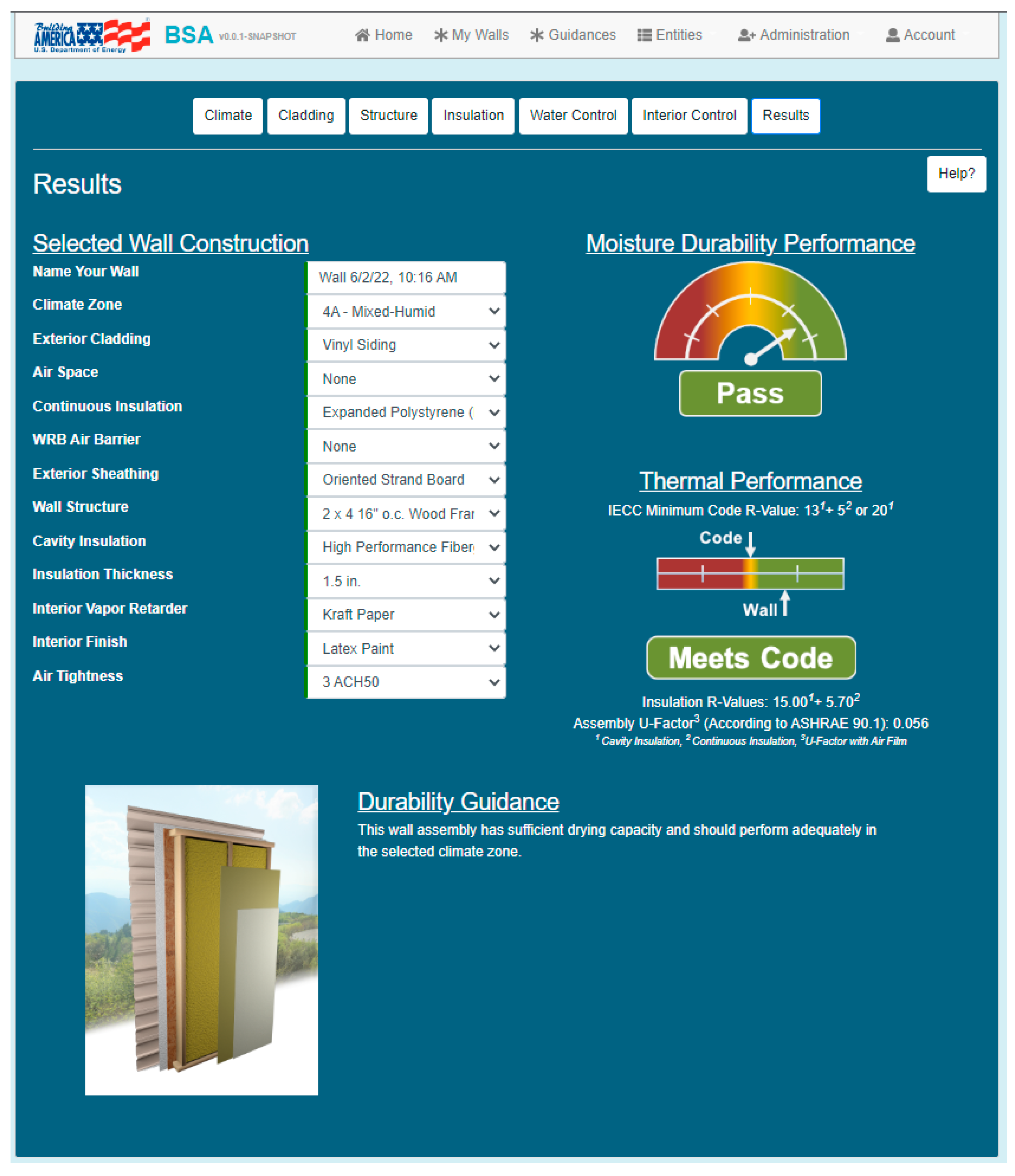
To help architects and engineers select durable enclosure designs with minimal effort, Oak Ridge National Laboratory developed the Building Science Advisor (BSA). The new construction tool guides the user to input the following data for a proposed wall: climate zone, exterior cladding, water-resistive barrier, continuous insulation, sheathing, wall structure type, cavity insulation, and interior vapor barrier. After the user inputs these data, the tool searches a database for similar walls. Each entry into the database includes a set of material properties for some or all the wall layers and an associated moisture durability rating. The moisture durability ratings for the condition described in the entry are pass, inconclusive, or fail. These ratings are based on hygrothermal simulations or expert opinions. The user’s wall can match more than one entry in the database. If this happens, the most conservative durability rating and relevant durability guidance are displayed. The durability guidance will tell the user why the wall did not pass the moisture durability assessment and what can be done to improve the performance of the wall.

Figure 1 shows a presentation of this information for a user-selected wall. The user can see and change the wall construction. The wall’s moisture durability and thermal performance, as well as the wall’s construction visualization and durability guidance, are displayed.

The moisture durability performance is based either on the mold index calculated from the hygrothermal modeling outputs as outlined in ASHRAE Standard 160 or on the consolidated expert opinion [21]. Typically, the entries in the database from hygrothermal simulations specify the material properties of every layer in the wall, and the entries from expert opinion specify only the material properties of select layers. The expert opinion-based entries focus on common issues found in walls that are known to cause long-term moisture durability problems. A more thorough description of how this tool works can be found in the literature [22].

3. Building Science Advisor—Retrofit

The retrofit web tool has similar inputs for the wall construction as the new construction tool. In the retrofit web tool, the user describes the existing wall to be retrofitted and then selects the desired retrofit: exterior, gut, or interior retrofit. Figure 2 shows the materials in the wall that can be changed depending on the chosen retrofit approach. After the user selects the preferred retrofit approach, the tool searches a database of hygrothermal simulation results for matches on the unchanged materials. For example, suppose the user selected an exterior retrofit. In that case, entries in the database are found with the same wall structure, interior vapor retarder, and interior finish as the existing wall.

All matches with a mold index of less than two are presented to the user. The matches can be filtered for desired materials, and then one wall can be selected to view its moisture and thermal performance, which can be compared with the existing wall. Figure 3 shows the result screen for the tool, where the existing and retrofit wall materials, moisture durability, and thermal performance are compared.

The core of these webtools is in the database used to assess the moisture durability of a user’s wall. Most entries for the retrofit and new construction databases are based on hygrothermal simulation results. However, to cover the wide range of layer and material combinations for walls in each climate zone requires millions of simulations, which is expensive in both simulation computing time and server speed when hosted for the webtool. Furthermore, using a static database does not allow flexibility for the user to input new or custom materials to be evaluated in a wall.

4. Hygrothermal Simulations to Create Inputs for Machine Learning

The BSA tool helps users answer design questions regarding thermal performance and durability. Hygrothermal simulations are time-consuming and require expertise not only in heat and mass transfer but also in setting up numerical models to evaluate the performance and risks of the designs. Furthermore, once the simulations have been carried out for a specific design, the remaining question is whether the solution is optimal and what should be completed to make it perform better. Therefore, a quicker and simpler tool is needed to evaluate and optimize the design.

The number of simulations to create a database to cover all possible design options the user might select can rise to millions of cases. That is because each layer in the wall can have multiple options. For example, the input options for the cladding could be different types of brick, fiber cement siding, vinyl siding, wood siding, and others. The water-resistive barrier can be almost water vapor impermeable, very vapor open, or somewhere in between. Wall assemblies with just three options for a 7-layer wall assembly in 15 climates result in more than 30,000 simulation cases in just 1 orientation. Adding options to select would increase the number of cases exponentially.

A standard or typical database includes climate zone, wall orientation, the identity of the layers (e.g., “brick” or “mineral fiber insulation”), description or property of the layers (e.g., “thickness” or “vapor permeability”), and performance parameters (e.g., “mold index” or “maximum moisture content”). Named inputs, or categories, are sufficient in a database that is used only to select the performance for the cases the database includes. In a previous paper, the authors used machine learning to predict performance using categorical inputs [15]. However, when using categorical inputs, the user would not be able to evaluate the performance of a wall with a material layer that is not included in the original data set. Furthermore, interpolating between the simulated cases in the database would not be possible with categorical or named inputs. Therefore, we elected to use the material properties of the layers in the database instead of names or categories of materials, which is what is performed in BSA. These inputs would then be analyzed with ML techniques to interpolate new results between the simulated cases.

Even though the simulations for the BSA tool include mass walls, this paper focuses on lightweight wood frame construction.

4.1. Design Process

Hygrothermal simulations are post-processed per ASHRAE Standard 160 [21] to consider the maximum acceptable moisture content in a critical layer and the mold growth index in the wall. The exterior sheathing was selected as the critical layer. The mold growth index (MI) was calculated on both the exterior and interior sides of the insulated cavity to account for performance in cold and hot-humid climates. Mold growth in the building assembly was predicted by running a five-year simulation and taking the maximum MI. The MI can range from between 0 and 6 [23].

An additional criterion for some materials, such as wood-based sheathing boards, is typically the limit for moisture content. Wood begins to suffer damage if its moisture content remains at 20% for days or longer. High moisture content for a prolonged period can allow the wood to begin to rot. In addition, dimensional changes due to high moisture can further create damage and impact the integrity of the building envelope assembly.

4.2. Wall Assemblies and Climates Included in the Study

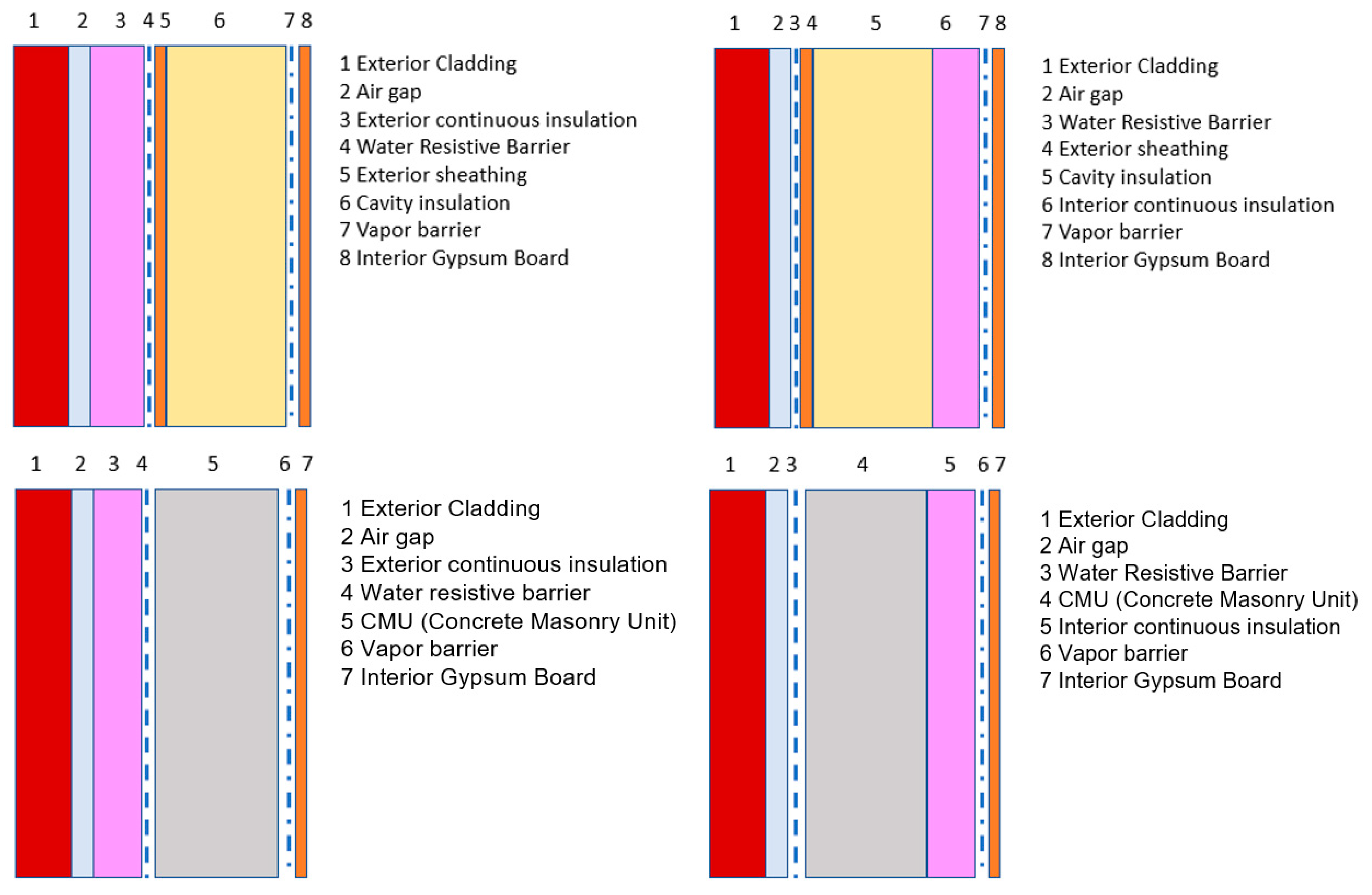
One-dimensional simulations were carried out for lightweight and masonry walls using a hygrothermal simulation tool [24]. The simulation parameters used in the training set included 19 climate locations covering all 8 US climate zones and the wall structures, as depicted in Figure 4. The simulations included the locations and climate zones listed in

Table 1. Locations and climate zones used in simulations for hygrothermal performance. Italicized locations were used as testing climates and were not part of the training set for ML.

Location	Climate Zone	Climate Characteristic
Miami, FL	1A	Hot humid
Houston, TX	2A	Hot humid
Mobile, AL	2A	Hot humid
Phoenix, AZ	2B	Hot dry
Tucson, AZ	2B	Hot dry
Atlanta, GA	3A	Mixed humid
Los Angeles, CA	3B	Hot dry
San Francisco, CA	3C	Marine
Baltimore, MD	4A	Mixed humid
Knoxville, TN	4A	Mixed humid
Albuquerque, NM	4B	Mixed dry
Seattle, WA	4C	Marine
Chicago, IL	5A	Cold wet
Madison, WI	5A	Cold wet
Syracuse, NY	5A	Cold wet
Grand Island, NE	5A	Cold wet
Flagstaff, AZ	5B	Cold dry
Minneapolis, MN	6A	Cold wet
Burlington, VT	6A	Cold wet
Boise, ID	6B	Cold dry
Anchorage, AK	7	Very cold
Fairbanks, AK	8	Subarctic

. Mobile, AL, Grand Island, NE, and Burlington, VT, were used to test the model’s ability to predict performance; hence, they were not part of the training set.

The layer details are listed in

Table 2. Layer options for the lightweight and the masonry walls used in parametric simulations, adapted from ref. [15].

Layer	Lightweight Wall	Masonry Wall
Brick, buff matt brick, vinyl, fiber cement, stucco, wood	X
Vinyl, stucco		X
Ventilated, nonventilated air gap	X	X
Continuous insulation, extruded polystyrene (XPS), expanded polystyrene, mineral fiber, cork (0/16/25/38/51/76/102 mm)
Water-resistive barrier, permeance: 0.5, 5, 10, or 50 perms	X	X
OSB (oriented strand board), plywood, chipboard, wood fiberboard, wood, exterior grade gypsum board	X
89 mm or 140 mm wood frame	X
203 mm CMU (concrete masonry unit), grouted or ungrouted		X
Cavity insulation: Fiberglass, closed-cell spray foam, no insulation	X
Interior continuous insulation: None, 25 mm XPS, 25 mm mineral fiber	X
Vapor retarder: None, 0.5/1/5 perm, variable permeance	X	X
Gypsum wallboard and latex paint	X	X

.

4.3. Example of Simulation Results for Machine Learning Analyses

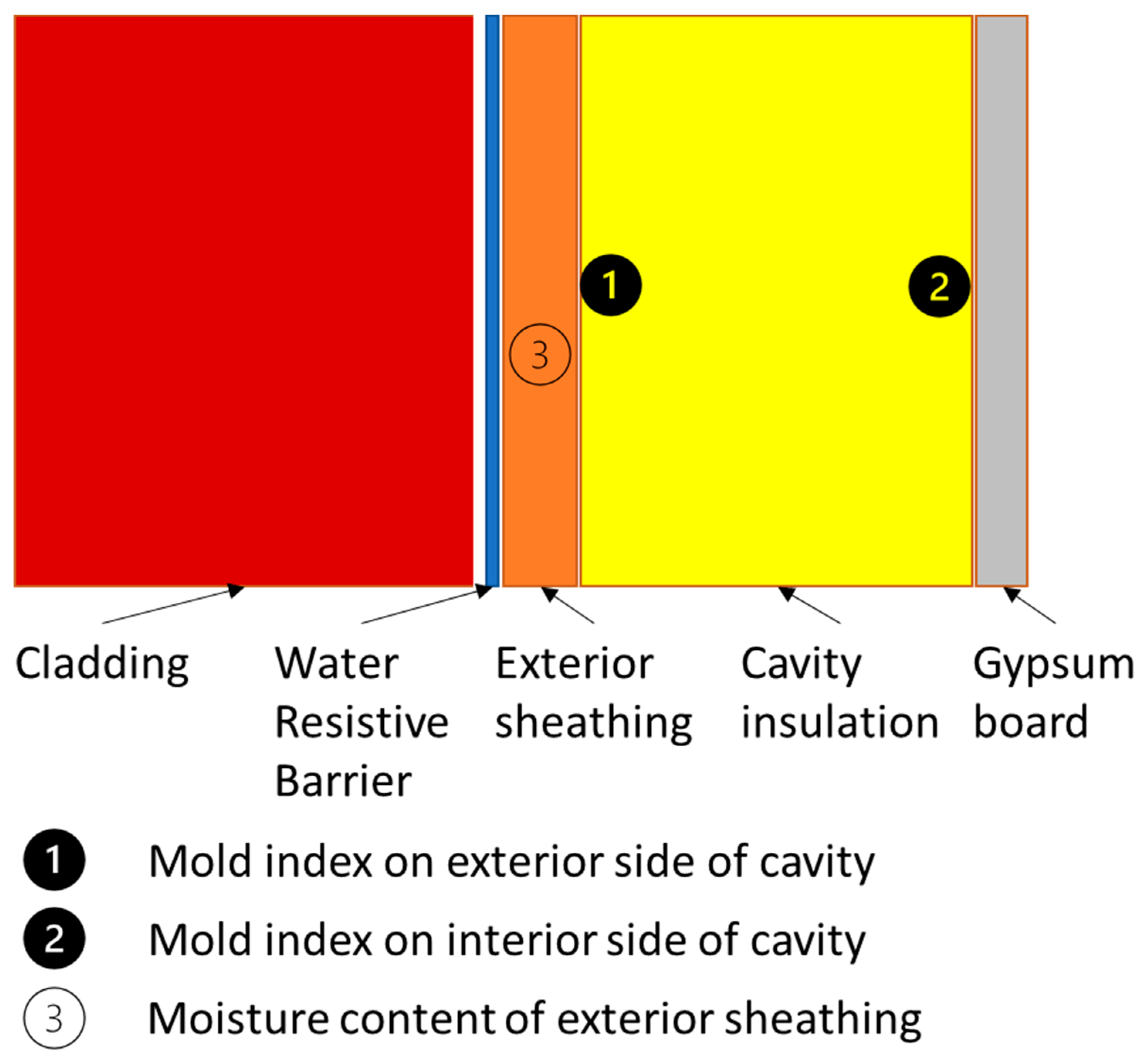
The performance data for ML analyses were created by running hygrothermal simulations for wall assemblies in different climates. An example of a wall system, its layers, and locations of interest are shown in Figure 5. The simulations were run for five years using the same single-year weather file. The moisture design reference year (second most severe year) per the ASHRAE Research Project 1325 [25] was used in each climate location. Three key values are taken from each simulation: (1) temperature and relative humidity on the exterior side of the insulated cavity (Point 1), (2) temperature and relative humidity on the interior side of the cavity (Point 2), and (3) average moisture content of the exterior sheathing (Point 3). The hourly temperature and relative humidity were used in postprocessing to calculate the predicted mold index for Points 1 and 2.

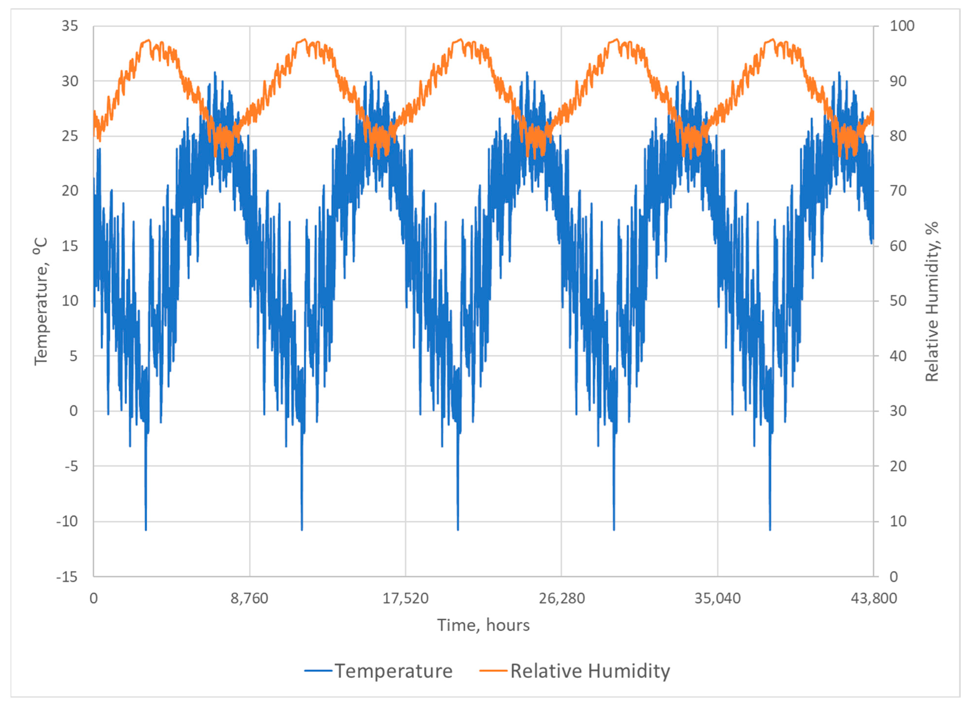
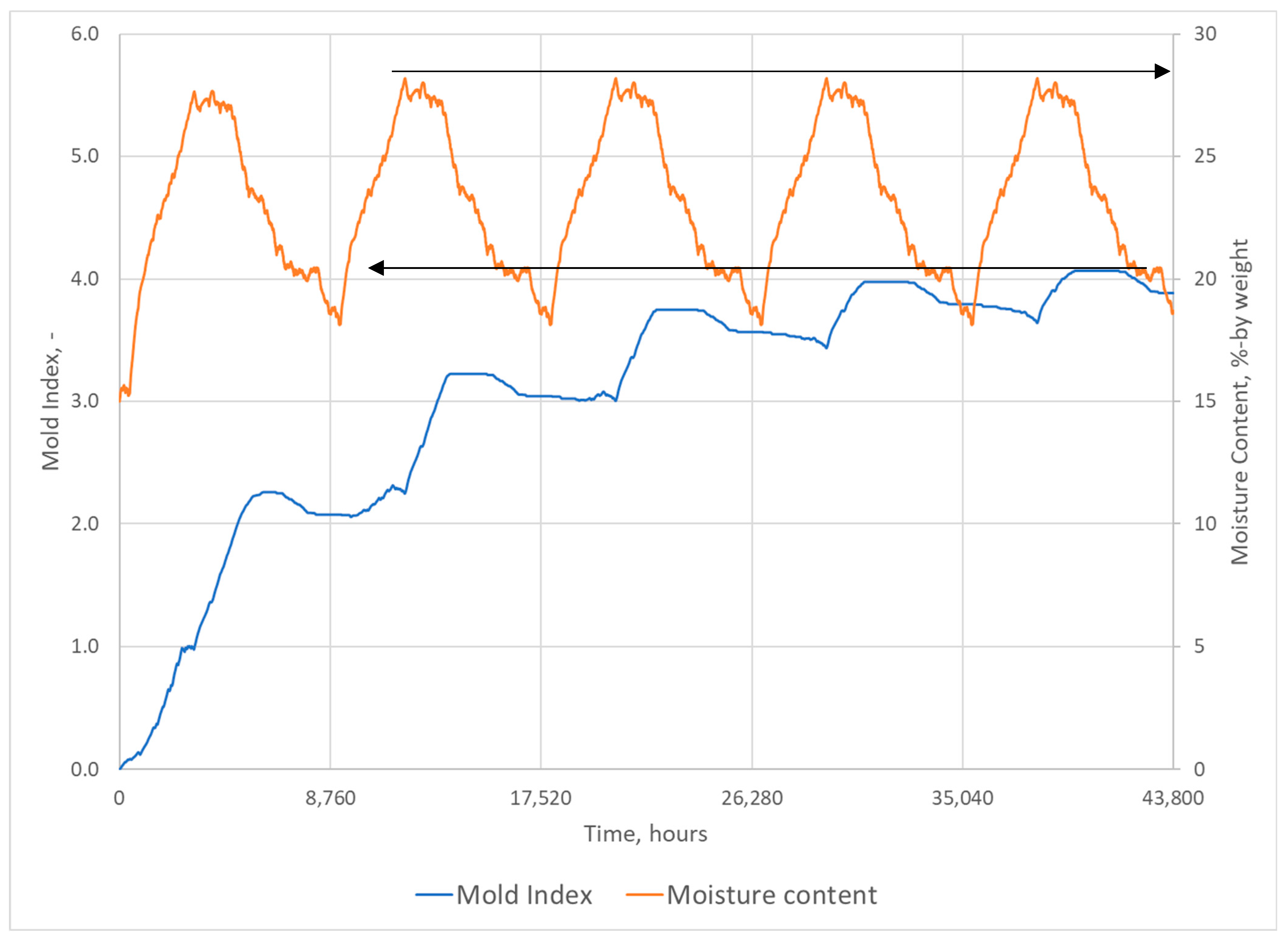
The maximum mold index and moisture content values over the five years were then recorded for each case as the performance value and inputs for ML analyses. Figure 6 shows the hourly temperature and relative humidity on the exterior side of the insulated cavity. Figure 7 shows the post-processed mold index and the average moisture content of the exterior sheathing. The maximum values of the mold index and the moisture content over the simulated period are selected as the final values. The mold index is calculated both for the exterior and the interior side of the insulated wall cavity. The highest mold index of the two is selected as the final performance value.

The data for performance analysis based on the results in Figure 7 would be a mold index slightly above 4 and a maximum moisture content of about 28% by weight.

4.4. Creating Inputs from Simulation Cases for Machine Learning Analysis

This paper focuses on the analysis of wood-framed walls. These cases form 87% of the cases in the database.

Named materials and thicknesses describe a wall in each functional layer of the wall, such as cladding, continuous insulation, and water-resistive barrier. In this study, we converted the named layers in the simulated wall assemblies into numeric values describing each layer with relevant material properties for heat and moisture transport. Using regression analysis with ML, these numeric values allow for a correlation between the performance values and the inputs (material properties and weather parameters).

Cladding materials are exposed to rain and ambient air temperature and humidity. Therefore, the cladding materials were characterized by the liquid uptake value (A-value, kg/m²∙s⁰⁵), water vapor permeance (1 U.S. Perm = 57 ng/s∙Pa ∙m²) for so-called dry-cup and wet-cup conditions (0%RH-50%RH and 50%RH-100%RH, respectively), moisture storage (sorption at 80%RH, W80, kg/m³), and thermal resistance R (m²∙K/W). The exterior sheathing materials were characterized with the same parameters but without the liquid uptake value. The water-resistive barriers (WRBs) and vapor retarders had only the water vapor resistance values for dry- and wet-cup conditions. Instead of giving the permeance values of layers as inputs for the model, we used the water vapor resistance, Z = 1/permeance. Finally, the insulation layers were characterized by the water vapor permeance (given in input as water vapor resistance, Z) and thermal resistance values. The properties of materials used in the simulations are shown in

Table 3. Materials and properties.

Materials	k-Dry (W/m∙K)	A-Value, kg/m2∙s0.5	Permeance, Dry Cup, Perm	Permeance, Wet Cup, Perm	W80, kg/m3	Thickness (m)	R-Value (m2∙K/W)
Exterior sheathing
OSB	0.092		0.62	5.56	83.4	0.0125	0.136
Plywood (USA)	0.084		0.58	8.77	64.4	0.0150	0.179
Southern yellow pine	0.119		0.38	8.33	62.2	0.0200	0.168
Wood fiberboard	0.052		16.67	20.00	35.4	0.0125	0.240
Exterior gypsum	0.218		45.45	58.82	6.2	0.0127	0.058
Claddings
Buff matt clay brick	0.43	0.00013	1.19	4.54	2.4	0.1040	0.242
Brick old	0.4	0.2083	2.56	4.35	3.3	0.1040	0.260
Vinyl siding		0	0.10	0.10	0		0.018
Stucco	0.399	0.0033	1.02	2.08	106.6	0.0200	0.050
Western red cedar	0.084	0.0011	0.21	1.02	33.7	0.0200	0.238
Fiber cement siding	0.245	0.03	2.08	20.00	185.8	0.0080	0.033
Vapor retarders
PA membrane			0.88	16.67
VB: 0.1 perm			0.1	0.10
VR: 0.5 perm			0.5	0.50
VR: 1.0 perm			1	1.00
VR: 5.0 perm			5	5.00
WRBs
WRB: 0.5 perm			0.50	0.50
WRB: 5.0 perm			5.00	5.00
WRB: 10 perm			10.00	10.00
WRB: 50 perm			50.00	50.00
Cavity insulation			Permeance per inch				R-value per inch
Fiberglass			118				0.652
Closed-cell spray foam			1.46				1.057

.

Additionally, to evaluate the performance in a more refined location and weather conditions, the climatic information was converted to annual weather parameters to assess the ability of ML to correlate the hygrothermal performance to the weather parameters. In the ASHRAE Research Project 1325, “Environmental weather loads for hygrothermal analysis and design of buildings,” [25] annual weather parameters were found to correlate with the durability performance of wall assemblies, and the method to select moisture reference years was created using annual average weather parameters. Therefore, it is reasonable to assume that the weather parameters could be used in the ML analyses instead of named weather locations as categorical inputs.

Table 4. Average annual weather parameters for weather locations. Solar radiation and wind-driven rain are shown for two orientations: north (N) and the orientation of the wall that receives most of the wind-driven rain (WDR). The locations in italics were used as testing locations and were not part of the training set.

City, State	T (ºC)	RH (%)	Pv (Pa)	Cloud -	RadN (W/m2)	RadWDR (W/m2)	RainN (mm/h)	RainWDR (mm/h)	Av.Tmin (ºC)	Av.Tmax (ºC)
Miami, FL	24.5	73.3	2031	3.8	70	88	0.0651	0.0799	20.7	28.5
Houston, TX	18.7	78.9	1762	4.2	62	78	0.0651	0.0713	13.4	24.8
Mobile, AL	18.7	74.6	1663	4.2	62	116	0.0734	0.0982	14.2	24.2
Phoenix, AZ	23.3	43.2	1113	2.6	59	116	0.0080	0.0171	17.3	29.4
Tucson, AZ	18.9	37.0	987	2.5	59	158	0.0135	0.0227	12.0	25.9
Atlanta, GA	14.7	71.4	1357	4.4	63	104	0.0386	0.0713	10.1	20.0
Los Angeles, CA	17	75.8	1478	3.6	64	126	0.0070	0.0435	13.7	21.2
San Francisco, CA	13.9	78.0	1261	3.7	56	133	0.0034	0.0775	10.4	18.6
Baltimore, MD	12.4	68.7	1218	4.2	56	70	0.0599	0.0720	7.1	17.7
Knoxville, TN	14.9	76.2	1439	4.8	61	96	0.0360	0.0426	9.5	20.4
Albuquerque, NM	13.4	44.5	912	3.2	57	146	0.0121	0.0143	6.8	20.6
Seattle, WA	11.1	77.3	1086	5.5	48	99	0.0049	0.0812	7.4	15.3
Chicago, IL	9.7	70.0	1062	5.0	58	80	0.0612	0.0974	4.6	14.5
Madison, WI	7.7	76.3	1012	5.3	60	68	0.0461	0.0489	2.2	12.6
Syracuse, NY	8.5	75.9	1038	5.3	56	88	0.0244	0.0449	3.0	13.5
Grand Island, NE	11.1	70.1	1114	4.2	55	55	0.0381	0.0381	5.7	17.7
Flagstaff, AZ	6.9	52.8	765	3.0	56	56	0.0435	0.0435	−1.1	14.6
Minneapolis, MN	7.8	74.0	1010	4.9	55	94	0.0332	0.0630	3.2	12.3
Burlington, VT	6.5	74.3	1006	5.4	56	113	0.0248	0.0317	1.7	17.7
Boise, ID	11.1	60.2	859	4.5	54	72	0.0135	0.0154	4.8	17.4
Anchorage, AK	2	74.5	747	5.7	40	93	0.0090	0.0188	−2.6	6.1
Fairbanks, AK	−1.8	68.9	624	4.8	42	80	0.0029	0.0148	−6.9	3.3

lists the weather locations and the annual average weather parameters for temperature (T, ºC), relative humidity (RH, %), water vapor pressure (Pv, Pa), cloud index (Cloud, -), solar radiation on a wall facing north (RadN, W/m²), solar radiation on a wall facing the orientation with the most wind-driven rain (RadWDR, W/m²), rain on a wall facing north (RainN, mm/h), rain on a wall facing the orientation with the most wind-driven rain (RainWDR, mm/h), average daily minimum temperature (Av.Tmin, ºC), and average daily maximum temperature (Av.Tmax, ºC).

4.5. Examples of Inputs for Machine Learning

The material properties for each layer in the wall assemblies and the annual average weather parameters were used as inputs for ML (

Table 5. Descriptions of the inputs for training the ML models. The italicized parameters are not used as inputs in training the model but only to help identify the results afterward.

Parameter	Description	Parameter	Description
Assembly Inputs		Weather Inputs	Annual Average of
Od_weather	Weather location index	T	Outdoor air temperature
Exterior_cladding_id	Exterior cladding index	RH	Outdoor air relative humidity
Air_gap_id	Air gap index indicating existence of air gap behind siding	Pv	Outdoor air vapor pressure
Ext_sheathing_id	Exterior sheathing index	Cloud	Cloud index
Wall_structure_category_id	Wall structure type index	Rad	Solar radiation on wall
A_clad	Liquid uptake of cladding	Rain	Wind-driven rain on wall
R_clad	R-value of cladding	Av_Tmin	Daily minimum temperature
Z_clad_dry/wet	Water vapor resistance of cladding, dry and wet cup test	Av_Tmax	Daily maximum temperature
R_exsh	R-value of exterior sheathing
Z_exsh_dry/wet	Water vapor resistance of exterior sheathing, dry and wet cup test
R_ci_ext	R-value of exterior continuous insulation	Outputs
Z_ci_ext	Water vapor resistance of exterior continuous insulation	Mold_index	Mold index
R_ci_int	R-value of interior continuous insulation	MaxMC	Maximum moisture content of the exterior sheathing
Z_ci_int	Water vapor resistance of interior continuous insulation
R_cav	R-value of cavity insulation
Z_cav	Water vapor resistance of cavity insulation
Z_wrb	Water vapor resistance of water-resistive barrier
Z_vb_dry/wet	Water vapor resistance of vapor barrier, dry and wet cup test
S_clad	Moisture storage capacity of cladding
S_exsh	Moisture storage capacity of exterior sheathing
Airgap_Z	Water vapor resistance of air gap

).

4.6. Preprocessing and Visualizing the Data

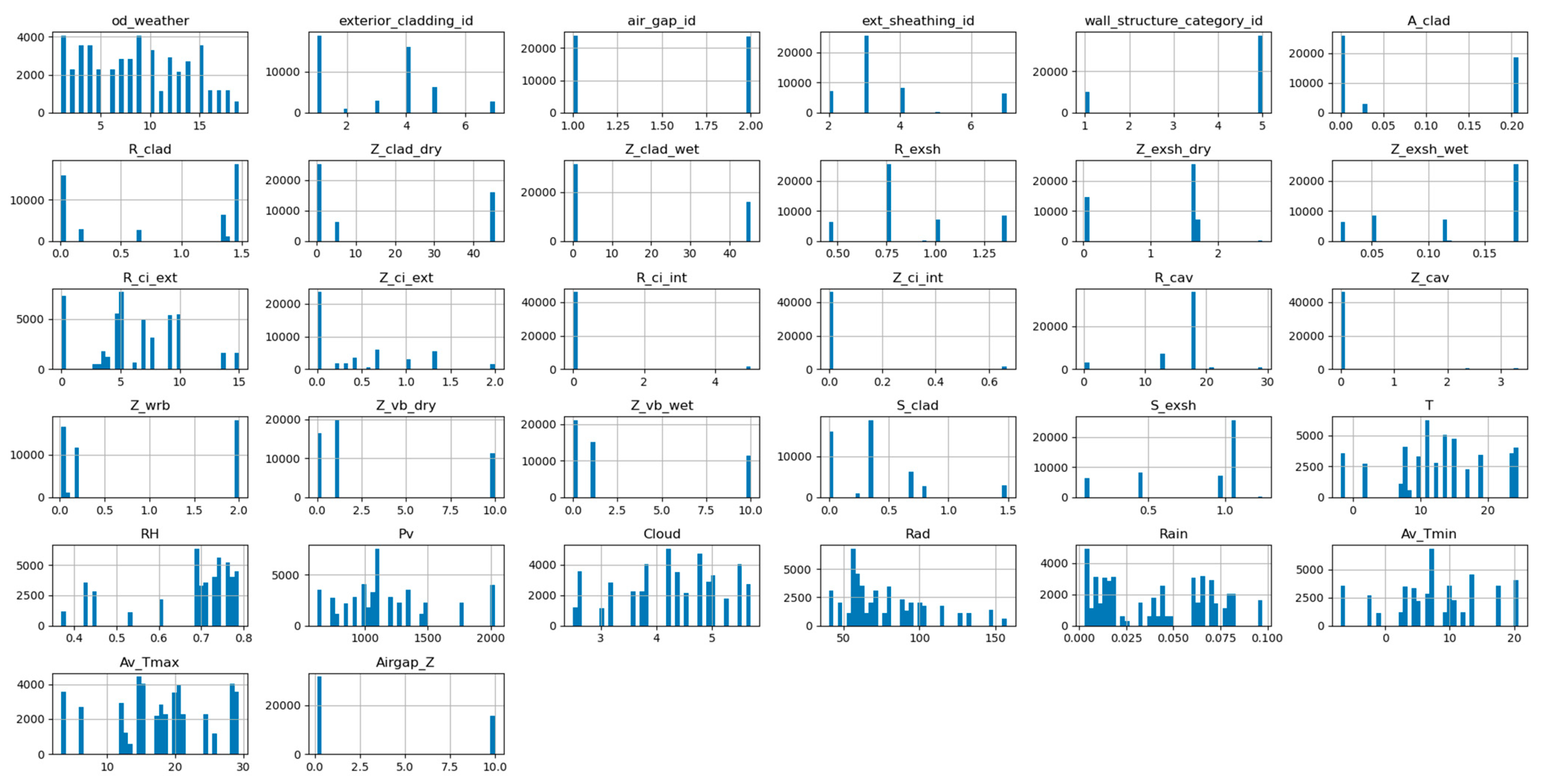
Figure 8 shows the histogram of different input features used for the ML model to predict the mold index. Most weather inputs are widely scattered between the minimum and the maximum values. Some of the inputs are concentrated on several values, such as the vapor resistance of the vapor barrier (Z_vb_wet) and the thermal resistance of the continuous insulation on the interior side of the wall (R_ci_int). The histograms help identify which inputs would require refinements to improve the ML predictions. Ideally, we would want the distribution of values to be evenly scattered across the range of the property values.

4.7. Machine Learning Analyses for Mold Index and Maximum Moisture Content

A commercially available ML analysis tool (Google AutoML for Tables [26]) was used to evaluate the tabular data. Google Vertex AI and its AutoML require little effort and can be used to create a benchmark case for a data scientist’s development [27]. The caveat is that the system is not free, which makes a case for testing and developing a local model if cost is an issue. Additionally, the system does many tasks without the user’s knowledge, and the methods used in the specific model are not disclosed. The benefit of using AutoML is its ease of use, without setting up any local hardware or software environment. However, the user can evaluate the goodness of the performance with several parameters. Therefore, one can achieve good results by using a plug-and-play setup for the data. The authors will present their local model development in a follow-up paper. The AutoML tool conducts several ML tasks behind the scenes:

• Preprocessing the data;
• Performing automatic feature engineering;
• Model architecture searching;
• Model tuning;
• Cross-validating;
• Automatic model selection and ensembling.

Four steps were followed to train and test the ML models. First, the tool trained the ML models to predict the mold index and the maximum moisture content using a data set of simulated results. Second, we tested the performance of the models using the model to predict the performance of new materials that were not part of the training set. Third, the predictions for new climates were tested with materials that were already part of the training set. Fourth, the performance of the ML models was tested with both the new climates and the new materials.

4.7.1. Training the Machine Learning Model

A data set of 48,855 lines of simulated values was used to train the ML tool. The default 80%/10%/10% random split was used (training/validation/test). The prediction was optimized for residual mean squared error (RMSE) with mold index as the target.

Table 6. Calculated accuracies for the mold index and maximum moisture content prediction.

Prediction Target	MAE	RMSE	R2
Maximum mold index	0.024	0.058	0.997
Maximum moisture content	0.154	0.568	0.995

lists the mean absolute error (MAE), RMSE, and coefficient of determination (R²) for predicting the maximum mold index and the maximum moisture content.

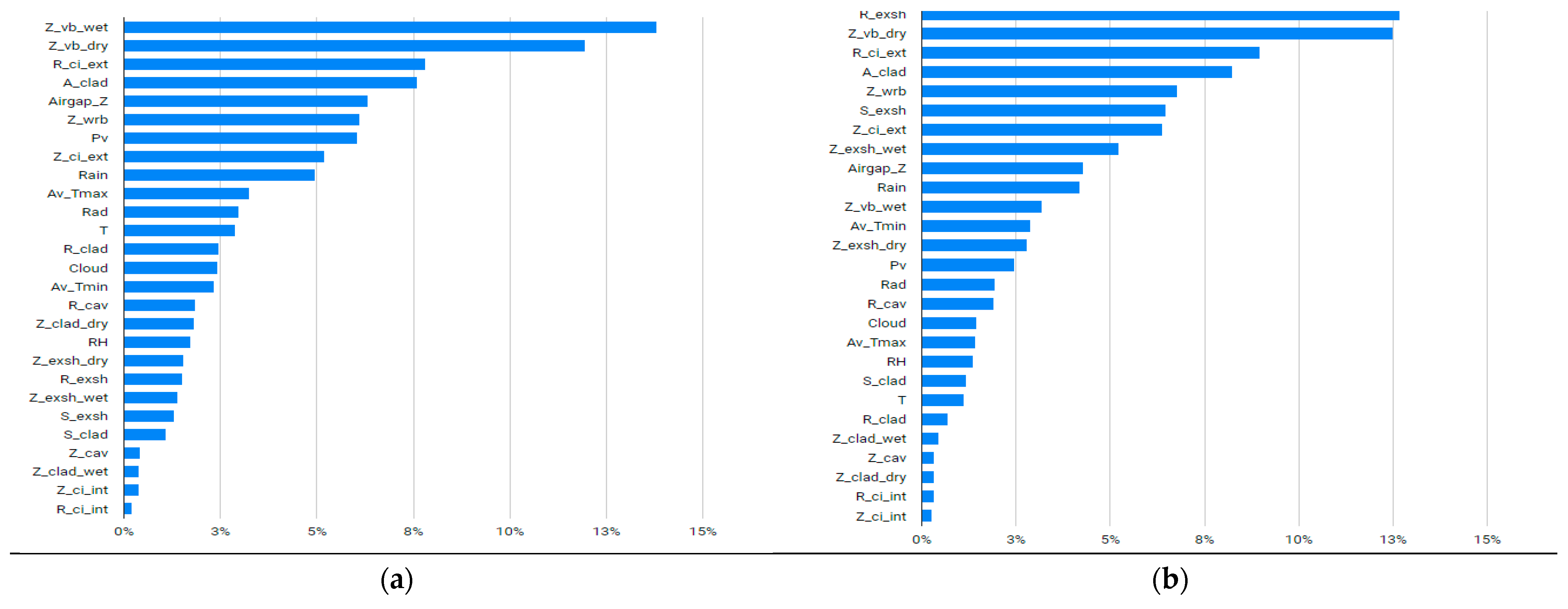
The features in the input data are shown in the order of importance in Figure 9 as determined by the ML tool. The definitions of the parameters are listed in Table 5. The most important features in determining the mold index in the walls are the water vapor resistance (1/permeance) of the vapor barrier (Z_vb_wet and Z_vb_dry) and the thermal resistance of the continuous insulation (R_ci_ext), which are in the top three for predicting the maximum moisture content. However, the thermal resistance of the exterior sheathing is now the most important feature for determining maximum moisture content. Otherwise, the features are in a similar order for the mold index and maximum moisture content predictions, with slight changes in the order of importance.

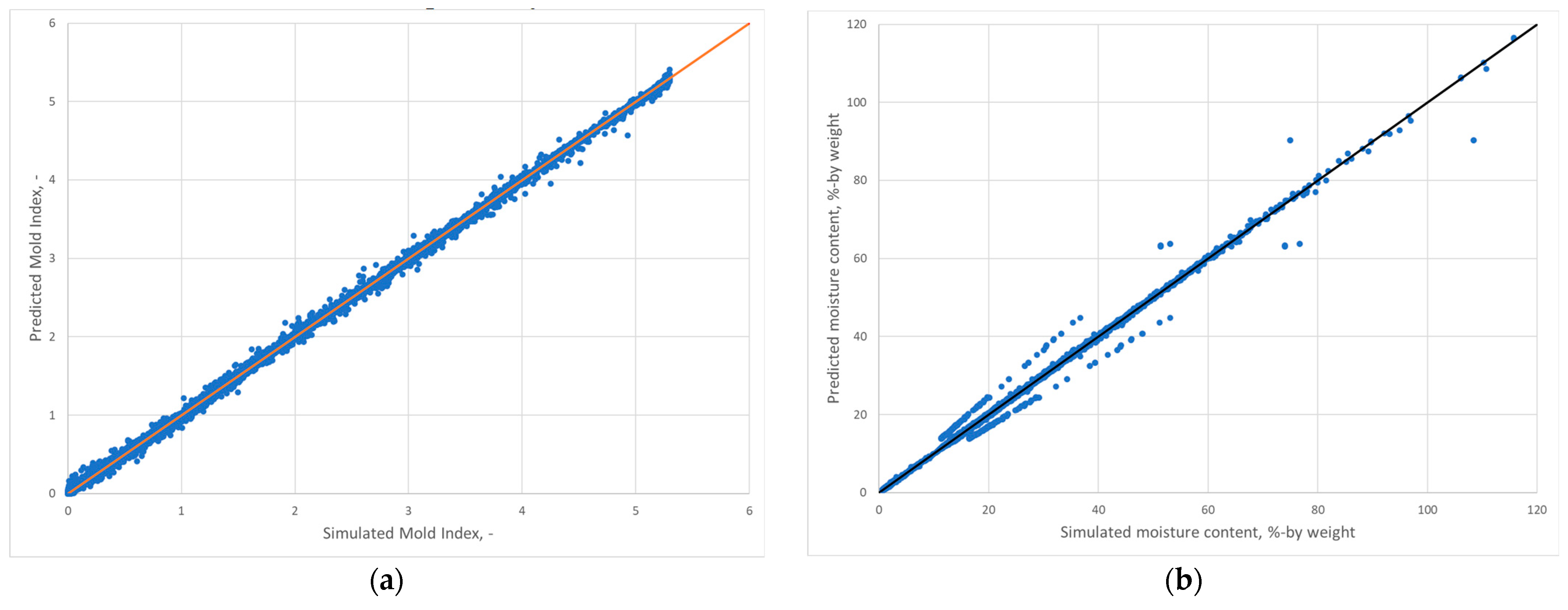
The predicted values from ML models for the mold index and moisture content are depicted vs. the simulated values from hygrothermal simulation tools in Figure 10a,b, respectively. In contrast to the mold index, the moisture content has sections where some of the simulated and predicted values diverge at moisture contents greater than 15%. Despite the divergence, the correlation seems strong, as reflected by R² values of 0.997 and 0.995, respectively.

4.7.2. Predicting the Performance Parameters with New Materials

Two new materials, chipboard exterior sheathing and wood fiber exterior insulation, were introduced, and simulation cases with those materials were carried out. Figure 11 shows the correlation between the ML-predicted and simulated mold index and maximum moisture content for the new materials.

Table 7. Calculated accuracies for the mold index and maximum moisture content prediction for new materials with existing climates in training.

Prediction Target	MAE	RMSE	R2
Mold index	0.134	0.210	0.974
Maximum moisture content	1.940	2.716	0.977

lists the performance indicators. The method predicts these new materials well with no outliers. The results are well correlated with the input data with R-squared over 0.97 both for the mold index and maximum moisture content predictions and the MAE and RMSE representing less than 5% error from the maximum values. However, at high moisture contents >20% by weight, the predictions show consistently higher than simulated moisture contents, and the errors in the predictions are concentrated in this range. This is possibly due to fewer input data being available in ML training with high moisture contents and the highly nonlinear nature of sorption isotherms. The 20% by weight moisture content or higher for wooden materials is considered unacceptable, so both the simulations and the ML predictions predict unacceptable performance.

4.7.3. Predicting the Performance with New Climates

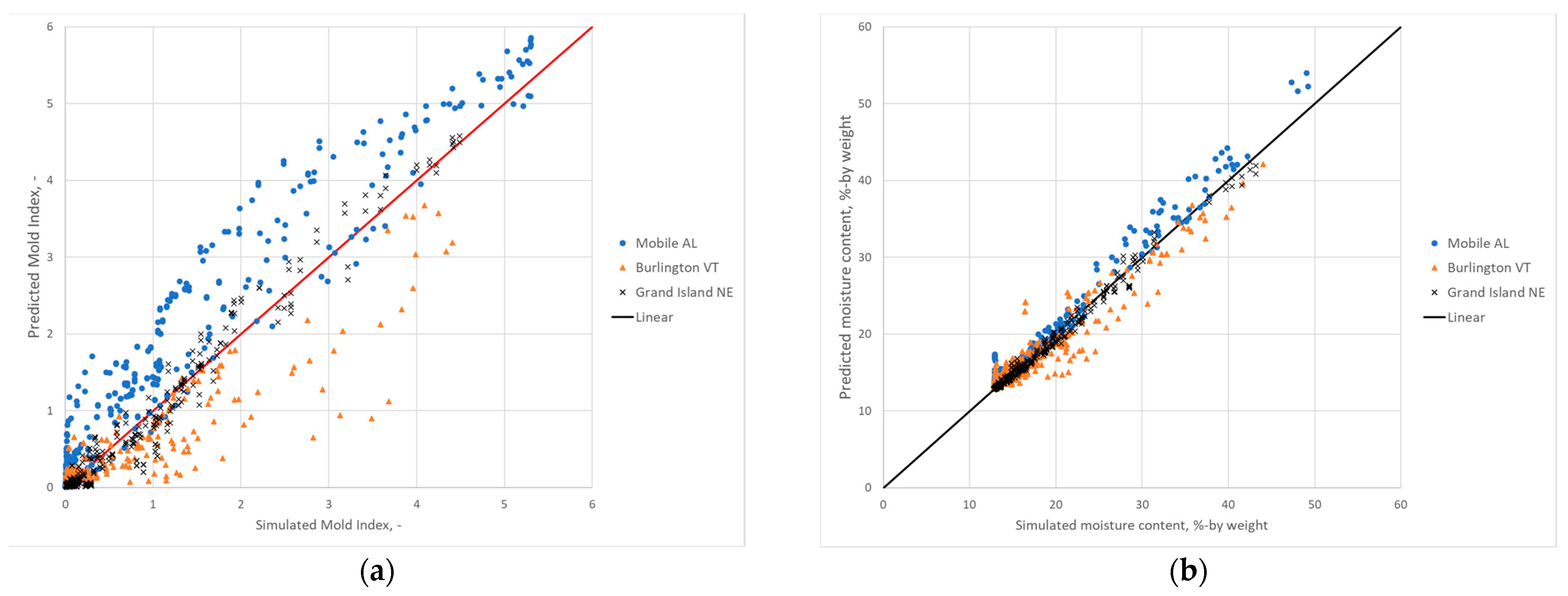
Three new climates—Mobile, Alabama, Burlington, Vermont, and Grand Island, Nebraska—were introduced into the simulations with materials that were included in the training set for ML. Figure 12 shows the correlations for the predicted mold index and maximum moisture content as a function of the simulated values.

Table 8. Calculated accuracies for the mold index and maximum moisture content prediction for new climates with existing materials in training.

Prediction Target	MAE	RMSE	R2
Mold index	0.238	0.420	0.901
Maximum moisture content	0.697	1.270	0.960

shows the performance indicators. The quality of the predictions is worse for the mold index, with both the MAE and RMSE higher and the R² lower for the new climate prediction than for testing with the new materials. The three climates also have different trends: the predictions for Mobile, Alabama, are generally on the high mold index and moisture content side, whereas in Burlington, Vermont, the results are mostly on the low side. Burlington is one of the coldest climates in the data set, and small changes in material and weather parameters can cause large differences in performance. Therefore, more focus should be placed on the extreme climates in the simulations that provide the input data. The ML model predicts maximum moisture content better than the mold index with the new climates.

The performance with weather parameters for Mobile, Alabama, and Grand Island, Nebraska, is conservative and provides safe guidance regarding mold growth by mainly predicting a higher mold index than simulated. However, for Burlington, Vermont, the predictions for the mold index are lower than those simulated, giving a false sense of moisture safety for the wall design. The predictions for the maximum moisture content are similarly low for Burlington, Vermont, but align much better with the simulated data. The poor performance in predicting the mold index in one of the climates indicates that more work is needed to improve the accuracy with new climate locations by adding new different climates into the training set and investigating potential additional weather parameters and their impact on predictions, although the general trend is acceptable.

4.7.4. Predicting Performance with New Materials and New Climates

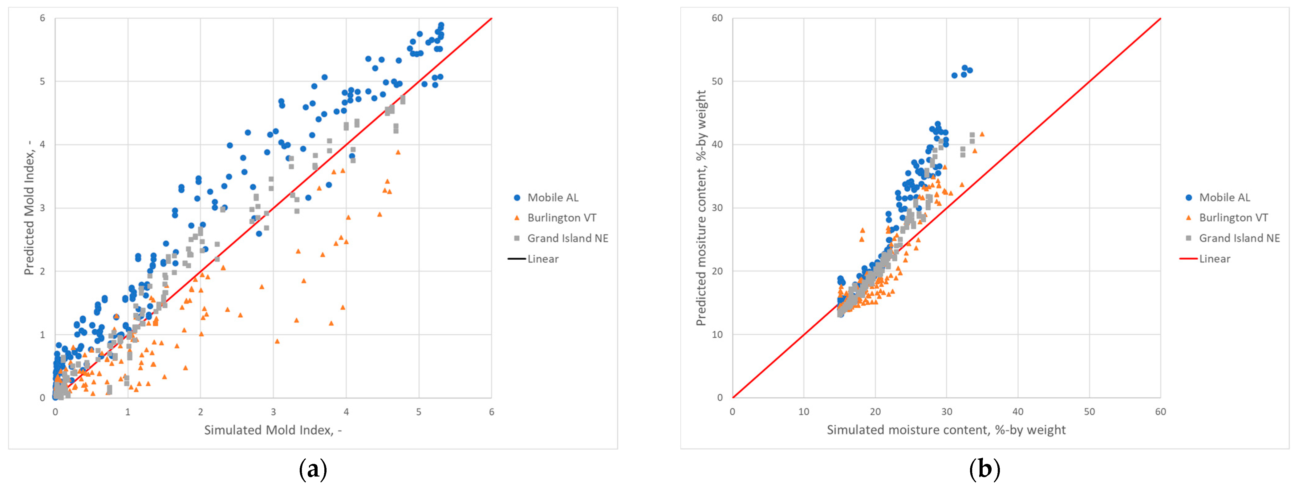
Finally, both the new materials and new climates were introduced together into the simulations, and the performance was predicted with the ML tool. Figure 13 shows the results for wall assemblies, including the two new materials in the three new climates, and

Table 9. Calculated accuracy for the mold index and maximum moisture content prediction for new climates and materials.

Prediction Target	MAE	RMSE	R2
Mold index	0.264	0.449	0.916
Maximum moisture content	2.400	3.413	0.909

shows the performance indicators of the predictions. As expected, the predictions are now worse for MAE and RMSE. On the other hand, R² slightly improved for the mold index prediction compared with the predictions with new climates only. Most of the errors in the predictions are caused by the new climates, and closer investigations of weather parameters are needed.

5. Discussion

The benefits of this ML tool are, first, in the early design stages, to guide proper systems before running a detailed evaluation on many systems. Thereby, it can reduce the significant efforts in running hygrothermal analyses. Second, the tool will be the basis for optimizing the durability performance while assessing thermal performance and decarbonization possibilities. The ability to create granularity by interpolating performance as a function of material properties allows for guiding new material development and selections.

This study shows that ML can predict the hygrothermal performance of a building envelope design with reasonable accuracy (R² > 0.90). The results indicate that performance is strongly correlated to the vapor permeance of the vapor barrier and thermal resistance of the continuous insulation layer for the selected envelope design. The dependence of the accuracy on weather data is not as strong, which could explain why the model’s predictive capability was not strong when the ML model was used to predict performance in other climate zones. Regardless, the model needs additional refinement in filling data gaps to address the performance of different assemblies and exposure to different climate zones, which will be the emphasis of future work.

ML is as good as the input data given in training. The current data set still includes large gaps between the high and low values of the input parameters, and many input values have only a few options. The ML methods cannot accurately learn the dependency of the output as a function of the input values unless there are input values in the region where the change in performance occurs. Finding these regions of input values is also part of future work.

The future development of the tool includes guiding the designer by helping to optimize the material layers in the wall assemblies to meet the user’s requirements for thermal, energy, carbon, and moisture performance. The tool would guide the user to select materials and layers that result in a moisture-safe building envelope. Based on the developed ML tool, which uses material properties as inputs for training, we can run multi-objective optimization to select the optimal material that minimizes embodied carbon of the assembly while meeting all the insulation and moisture durability requirements. The tool would guide improving the assembly for better performance in terms of durability, energy losses, and carbon content.

To develop our own ML model, future work may consider testing various regression models to determine the most accurate algorithm instead of using a commercially available automated ML tool. For model training, more aggressive feature extraction will be applied to reduce the amount of redundant data in the input data set, which can help increase the accuracy and generalization of the model. We will also try different weight initialization and fine-tune the learning model, such as the activation function and a number of hidden layers. Commercially available automated ML tools allow quick benchmarking of our ML model.