
Design and Comparative Analysis of Several Model Predictive Control Strategies for Autonomous Vehicle Approaching a Traffic Light Crossing

 ,
, 
Abstract
1. Introduction
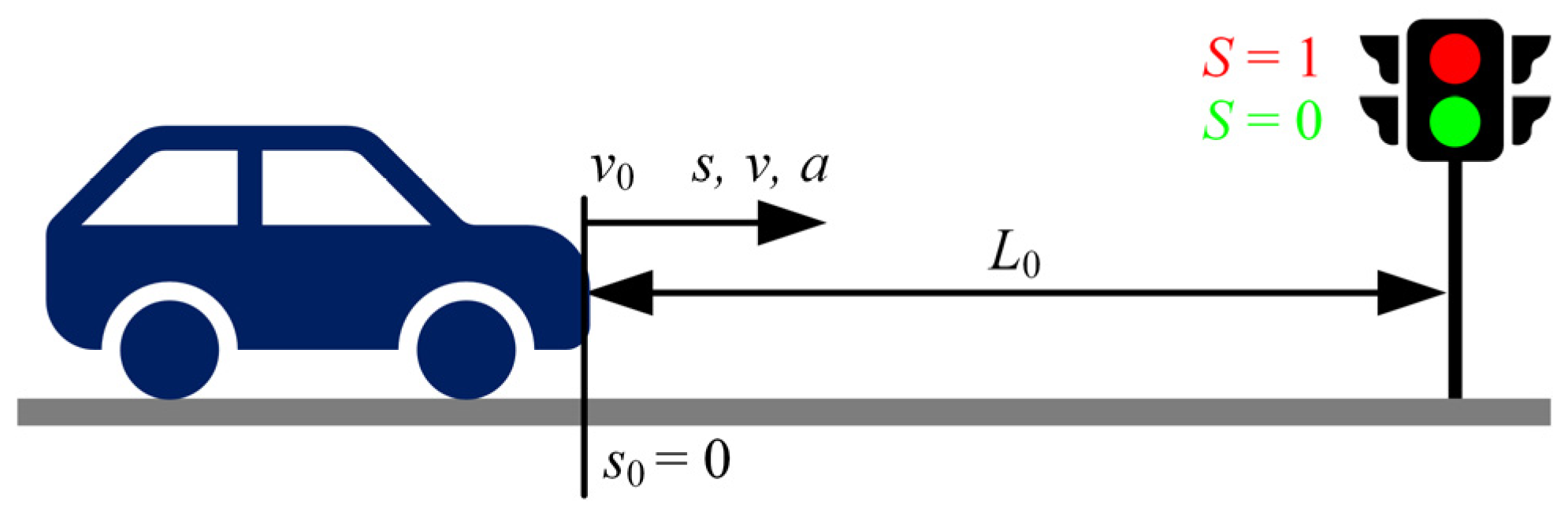
2. Vehicle and Scenario Model
3. Design of Model Predictive Controllers
3.1. Linear Model Predictive Control
3.1.1. Control Law Design
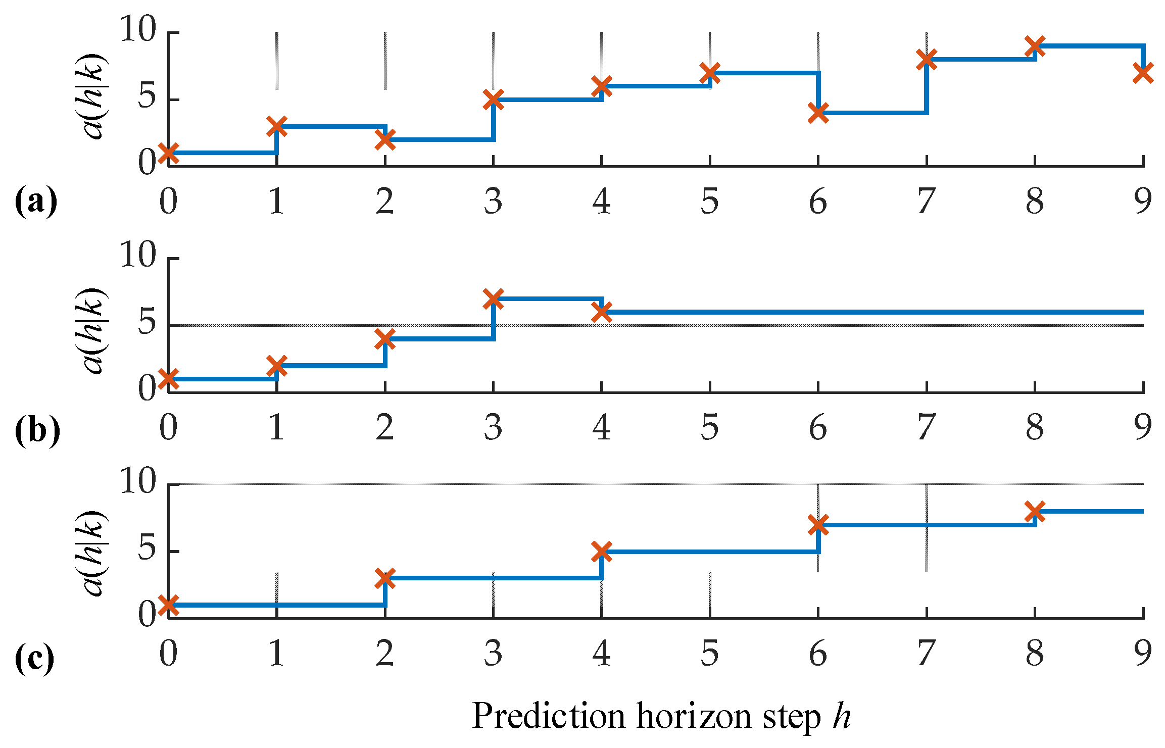
3.1.2. Optimal Control Problem Size Reduction
3.2. Nonlinear Model Predictive Control
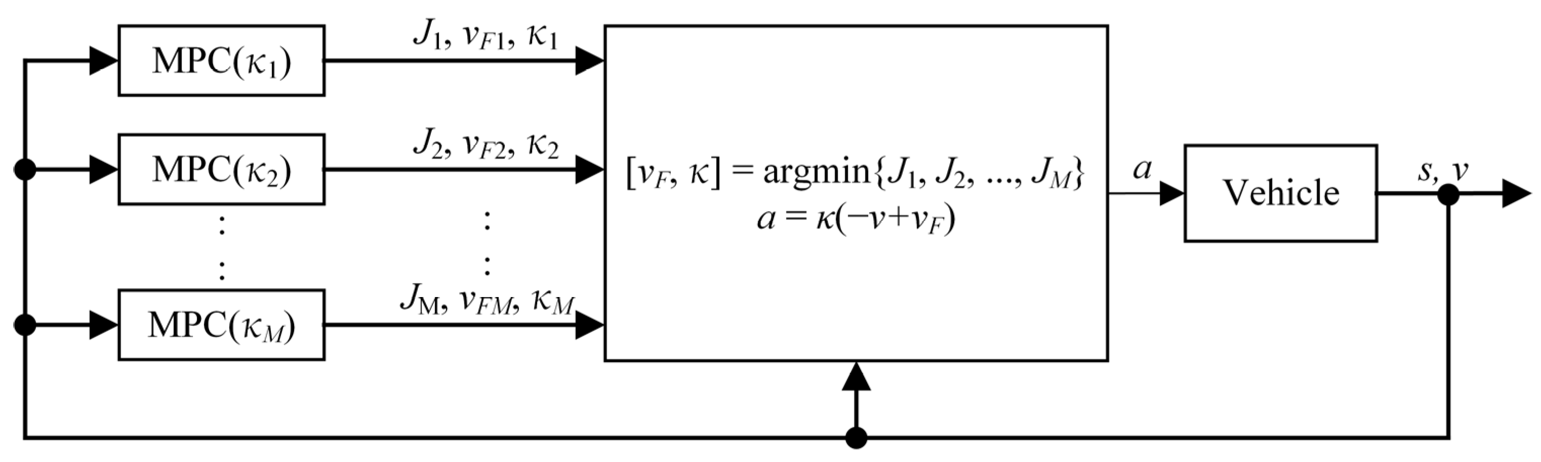
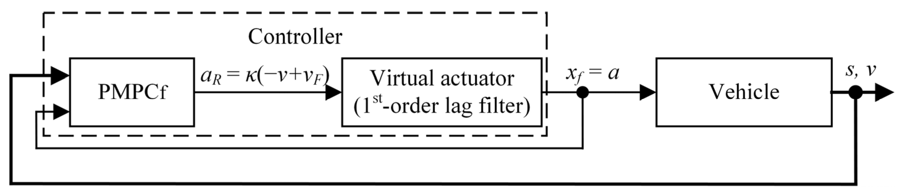
3.3. Parallel Model Predictive Control
4. Simulation Results
4.1. Simulation Setup and Performance Metrics
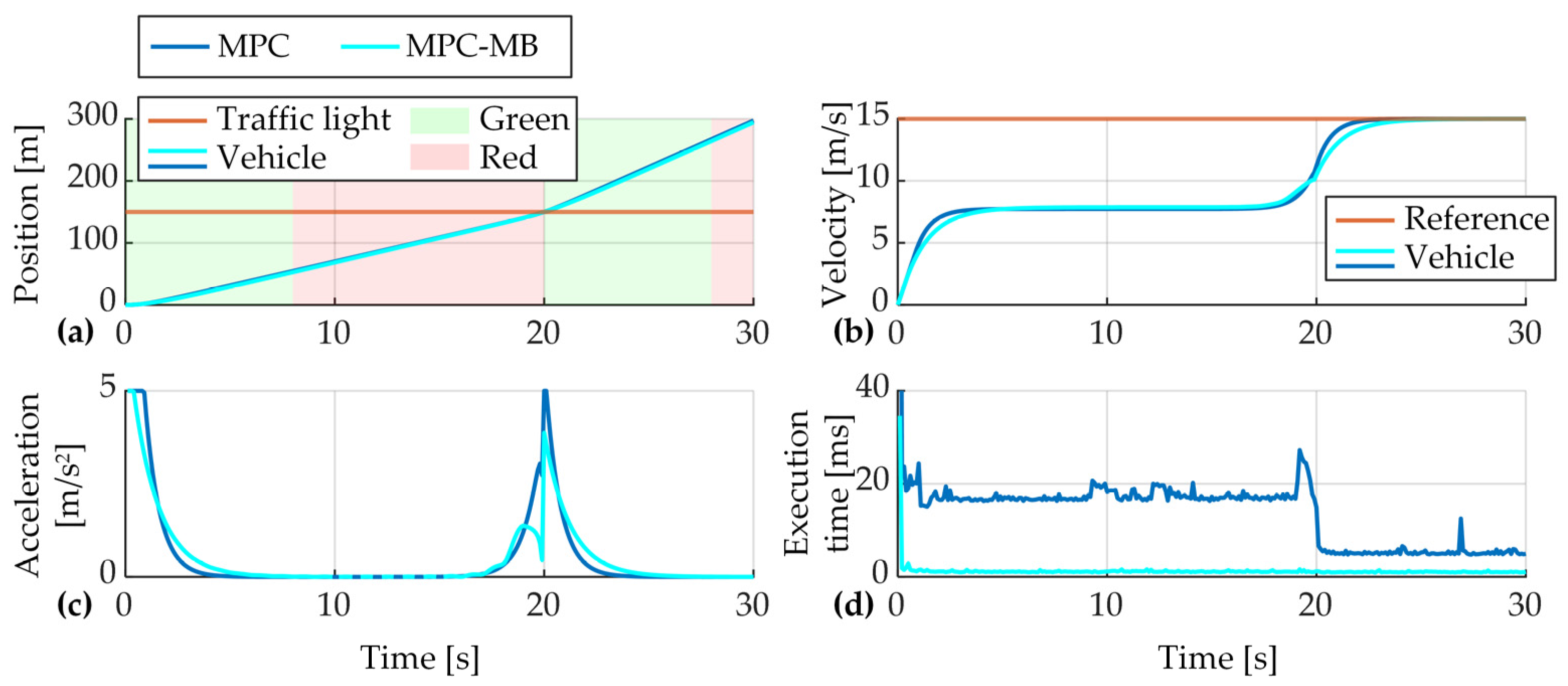
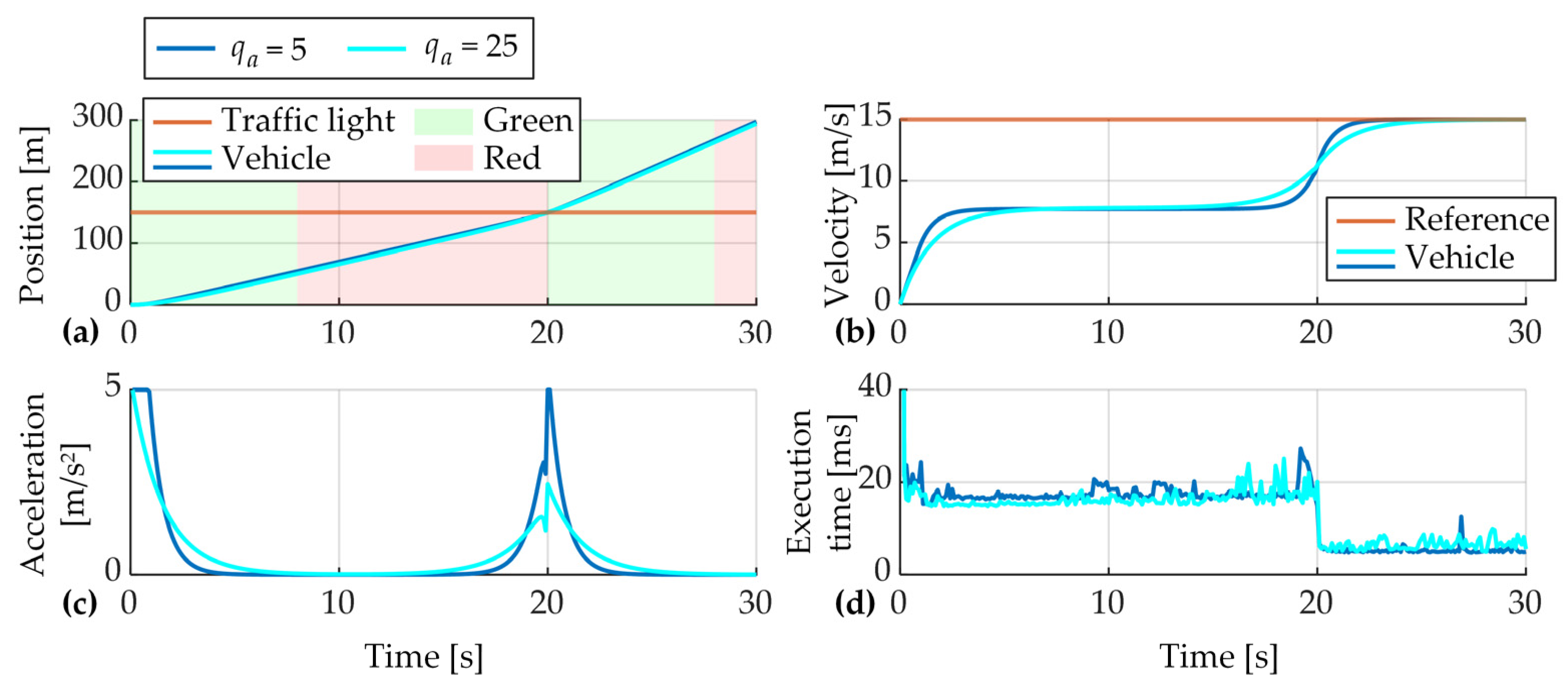
4.2. Linear MPC
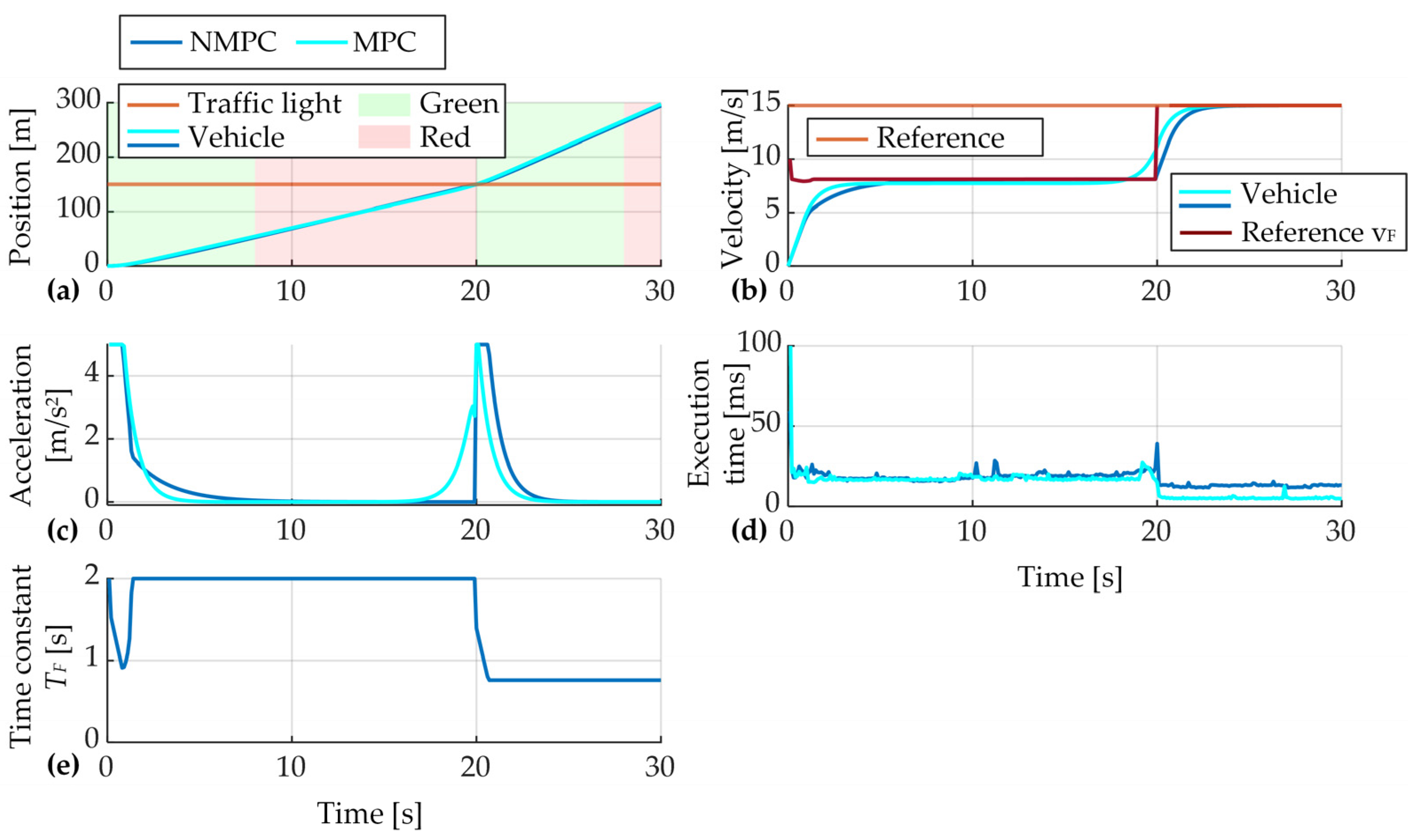
4.3. Nonlinear MPC
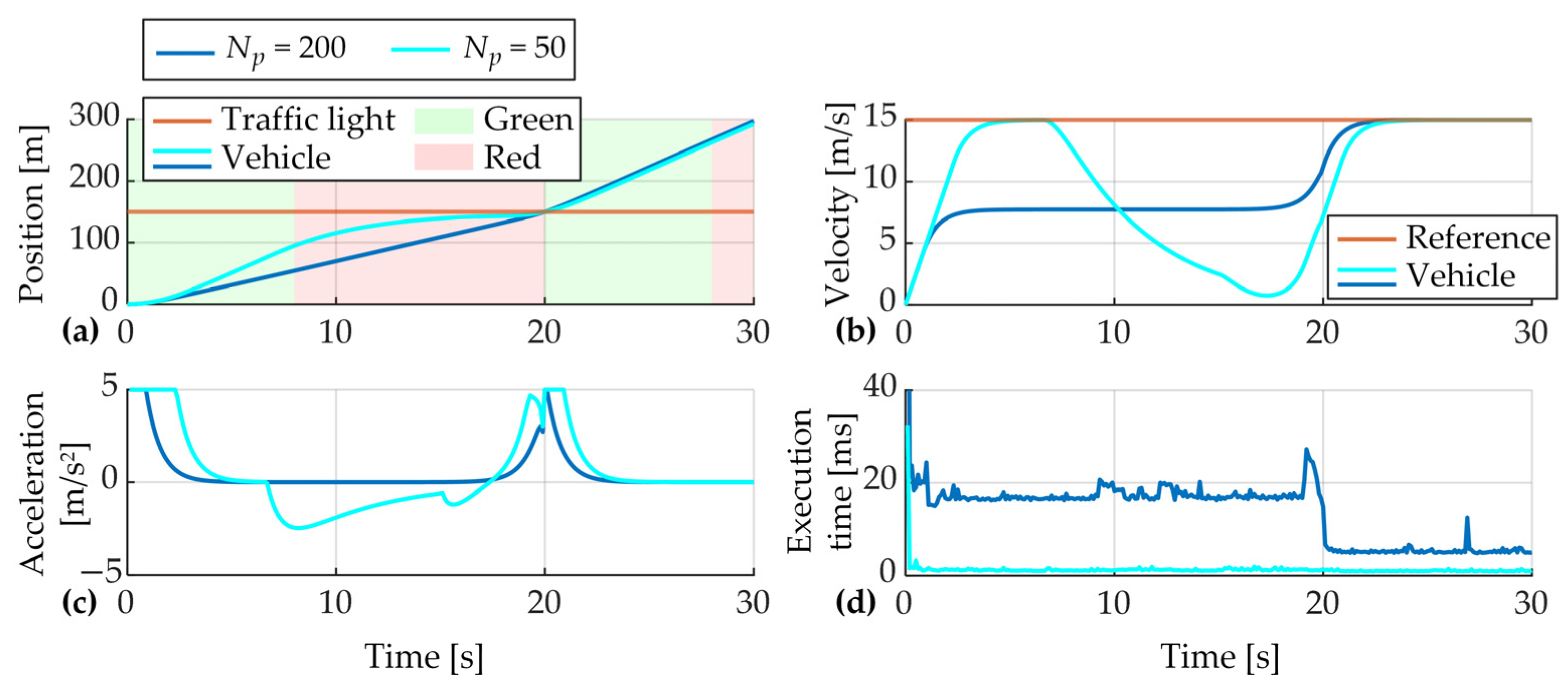
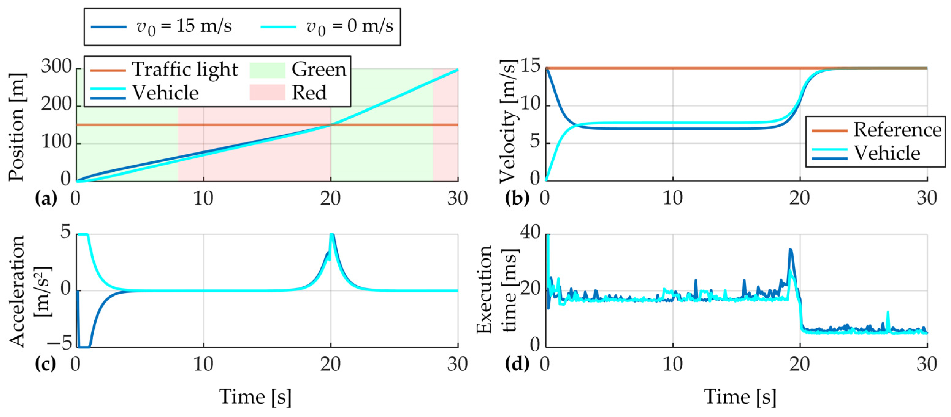
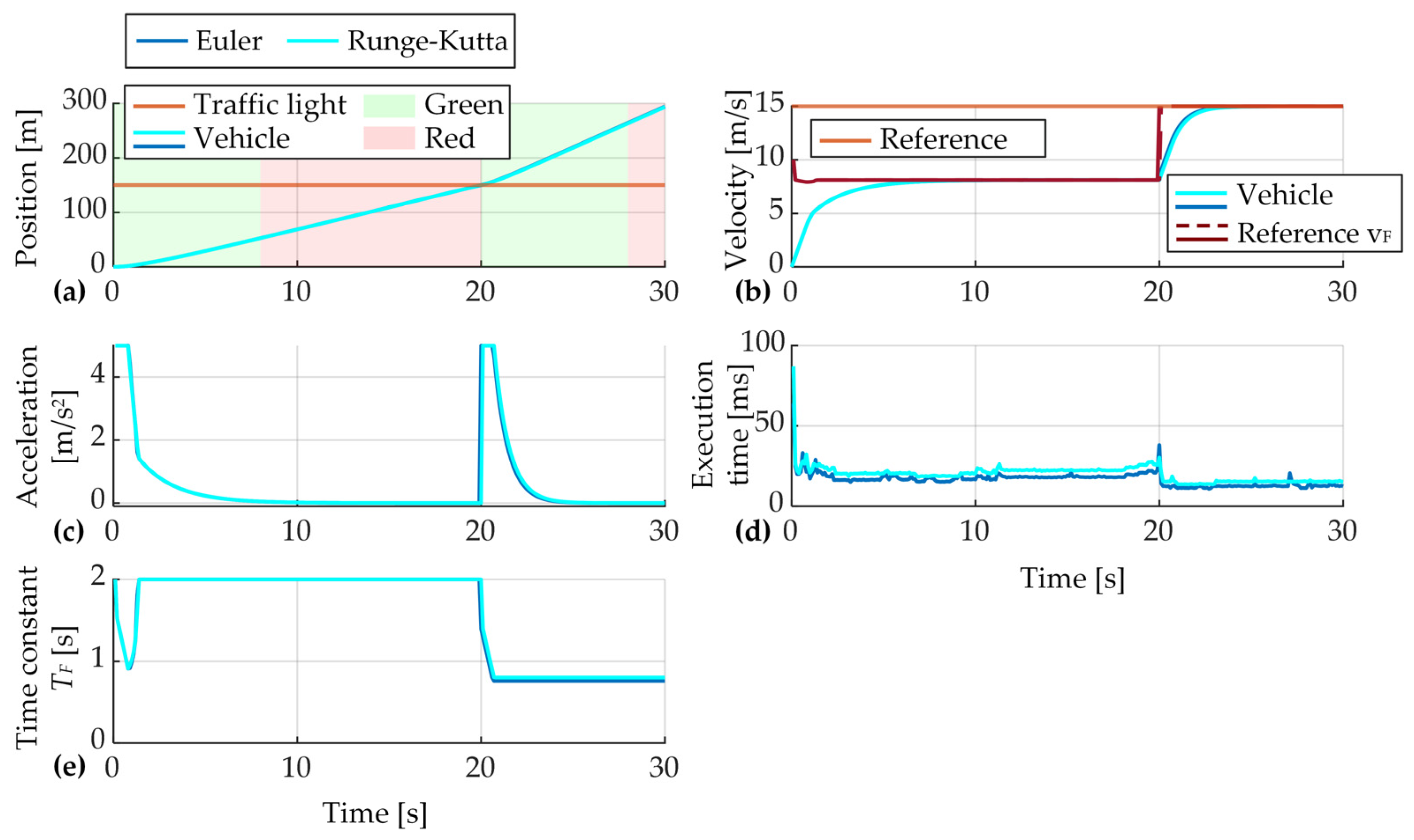
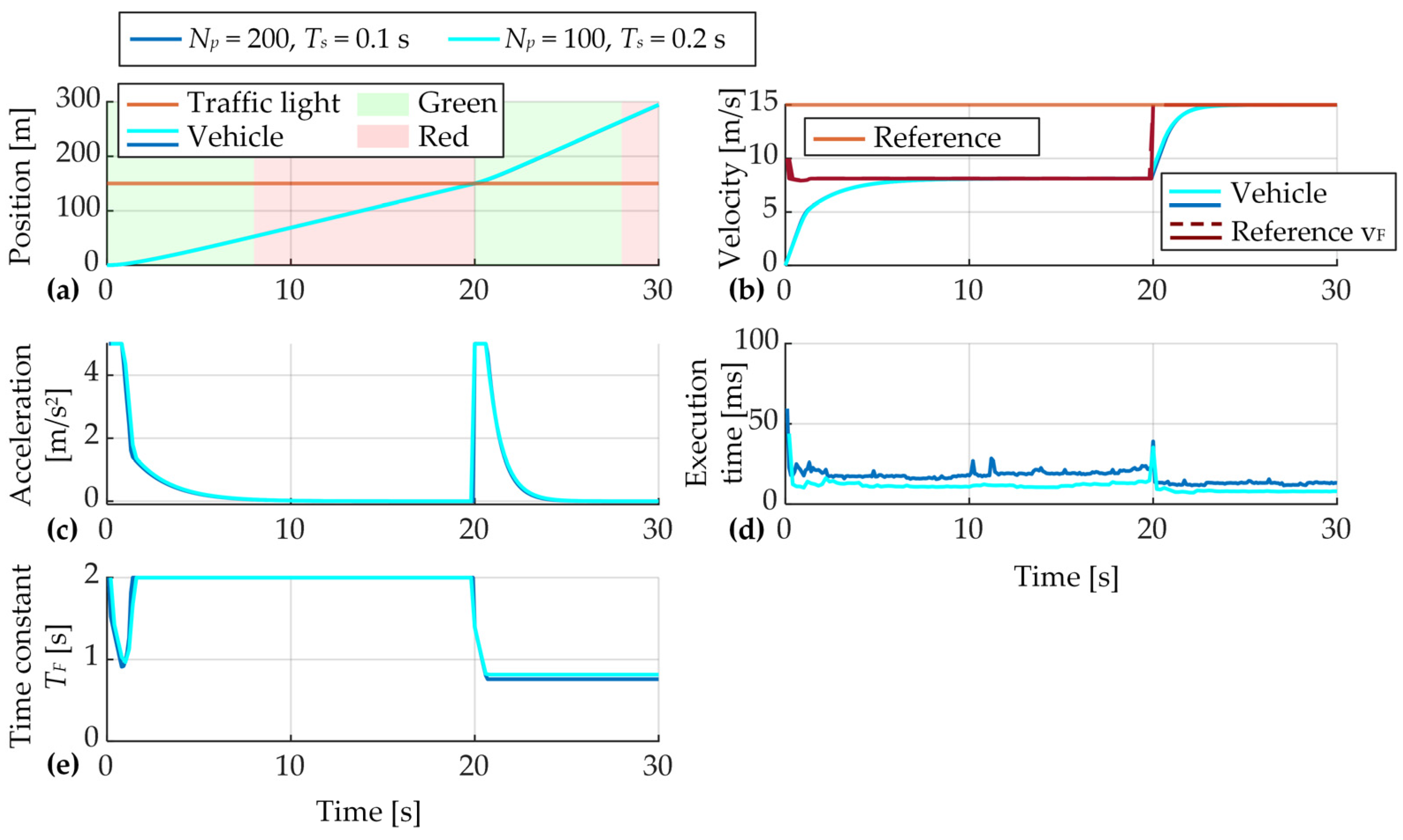
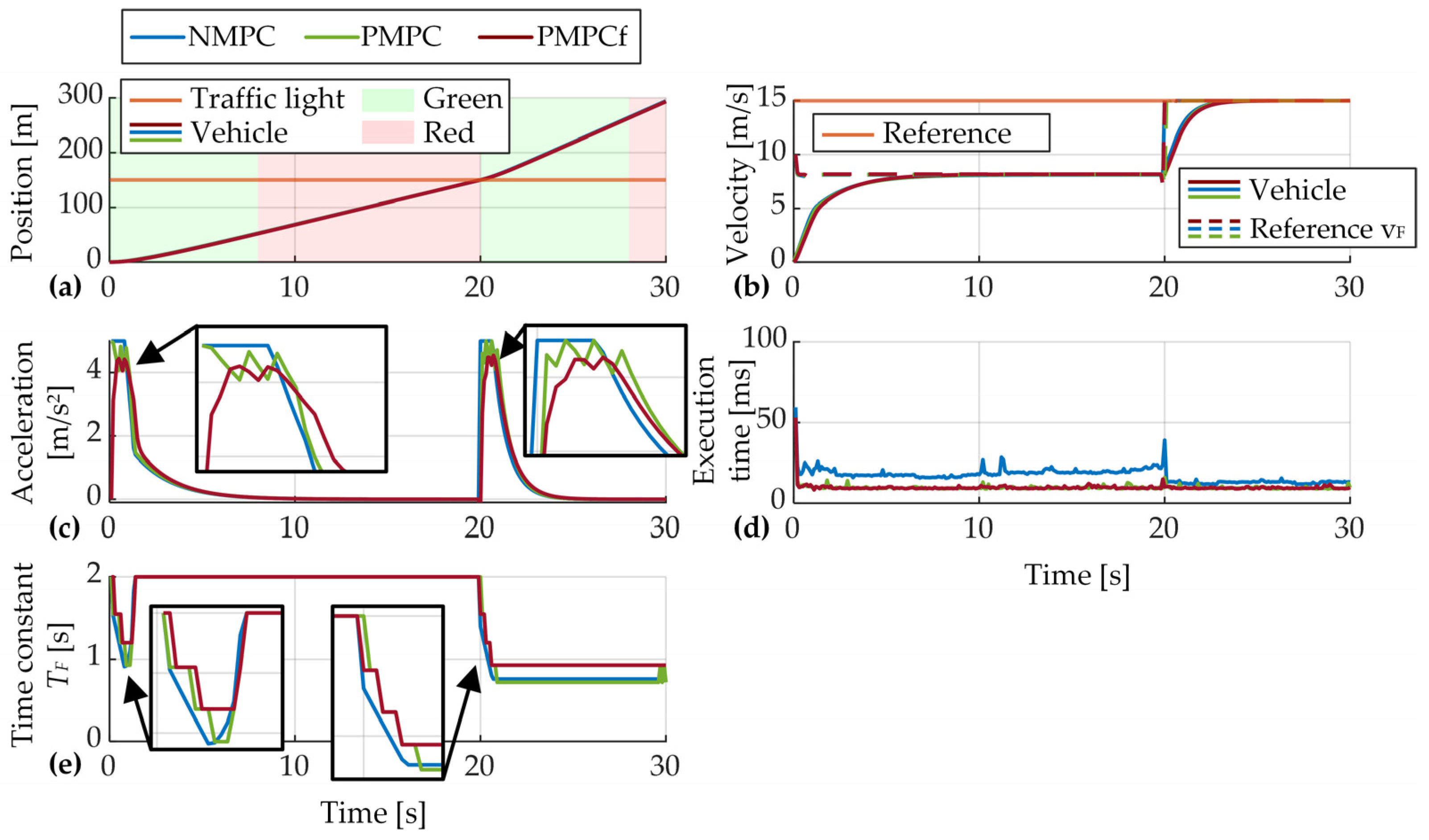
4.4. Parallel MPC
4.5. Comparison of Performance Metrics
5. Discussion
6. Conclusions
Author Contributions
Funding
Data Availability Statement
Acknowledgments
Conflicts of Interest
Abbreviations
| Abbreviation | Meaning |
| AV | Autonomous vehicle |
| MPC | Model predictive control |
| NMPC | Nonlinear model predictive control |
| PMPC | Parallel model predictive control |
| PMPCf | Parallel model predictive control filtered |
| MPC-MB | Move-blocking model predictive control |
| RMS | Root mean square |
| TLS | Traffic light signal |
| QP | Quadratic program |
| GLOSA | Green-light optimal speed advisory |
| LTV | Linear time varying |
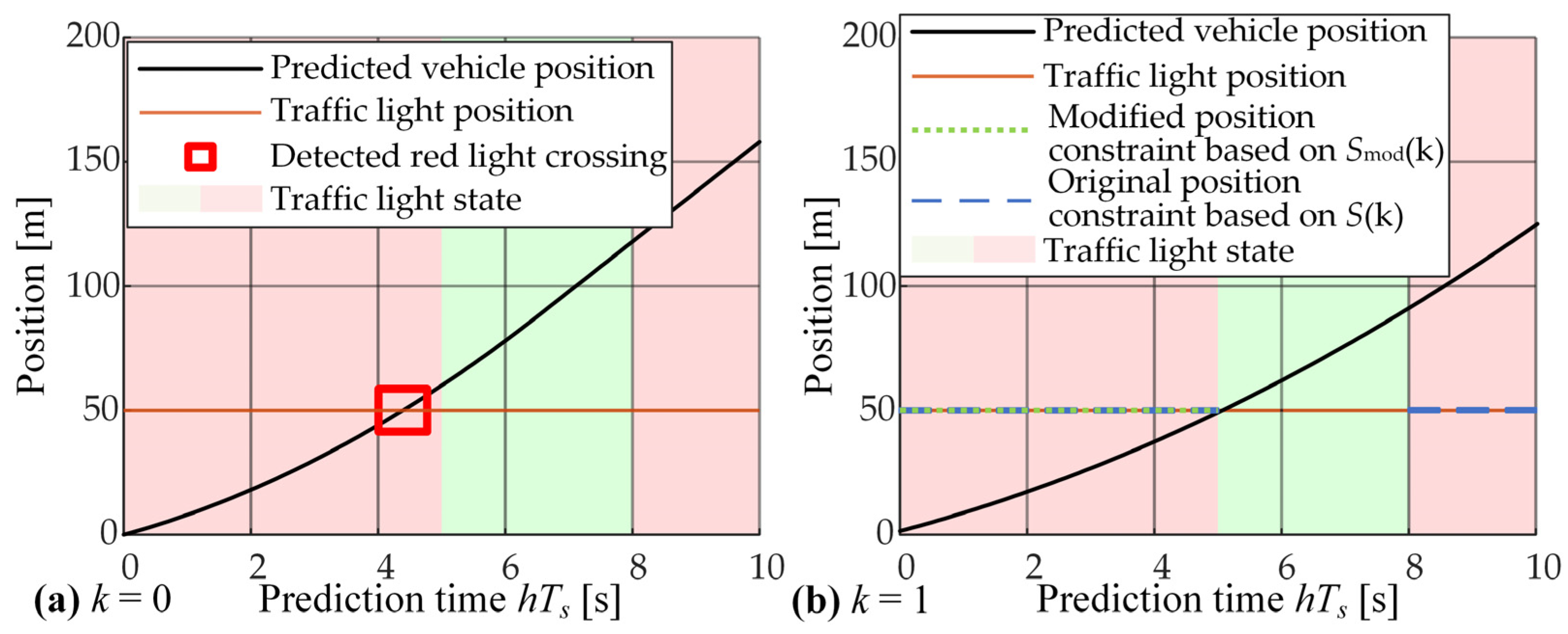
Appendix A. Linear Time-Varying Approach to Traffic-Light-Related Constraint
- Step-Initialize modified traffic light state prediction with actual traffic light state prediction:
- Step-Find the prediction time steps in which the vehicle crossed traffic light in the previous optimization step k − 1 and store the result in vector icross
- Step-Modify the traffic light state for the actual prediction horizon, using the following rules:
- If the vehicle did not cross the traffic light in the previous prediction, i.e., if icross = 0, set the modified traffic light state to the actual one:
- If the vehicle crossed the traffic light, i.e., if icross ≠ 0, find the first step at which the allowed crossing happened hc, i.e., if S(hc|k) = 0 and icross(hc|k) = 1. Modify only the remaining part after the initial allowed crossing step hc:This modification considers all traffic light states after hc to be green, since the vehicle is going to cross during a green light, and all other traffic light states after the vehicle crosses are not relevant.Smod(hc, …, Np − 1|k) = 0
- o
- The special case of hc = 0 indicates that the vehicle just crossed the traffic light and that in the next time step the traffic light state should be considered green.
- o
- In case the crossing is not allowed on the whole prediction horizon (hc is not found), the modified traffic light state prediction remains the same as the actual traffic light state prediction:This means that the vehicle was not able to reach the crossing during the green traffic light phase, or the traffic light was in the red state for the whole duration of the prediction horizon. As soon as the next green traffic light phase is included on the horizon, the vehicle will be able to cross.
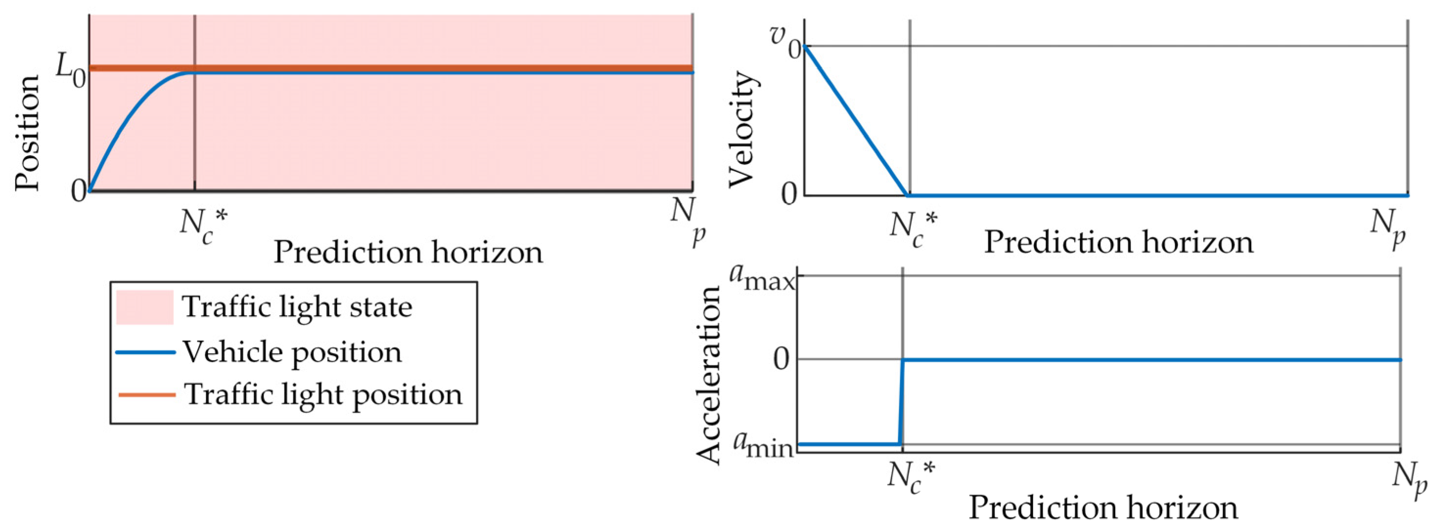
Appendix B. Potential Infeasibility of the QP for Very Short Control Horizons Nc << Np

References
- Texas A&M Transportation Institute 2019 Urban Air Mobility Report. Available online: https://mobility.tamu.edu/umr/report/#methodology (accessed on 15 December 2022).
- Chada, S.K.; Purbai, A.; Gorges, D.; Ebert, A.; Teutsch, R. Ecological Adaptive Cruise Control for Urban Environments Using SPaT Information. In Proceedings of the 2020 IEEE Vehicle Power and Propulsion Conference (VPPC), Gijon, Spain, 18 November–16 December 2020; pp. 2–7. [Google Scholar]
- Mintsis, E.; Vlahogianni, E.I.; Mitsakis, E. Dynamic Eco-Driving near Signalized Intersections: Systematic Review and Future Research Directions. J. Transp. Eng. Part A Syst. 2020, 146, 04020018. [Google Scholar] [CrossRef]
- Lawitzky, A.; Wollherr, D.; Buss, M. Energy Optimal Control to Approach Traffic Lights. In Proceedings of the 2013 IEEE/RSJ International Conference on Intelligent Robots and Systems, Tokyo, Japan, 3–7 November 2013; pp. 4382–4387. [Google Scholar]
- Suzuki, H.; Marumo, Y. Safety Evaluation of Green Light Optimal Speed Advisory (GLOSA) System in Real-World Signalized Intersection. J. Robot. Mechatron. 2020, 32, 598–604. [Google Scholar] [CrossRef]
- Held, M.; Flardh, O.; Martensson, J. Optimal Speed Control of a Heavy-Duty Vehicle in the Presence of Traffic Lights. In Proceedings of the 2018 IEEE Conference on Decision and Control (CDC), Miami, FL, USA, 17–19 December 2018; pp. 6119–6124. [Google Scholar]
- Bouwman, K.R.; Pham, T.H.; Wilkins, S.; Hofman, T. Predictive Energy Management Strategy Including Traffic Flow Data for Hybrid Electric Vehicles. IFAC-PapersOnLine 2017, 50, 10046–10051. [Google Scholar] [CrossRef]
- Bakibillah, A.S.M.; Kamal, M.A.S.; Tan, C.P.; Hayakawa, T.; Imura, J.I. Event-Driven Stochastic Eco-Driving Strategy at Signalized Intersections from Self-Driving Data. IEEE Trans. Veh. Technol. 2019, 68, 8557–8569. [Google Scholar] [CrossRef]
- Asadi, B.; Vahidi, A. Predictive Cruise Control: Utilizing Upcoming Traffic Signal Information for Improving Fuel Economy and Reducing Trip Time. IEEE Trans. Control Syst. Technol. 2011, 19, 707–714. [Google Scholar] [CrossRef]
- Xing, J.; Chu, L.; Guo, C. Optimization of Energy Consumption Based on Traffic Light Constraints and Dynamic Programming. Electronics 2021, 10, 2295. [Google Scholar] [CrossRef]
- Kamalanathsharma, R.K.; Rakha, H.A. Multi-Stage Dynamic Programming Algorithm for Eco-Speed Control at Traffic Signalized Intersections. In Proceedings of the 16th International IEEE Conference on Intelligent Transportation Systems (ITSC 2013), The Hague, The Netherlands, 6–9 October 2013; pp. 2094–2099. [Google Scholar]
- Kamal, M.A.S.; Mukai, M.; Murata, J.; Kawabe, T. Model Predictive Control of Vehicles on Urban Roads for Improved Fuel Economy. IEEE Trans. Control Syst. Technol. 2013, 21, 831–841. [Google Scholar] [CrossRef]
- Uebel, S.; Kutter, S.; Hipp, K.; Schrödel, F. A Computationally Efficient MPC for Green Light Optimal Speed Advisory of Highly Automated Vehicles. In Proceedings of the 5th International Conference on Vehicle Technology and Intelligent Transport Systems, Heraklion, Greece, 3–5 May 2019; pp. 444–451. [Google Scholar]
- Huang, X.; Peng, H. Speed Trajectory Planning at Signalized Intersections Using Sequential Convex Optimization. In Proceedings of the 2017 American Control Conference (ACC), Seattle, WA, USA, 24–26 May 2017; pp. 2992–2997. [Google Scholar]
- Pozzi, A.; Bae, S.; Choi, Y.; Borrelli, F.; Raimondo, D.M.; Moura, S. Ecological Velocity Planning through Signalized Intersections: A Deep Reinforcement Learning Approach. In Proceedings of the 2020 59th IEEE Conference on Decision and Control (CDC), Jeju, Republic of Korea, 14–18 December 2020; pp. 245–252. [Google Scholar]
- Shao, Y.; Sun, Z. Eco-Approach with Traffic Prediction and Experimental Validation for Connected and Autonomous Vehicles. IEEE Trans. Intell. Transp. Syst. 2021, 22, 1562–1572. [Google Scholar] [CrossRef]
- Ozatay, E.; Ozguner, U.; Filev, D.; Michelini, J. Analytical and Numerical Solutions for Energy Minimization of Road Vehicles with the Existence of Multiple Traffic Lights. In Proceedings of the 52nd IEEE Conference on Decision and Control, Firenze, Italy, 10–13 December 2013; pp. 7137–7142. [Google Scholar]
- Meng, X.; Cassandras, C.G. Optimal Control of Autonomous Vehicles for Non-Stop Signalized Intersection Crossing. In Proceedings of the 2018 IEEE Conference on Decision and Control (CDC), Miami, FL, USA, 17–19 December 2018; pp. 6988–6993. [Google Scholar]
- Dong, S.; Chen, H.; Yang, Z.; Liu, Q.; Wang, P. A Hierarchical Strategy for Velocity Optimization of Connected Vehicles with the Existence of Multiple Traffic Lights. In Proceedings of the 2019 Chinese Control Conference (CCC), Guangzhou, China, 27–30 July 2019; pp. 6680–6685. [Google Scholar]
- De Nunzio, G.; De Wit, C.C.; Moulin, P.; Di Domenico, D. Eco-Driving in Urban Traffic Networks Using Traffic Signals Information. Int. J. Robust Nonlinear Control 2016, 26, 1307–1324. [Google Scholar] [CrossRef]
- Mahmoud, Y.H.; Brown, N.E.; Motallebiaraghi, F.; Koelling, M.; Meyer, R.; Asher, Z.D.; Dontchev, A.; Kolmanovsky, I. Autonomous Eco-Driving with Traffic Light and Lead Vehicle Constraints: An Application of Best Constrained Interpolation. IFAC-PapersOnLine 2021, 54, 45–50. [Google Scholar] [CrossRef]
- Mahler, G.; Vahidi, A. An Optimal Velocity-Planning Scheme for Vehicle Energy Efficiency through Probabilistic Prediction of Traffic-Signal Timing. IEEE Trans. Intell. Transp. Syst. 2014, 15, 2516–2523. [Google Scholar] [CrossRef]
- Li, L.; Wen, D.; Yao, D. A Survey of Traffic Control with Vehicular Communications. IEEE Trans. Intell. Transp. Syst. 2014, 15, 425–432. [Google Scholar] [CrossRef]
- Xu, B.; Ban, X.J.; Bian, Y.; Wang, J.; Li, K. V2I Based Cooperation between Traffic Signal and Approaching Automated Vehicles. In Proceedings of the 2017 IEEE Intelligent Vehicles Symposium (IV), Los Angeles, CA, USA, 11–14 June 2017; pp. 1658–1664. [Google Scholar]
- Van Middlesworth, M.; Dresner, K.; Stone, P. Replacing the Stop Sign: Unmanaged Intersection Control for Autonomous Vehicles. In Proceedings of the International Joint Conference on Autonomous Agents and Multiagent Systems, AAMAS, Estoril, Portugal, 12–16 May 2008; Volume 3, pp. 1381–1384. [Google Scholar]
- Jerez, J.L.; Constantinides, G.A.; Kerrigan, E.C.; Ling, K.V. Parallel MPC for Real-Time FPGA-Based Implementation. IFAC Proc. Vol. 2011, 44, 1338–1343. [Google Scholar] [CrossRef]
- Jayaraman, S.K.; Robert, L.P.; Yang, X.J.; Pradhan, A.K.; Tilbury, D.M. Efficient Behavior-Aware Control of Automated Vehicles at Crosswalks Using Minimal Information Pedestrian Prediction Model. In Proceedings of the 2020 American Control Conference (ACC), Denver, CO, USA, 1–3 July 2020; pp. 4362–4368. [Google Scholar]
- Škugor, B.; Deur, J.; Ivanovic, V.; Tseng, H.E. Stochastic Model Predictive Control of Autonomous Vehicles Approaching Unsignalized Crosswalks with Pedestrians. In Proceedings of the European Control Conference, Bucharest, Romania, 13–16 June 2023. submitted for publication. [Google Scholar]
- Xiao, S.; Ge, X.; Han, Q.L.; Zhang, Y. Secure and Collision-Free Multi-Platoon Control of Automated Vehicles under Data Falsification Attacks. Automatica 2022, 145, 110531. [Google Scholar] [CrossRef]
- Maciejowski, J.M. Predictive Control: With Constraints; Prentice Hall: Hoboken, NJ, USA, 2002; ISBN 0201398230. [Google Scholar]
- Andersson, J.A.E.; Gillis, J.; Horn, G.; Rawlings, J.B.; Diehl, M. CasADi: A Software Framework for Nonlinear Optimization and Optimal Control. Math. Program. Comput. 2019, 11, 1–36. [Google Scholar] [CrossRef]
- Ferreau, H.J.; Kirches, C.; Potschka, A.; Bock, H.G.; Diehl, M. QpOASES: A Parametric Active-Set Algorithm for Quadratic Programming. Math. Program. Comput. 2014, 6, 327–363. [Google Scholar] [CrossRef]
- Cagienard, R.; Grieder, P.; Kerrigan, E.C.; Morari, M. Move Blocking Strategies in Receding Horizon Control. In Proceedings of the 2004 43rd IEEE Conference on Decision and Control (CDC), Nassau, Bahamas, 14–17 December 2004; pp. 2023–2028. [Google Scholar]
- Grüne, L.; Pannek, J. Nonlinear Model Predictive Control, 1st ed.; Springer: London, UK, 2011; ISBN 978-0-85729-500-2. [Google Scholar]
- Wächter, A.; Biegler, L.T. On the Implementation of an Interior-Point Filter Line-Search Algorithm for Large-Scale Nonlinear Programming. Math. Program. 2005, 106, 25–57. [Google Scholar] [CrossRef]


| MPC | Overall Cost * J × 105 | Discomfort Index aRMS (m/s2) | Velocity Regulation RMS Error vRMS (m/s) | Traveled Distance smax (m) | Execution Time texe (ms) |
|---|---|---|---|---|---|
| Linear MPC | 1.2007 | 1.2661 | 5.1137 | 295.8402 | 13.9 |
| MPC-MB | 1.2081 (+0.6%) | 1.0956 (−13.5%) | 5.2070 (+1.8%) | 293.0414 (−0.9%) | 1.2 (−91.4%) |
| NMPC | 1.2210 (+1.7%) | 1.3437 (+6.1%) | 5.2136 (+2.0%) | 292.8537 (−1.0%) | 16.3 (+17.3%) |
| PMPC (M = 10) | 1.2286 (+2.3%) | 1.3132 (+3.7%) | 5.2438 (+2.5%) | 291.9483 (−1.3%) | 9.8 (−29.5%) |
| PMPC (M = 20) | 1.2272 (+2.2%) | 1.3281 (+5.0%) | 5.2413 (+2.5%) | 292.0224 (−1.3%) | 19.1 (+37.4%) |
| PMPCf (M = 10) | 1.2304 (+2.5%) | 1.2009 (−5.1%) | 5.2512 (+2.7%) | 291.7150 (−1.4%) | 9.8 (−29.5%) |
| PMPCf (M = 5) | 1.2365 (+3.0%) | 1.1424 (−9.8%) | 5.2851 (+3.4%) | 290.6967 (−1.7%) | 5.0 (−64.0%) |
Disclaimer/Publisher’s Note: The statements, opinions and data contained in all publications are solely those of the individual author(s) and contributor(s) and not of MDPI and/or the editor(s). MDPI and/or the editor(s) disclaim responsibility for any injury to people or property resulting from any ideas, methods, instructions or products referred to in the content. |
© 2023 by the authors. Licensee MDPI, Basel, Switzerland. This article is an open access article distributed under the terms and conditions of the Creative Commons Attribution (CC BY) license (https://creativecommons.org/licenses/by/4.0/).
Share and Cite
Cvok, I.; Pavelko, L.; Škugor, B.; Deur, J.; Tseng, H.E.; Ivanovic, V. Design and Comparative Analysis of Several Model Predictive Control Strategies for Autonomous Vehicle Approaching a Traffic Light Crossing. Energies 2023, 16, 2006. https://doi.org/10.3390/en16042006
Cvok I, Pavelko L, Škugor B, Deur J, Tseng HE, Ivanovic V. Design and Comparative Analysis of Several Model Predictive Control Strategies for Autonomous Vehicle Approaching a Traffic Light Crossing. Energies. 2023; 16(4):2006. https://doi.org/10.3390/en16042006
Chicago/Turabian StyleCvok, Ivan, Lea Pavelko, Branimir Škugor, Joško Deur, H. Eric Tseng, and Vladimir Ivanovic. 2023. "Design and Comparative Analysis of Several Model Predictive Control Strategies for Autonomous Vehicle Approaching a Traffic Light Crossing" Energies 16, no. 4: 2006. https://doi.org/10.3390/en16042006
APA StyleCvok, I., Pavelko, L., Škugor, B., Deur, J., Tseng, H. E., & Ivanovic, V. (2023). Design and Comparative Analysis of Several Model Predictive Control Strategies for Autonomous Vehicle Approaching a Traffic Light Crossing. Energies, 16(4), 2006. https://doi.org/10.3390/en16042006