Accurate Modeling and Control System Design for a Spherical Radial AC HMB for a Flywheel Battery System

Abstract

Different from common cylindrical magnetic bearings, the spherical radial AC HMB has obvious advantages in suppressing the gyroscopic effect, thus it is very suitable for application in flywheel battery systems. In this study, a precise mathematical model of suspension forces is deduced adopting wide-area and universal modeling theories in detail for the spherical radial AC HMB. Different from the traditional Maxwell tensor method based on a cylindrical two-dimensional coordinate system, the improved Maxwell tensor method based on a spherical coordinate system has a wider range and versatility. Then, the detailed explanation about the accuracy, wide-area and universality are given. Further, based on the model, the control system is designed, which includes the overall schematic, hardware and software designs. Finally, stiffness and performance tests are conducted. The good results of the stiffness tests indicate the error between the proposed model and the force-deflection stiffness test results is less than 2.8%. The good performance test results show that, based on the established model and control system, the rotor will soon return to equilibrium position under the disturbance of vehicle action.

1. Introduction

As a kind of physical battery, flywheel batteries have the characteristics of good environmental adaptability, high work efficiency, wide operating temperature range and other advantages [1,2,3,4,5]. For a magnetic flywheel battery system for vehicles, the gyroscopic effect is particularly serious because of the different driving and road conditions. The bearings of a flywheel battery system must withstand not only the weight of the rotor, but also the gyroscopic force [6,7,8]. The gyroscopic effect is enhanced with the increase in vehicle driving and road complexity, which reduces the stability margin of the flywheel rotor system. Therefore, the flywheel battery system has very high requirements for the design and control of magnetic bearings [9]. A cylindrical magnetic bearing, as a typical representative of a flywheel battery, also has a lot of wide applications in other fields [10,11,12,13,14]. The classical radial AC hybrid magnetic bearing (HMB) has been investigated deeply in [14], which is a typical cylindrical magnetic bearing. However, when the rotor is offset or deflected due to different driving conditions and road conditions of the vehicle, the unbalanced magnetic pull parallel to the rotor shaft will inevitably occur. Furthermore, a spherical radial AC HMB for a magnetic suspension flywheel battery was proposed in [15]. Due to its unique spherical air gap and spherical envelope, the bearing’s performance is superior to that of traditional cylindrical magnetic bearings, and it can suppress the gyro effect.

For precise control of a magnetic bearing-rotor system, it is very important to establish an accurate mathematical model of radial suspension force [16,17,18,19,20,21]. For the spherical radial AC HMB, various methods of accurate modeling have also been developed. A popular modeling method is the equivalent magnetic circuit method, and it has been used successfully for many magnetic bearings and also used for spherical radial AC HMB. A modeling method was proposed in [22], which is superior to the traditional equivalent magnetic circuit method. This method focuses on the compensation of edge flux and leakage flux through accurate magnetic field segmentation. In addition, the error source analysis of suspension force was carried out in [23], and a multi-variable dynamics model with an equivalent magnetic circuit method is proposed, which takes into account four variables including temperature, rotation speed, displacement and current. Although the above methods are accurate and have their own optimization process characteristics, they are relatively complex and not universal. Therefore, a universal, simple and accurate modeling method is urgently needed. In [24], a general and accurate modeling method named Maxwell tensor method was presented, which is specially designed for AC magnetic bearing. Thus, considering that spherical radial AC HMBs are AC magnetic bearings, the Maxwell tensor method can be applied to them. However, reference [24] does not refer to the scope beyond the definition of a cylindrical magnetic bearing. Therefore, the original theory is not necessarily valid, and whether the applied scope in the original theory can be expanded is worth studying. Since the topological structures of magnetic bearings are becoming more and more diverse, a more extensive and universal modeling method should be proposed. How to propose a more wide-area and universal modeling approach suitable for magnetic bearings will be the goal of this paper. At the same time, to verify the effectiveness of the model, it is necessary to design the corresponding effective control system scheme.

In this study, the spherical radial AC HMB is taken as an example, and the mathematical models of suspension forces versus displacement, deflection and current are calculated adopting wide-area and universal modeling theories. The modeling of this method is called the improved Maxwell tensor method, which is different from the traditional Maxwell tensor method which is based on a cylindrical two-dimensional coordinate system. The improved Maxwell tensor method is based on a spherical three-dimensional coordinate system. Compared with the traditional Maxwell tensor method, it applies not only to cylindrical topological structures but also to spherical topology, but not the opposite. Therefore, the proposed approach has a wider range and versatility. Then, the accuracy, wide-area and universality analyses are conducted in a detailed manner. Further, based on the established model, the control system is designed. Finally, the effectiveness of the proposed modeling method and control system are verified by experimental tests.

2. Configuration and Principle

Figure 1 shows the overall structure and magnetic circuits of the spherical radial AC HMB. Superficially, the spherical radial AC HMB proposed in this study is very similar to the classical cylindrical radial AC HMB [14,20,24] in that it is based on this classical structure but is a great improvement and innovation. The specific innovation points are listed as follows: First, because the stator, rotor and air gap of magnetic bearings are spherical structures, the electromagnetic force will continue to point to the spherical center of the rotor no matter whether the rotor is deflected or not. Compared with cylindrical magnetic bearings, such as a cylindrical radial AC HMB, the large interference force generated by electromagnetic force on the rotor can be seriously weakened. Therefore, the proposed spherical radial AC HMB is a valuable improvement and is particularly suitable for a vehicle-mounted flywheel battery. Second, the established mathematical model and the control scheme of magnetic force are quite different because of the dissimilar topological structures. There is an advantage to such magnetic bearings that generate very little electromagnetic force when facing rotor deflection, different from traditional cylindrical magnetic bearings, which usually only calculate the relationship between suspension force and displacement or current. Thus, the relationship between the force and deflection angle of the spherical radial AC HMB is very worthwhile to use. Therefore, in order to improve the control accuracy, the relationship between the force and deflection angle as a model can be added into the control system to realize the dual control of displacement and angle. Third, the magnetization of a permanent magnet is advancement for the realization of the spherical magnetic circuit. Fourth, the magnetic flux leakage can be effectively restrained by the outermost layer of the aluminum magnetic ring, which is designed deliberately.

The magnetic circuit diagram of a spherical radial AC HMB is shown Figure 1b. As shown in Figure 1b, the solid line with an arrow represents the biased flux. Its path is as follows: it starts from the N pole of the permanent magnet, flows through one side of the stator, the spherical air gap, the rotor, the other side of the stator, and finally returns to the S pole of the permanent magnet, forming a closed flux path. It can also be seen in the figure that the dotted lines with arrows represent the control fluxes, forming their own paths in the two stator planes, respectively—that is, a closed flux loop is formed in the stator and corresponding spherical air gap and rotor in the plane of each layer.

The working principle of the spherical radial AC HMB is as follows: Because the stator’s pole envelope surface and rotor envelope surface are spherical, the air gap formed by the stator is different from the special spherical shell structure of the cylindrical air gap of traditional magnetic bearings. This special structure causes the suspension force exerted on the rotor to always point towards the rotor center. It can be seen that the spherical magnetic bearing can obviously eliminate the interference electromagnetic force caused by the rotor eccentricity or deflection caused by the vehicle’s working conditions. Therefore, this kind of magnetic bearing has stronger active disturbance immunity.

3. Mathematical Models

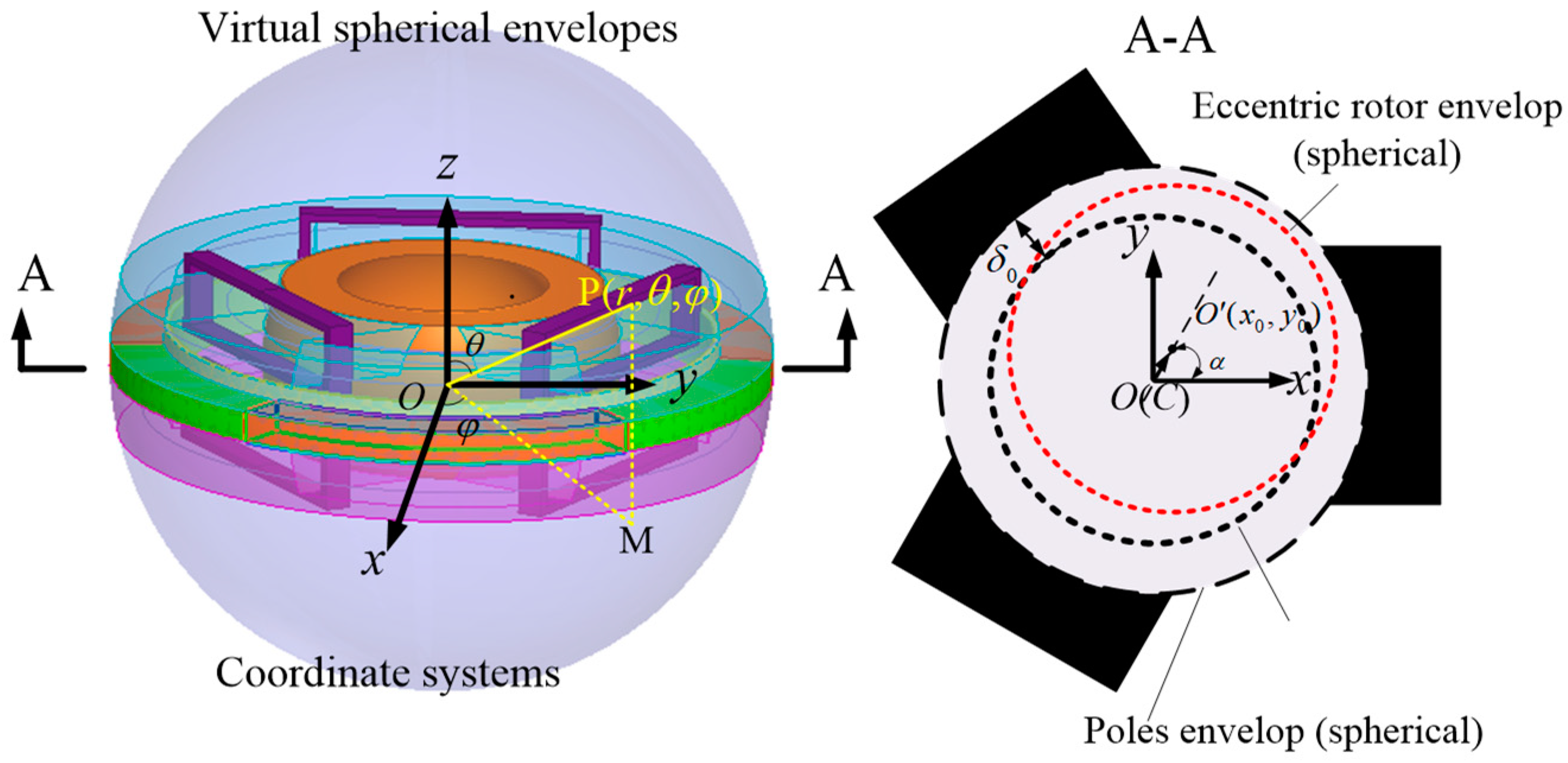
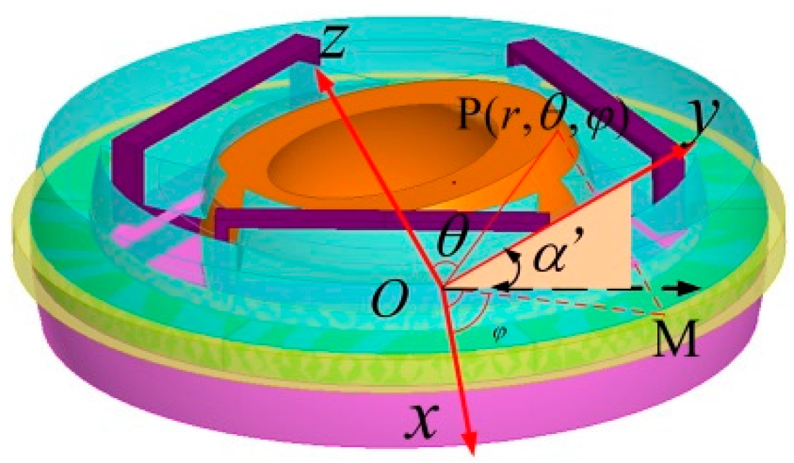
3.1. Coordinate Systems

As shown in Figure 2, since there are two spherical envelope surfaces in the structure, two spherical coordinate systems need to be established: rotor and stator coordinate systems (O-xyz and C-xyz). It is important to note that the centers of these two frames coincide.

Assuming that any point (P) exists on the spherical rotor and its spherical coordinates is P(r,θ,φ). θ is the zenith angle, and φ is the azimuth angle. M is the vertical projection of P points to the radial x-y plane. The transformational relation between the spherical coordinates P(r,θ,φ) and rectangular coordinate system P(x, y, z) are as follows:

$$\{\begin{array}{l}x=r\cdot \sin \theta \cdot \cos \phi \\ y=r\cdot \sin \theta \cdot \sin \phi \\ z=r\cdot \cos \theta \end{array}$$

(1)

3.2. Forces Acting on the Rotor

The main type of centripetal suspension force is Maxwell force, which is mainly determined by biased flux density and control flux density. Therefore, these two key flux densities need to be found. According to the Maxwell tensor method, the Maxwell force per unit area along a certain dimensional mechanical angle on the rotor surface can be expressed as

$$\mathrm{d}F(r,\theta ,\phi )=\frac{B^2(\phi ,t)\cdot \mathrm{d}S}{2{\mu }_0}=\frac{B^2(\phi ,t)}{2{\mu }_0}\cdot r^2\cdot \sin \theta \mathrm{d}\theta \mathrm{d}\phi$$

(2)

The x- and y-components of equations of the Maxwell force (F_x and F_y) are as follows:

$$\{\begin{array}{l}\mathrm{d}{F}_x(r,\theta ,\phi )=\frac{B^2(\phi ,t)\cdot r^2\sin \theta \mathrm{d}\theta \mathrm{d}\phi \sin \theta \cos \phi }{2{\mu }_0}\\ \mathrm{d}{F}_y(r,\theta ,\phi )=\frac{B^2(\phi ,t)\cdot r^2\sin \theta \mathrm{d}\theta \mathrm{d}\phi \sin \theta \sin \phi }{2{\mu }_0}\end{array}$$

(3)

where r is outside diameter of the rotor; μ₀ is permeability of the vacuum.

The biased magnetic flux generated by a permanent magnet is distributed evenly around the circumference if the rotor is in the equilibrium position without eccentricity. Therefore, the magnetic density in the air gap is constant. Once the rotor deviates from the equilibrium position, the originally evenly distributed air gap length distribution will become uneven. Therefore, the flux density in the air gap becomes unstable.

Under the above conditions and with the rotor eccentricity, the expression of the magnetic flux density in the non-uniform air gap B(φ, t) is the key to calculate the Maxwell force. The rotor eccentricity diagram is shown in Figure 2. In Figure 2, x₀ and y₀ are the displacement coordinates of O’ relative to O. δ₀ stands for uniform air gap length when no rotor eccentricity occurs. α is the eccentric angle when no rotor eccentricity occurs in a radial direction and its expression is as follows:

$$\alpha =\arctan (y_0/x_0)$$

(4)

The eccentric direction is defined as the direction in which the length of the air gap becomes minimum. In the universal method, when the rotor is eccentric, the expression is as follows:

$$\epsilon =\frac{\sqrt{x_0{}^2+y_0{}^2}}{{\delta }_0}$$

(5)

where ε stands for the eccentricity ratio.

3.3. Magnetic Flux Density Generated by Control Coils

Without the high-harmonic components, the fundamental component of magnetic motive force generated by control coils is expressed as follows:

$$f_2(\phi ,t)=F_2\cos (\phi -\omega t-\eta )$$

(6)

where F₂ is the fundamental magnetic motive force amplitude generated by control coils. η is the phase angle when time t is 0, and ω is the electrical angle velocity of the current.

Consider that when eccentricity occurs in the rotor, the length expression for the air gap at a mechanical angle φ in the x-y plane is expressed as:

$$\delta (r,\theta ,\phi ,t)={\delta }_0(1-\epsilon \cos (\phi -\alpha ))$$

(7)

When the rotor is eccentric at time t, the flux density generated by the control current at each angle in the air gap is as follows:

$$B_2(\phi ,t)=F_2\cos (\phi -\omega t-\eta )\cdot \frac{{\mu }_0}{2{\delta }_0(1-\epsilon \cos (\phi -\alpha ))}$$

(8)

Symmetrical three-phase AC flows in the symmetrical three-phase coil and can form three-phase magnetic force in the air gap (each phase is a pulsating magnetic force). The amplitude of each phase is equal, and the spacing of phase difference is uniform. A rotating magnetomotive force is then generated by the synthesis of the three-phase pulsating magnetomotive force. In addition, the spherical radial AC HMB adopts centralized windings, and thus the magnetomotive force is almost entirely distributed in the air gap under the magnetic pole, and the leakage flux between the magnetic poles can be ignored.

In Figure 3, the radius of the pole envelope is R, and the pole width is d. Using the two key dimensions, the pole arc angle ($\sigma$) of the spherical radial AC HMB is calculated as 92.86°. The definite means are as follows:

$$\{\begin{array}{l}\sin \sigma =\frac{25}{34.5}=0.7246,\hspace{1em}2\sigma ={92.86}^{\circ }=0.516\mathsf{\pi }\\ \phi = [0,0.516\mathsf{\pi }],[0.67\mathsf{\pi },1.182\mathsf{\pi }],[1.33\mathsf{\pi },1.849\mathsf{\pi }]\end{array}$$

(9)

Then, the amplitude of the three-phase magnetic motive forces generated by three-phase currents (F_2A, F_2B and F_2C) is as follows:

$$\{\begin{array}{l}{F}_{2\mathrm{A}}, \phi \in (0,0.516\mathsf{\pi }); F_{2\mathrm{B}}, \phi \in (0.67\mathsf{\pi },1.182\mathsf{\pi })\\ F_{2\mathrm{C}}, \phi \in (1.33\mathsf{\pi },1.849\mathsf{\pi })\end{array}$$

(10)

$$F_2=\frac{3}{2}{F}_{2\mathrm{A}}=\frac{3}{2}{F}_{2\mathrm{B}}=\frac{3}{2}{F}_{2\mathrm{C}}=\frac{3}{2}\cdot \frac{N_{3}I}{p}$$

(11)

where F₂ stands for the fundamental amplitude of the rotating magnetomotive force generated by the control coils. I stands for the amplitude of the single-phase current. N₃ stands for number of effective single-phase turns of the equivalent three-phase coils. p stands for the pole number of the rotating magnetic field, and its value is 1 for the spherical radial AC HMB.

The amplitude of air gap magnetic flux density generated by the control coil is as follows:

$$B_2=\frac{{\mu }_0\cdot F_2}{2{\delta }_0}$$

(12)

The expression of F₂ is substituted into (12). The quadratic term can be ignored in the calculation because the value of ε is very small.

$$B_2(\phi ,t)=B_2\cos (\phi -\omega t-\eta )(1+\epsilon \cos (\phi -\alpha ))$$

(13)

3.4. Calculation of Magnetic Flux Density Generated by a Permanent Magnet

Some key structural parameters of permanent magnets and the resulting magnetomotive force can be obtained:

$$\{\begin{array}{l}d=\sqrt{{(x_1-x_2)}^2+(y_1-y_2{)}^2+(z_1-z_2{)}^2}\\ {\beta }_{\mathrm{m}}=2\cdot \arcsin \frac{d}{2R_{\mathrm{m}}}\\ F_1=H_{\mathrm{m}}\cdot L_{\mathrm{m}}=H_{\mathrm{m}}\cdot {\beta }_{\mathrm{m}}\cdot R_{\mathrm{m}}\\ =2R_{\mathrm{m}}{H}_{\mathrm{m}}\arcsin \frac{\sqrt{{(x_1-x_2)}^2+(y_1-y_2{)}^2+(z_1-z_2{)}^2}}{2R_{\mathrm{m}}}\end{array}$$

(14)

where F₁ is the magnetic motive force generated by a permanent magnet. H_m is the magnetic field intensity at work point. As shown in Figure 4, each permanent magnet is a section of the spherical envelope. R_m is the radius of the central layer of the spherical envelope of the permanent magnet (equivalent to a spherical envelope). β_m is the central angle of each piece of the permanent magnet. L_m is the equivalent arc length of the permanent magnet in the direction of magnetization. The two endpoints on the equivalent sphere of the permanent magnet are A and B, and their coordinates are A(x₁, y₁, z₁) and B(x₂, y₂, z₂). d is the length of the string between the two points of A and B.

When the rotor is eccentric at a given time t, the air gap flux density generated by the permanent magnet at the mechanical angle θ of the slope can be obtained:

$$B_1(\phi ,t)=F_1\cdot \frac{{\mu }_0}{2\delta (\phi ,t)}=\frac{F_1\cdot {\mu }_0}{2{\delta }_0(1-\epsilon \cos (\phi -\alpha ))}$$

(15)

Then, without the square terms of ε, we can obtain

$$B_1(\phi ,t)=B_1(1+\epsilon \cos (\phi -\alpha ))$$

(16)

The flux density generated by a permanent magnet in the air gap is as follows:

$$B_1=\frac{{\mu }_0{R}_{\mathrm{m}}{H}_{\mathrm{m}}}{{\delta }_0}\cdot \arcsin \frac{\sqrt{{(\Delta x)}^2+(\Delta y{)}^2+(\Delta z{)}^2}}{2R_{\mathrm{m}}}$$

(17)

3.5. Calculation of Force F_x and F_y

According to the principle of air gap magnetic field superposition, the flux density B(φ, t) is as follows:

$$\begin{array}{l}B(\phi ,t)=B_1(\phi ,t)+B_2(\phi ,t)\\ \hspace{1em}\hspace{1em}\hspace{1em}=(1+\epsilon \cos (\phi -\alpha ))\cdot \left(B_1+B_2\cos (\phi -\omega t-\eta )\right)\end{array}$$

(18)

In Figure 5, the radius of the rotor envelope is r and the half axial height is h. Using the two key dimensions, the zenith angle range (θ) can be determined as follows:

$$\{\begin{array}{l}\cos {\theta }_{\min }=\frac{15}{34}=0.4412\\ {\theta }_{\min }={63.82}^{\circ }, {\theta }_{\max }={116.18}^{\circ }\\ \theta =[{63.82}^{\circ },{116.18}^{\circ }]=[0.3545\mathsf{\pi },0.6455\mathsf{\pi }]\end{array}$$

(19)

Then, the components F_x and F_y in the x- and y-axes are as follows:

$$\{\begin{array}{l}{F}_x={\displaystyle \underset{\mathrm{D}}{\iint }\frac{B^2(\phi ,t)\cdot r^2\cdot {(\sin \theta )}^2\cdot \mathrm{d}\theta \cdot \mathrm{d}\phi \cdot \cos \phi }{2{\mu }_0}}\\ ={\displaystyle {\int }_0^{0.516\mathsf{\pi }}{\displaystyle {\int }_{0.3545\mathsf{\pi }}^{0.6455\mathsf{\pi }}\frac{B^2(\phi ,t)\cdot r^2\cdot {(\sin \theta )}^2\cdot \cos \phi }{2{\mu }_0}\mathrm{d}\phi \cdot \mathrm{d}\theta }}\\ +{\displaystyle {\int }_{0.67\mathsf{\pi }}^{1.182\mathsf{\pi }}{\displaystyle {\int }_{0.3545\mathsf{\pi }}^{0.6455\mathsf{\pi }}\frac{B^2(\phi ,t)\cdot r^2\cdot {(\sin \theta )}^2\cdot \cos \phi }{2{\mu }_0}\mathrm{d}\phi \cdot \mathrm{d}\theta }}\\ \hspace{1em}\hspace{1em}+{\displaystyle {\int }_{1.33\mathsf{\pi }}^{1.849\mathsf{\pi }}{\displaystyle {\int }_{0.3545\mathsf{\pi }}^{0.6455\mathsf{\pi }}\frac{B^2(\phi ,t)\cdot r^2\cdot {(\sin \theta )}^2\cdot \cos \phi }{2{\mu }_0}\mathrm{d}\phi \cdot \mathrm{d}\theta }}\\ F_y={\displaystyle \underset{\mathrm{D}}{\iint }\frac{B^2(\phi ,t)\cdot r^2\cdot {(\sin \theta )}^2\cdot \mathrm{d}\theta \cdot \mathrm{d}\phi \cdot \sin \phi }{2{\mu }_0}}\\ ={\displaystyle {\int }_0^{0.516\mathsf{\pi }}{\displaystyle {\int }_{0.3545\mathsf{\pi }}^{0.6455\mathsf{\pi }}\frac{B^2(\phi ,t)\cdot r^2\cdot {(\sin \theta )}^2\cdot \sin \phi }{2{\mu }_0}\mathrm{d}\phi \cdot \mathrm{d}\theta }}\\ +{\displaystyle {\int }_{0.67\mathsf{\pi }}^{1.182\mathsf{\pi }}{\displaystyle {\int }_{0.3545\mathsf{\pi }}^{0.6455\mathsf{\pi }}\frac{B^2(\phi ,t)\cdot r^2\cdot {(\sin \theta )}^2\cdot \sin \phi }{2{\mu }_0}\mathrm{d}\phi \cdot \mathrm{d}\theta }}\\ \hspace{1em}\hspace{1em}+{\displaystyle {\int }_{1.33\mathsf{\pi }}^{1.849\mathsf{\pi }}{\displaystyle {\int }_{0.3545\mathsf{\pi }}^{0.6455\mathsf{\pi }}\frac{B^2(\phi ,t)\cdot r^2\cdot {(\sin \theta )}^2\cdot \sin \phi }{2{\mu }_0}\mathrm{d}\phi \cdot \mathrm{d}\theta }}\end{array}$$

(20)

For simplicity, the square terms of ε and B₂ are ignored because their values are too small. The final simplified expression is derived as follows:

$$\{\begin{array}{l}{F}_x=1.0609\frac{r^2}{{\mu }_0}(B_1{B}_2\cos \eta +\epsilon B_1{}^2\cos \alpha )\\ F_y=1.0609\frac{r^2}{{\mu }_0}(B_1{B}_2\sin \eta +\epsilon B_1{}^2\sin \alpha )\end{array}$$

(21)

In (21), the former is a controllable radial suspension force. By adjusting the control current to change the distribution of the magnetic field in the air gap, the radial suspension force can be completely controlled.

3.6. Calculation of Force F_ix and F_iy

According to (12), (16) and (21), using the Clarke transformation of coordinates, controllable radial suspension force (F_ix and F_iy) is expressed:

$$\{\begin{array}{l}{F}_{ix}=\frac{8r^2{\mu }_0{H}_{\mathrm{m}}{R}_{\mathrm{m}}{N}_3}{15{\delta }_0{}^2}\cdot q\cdot i_{xc}\\ F_{iy}=\frac{8r^2{\mu }_0{H}_{\mathrm{m}}{R}_{\mathrm{m}}{N}_3}{15{\delta }_0{}^2}\cdot q\cdot i_{yc}\\ q=\arcsin \frac{\sqrt{{(\Delta x)}^2+(\Delta y{)}^2+(\Delta z{)}^2}}{2R_{\mathrm{m}}}\end{array}$$

(22)

where i_xc and i_yc are the current components on the x and y axes.

Then, it can be further derived as follows:

$$\left[\begin{array}{l}{i}_x\\ i_y\end{array}\right]=\frac{N_3}{N_2}\left[\begin{array}{l}1\hspace{1em}-\frac{1}{2}\hspace{1em}-\frac{1}{2}\\ 0\hspace{1em}\frac{\sqrt{3}}{2}\hspace{1em}-\frac{\sqrt{3}}{2}\end{array}\right]\left[\begin{array}{l}{i}_{\mathrm{A}}\\ i_{\mathrm{B}}\\ i_{\mathrm{C}}\end{array}\right]$$

(23)

where i_A, i_B and i_C are the three-phase control currents. N₂ is the number of effective single-phase turns of an equivalent two-phase coil. i_x and i_y are the control currents translated by a 3/2 coordinate transformation.

$$\frac{N_3}{N_2}=\sqrt{\frac{2}{3}}$$

(24)

$$\left[\begin{array}{l}{i}_x\\ i_y{}_{}\end{array}\right]=\frac{N_3}{N_2}\cdot \left[\begin{array}{l}{i}_{xc}\\ i_{yc}\end{array}\right]$$

(25)

$$\left[\begin{array}{l}{i}_{xc}\\ i_y{}_c\end{array}\right]=\frac{N_2}{N_3}\cdot \left[\begin{array}{l}{i}_x\\ i_y\end{array}\right]$$

(26)

Considering that the total power after transformation is the same as the original total power, the expression of the simple Clarke coordinate transformation in (22) can be modified by a 3/2 coordinate transformation into:

$$\{\begin{array}{l}{F}_{ix}=\frac{\sqrt{3}}{\sqrt{2}}\cdot \frac{8r^2{\mu }_0{H}_{\mathrm{m}}{R}_{\mathrm{m}}{N}_3}{15{\delta }_0{}^2}\cdot q\cdot i_x\\ F_{iy}=\frac{\sqrt{3}}{\sqrt{2}}\cdot \frac{8r^2{\mu }_0{H}_{\mathrm{m}}{R}_{\mathrm{m}}{N}_3}{15{\delta }_0{}^2}\cdot q\cdot i_y\end{array}$$

(27)

3.7. Calculation of Force F_lx and F_ly

In (21), the latter is the Maxwell force generated by the eccentricity of the rotor, which is proportional to the direction of the eccentric rotor and the eccentric distance. The force components F_ix and F_iy of the AC HMB monolithic on the x and y axes can be expressed as follows:

$$\{\begin{array}{l}{F}_{lx}=\frac{1.06r^2{H}_{\mathrm{m}}{}^2{R}_{\mathrm{m}}{}^2{\mu }_0}{{\delta }_0{}^2}\cdot q^2\cdot x\\ F_{ly}=\frac{1.06r^2{H}_{\mathrm{m}}{}^2{R}_{\mathrm{m}}{}^2{\mu }_0}{{\delta }_0{}^2}\cdot q^2\cdot y\end{array}$$

(28)

3.8. Calculation of Force F_xx and F_yy

The spherical radial AC HMB has two stators, and the calculation results just depend on a single stator. In this way, the force is almost twice the calculated result of a single piece.

$$\{\begin{array}{l}{F}_{xx}=\frac{\sqrt{3}}{\sqrt{2}}\cdot \frac{16r^2{\mu }_0{H}_{\mathrm{m}}{R}_{\mathrm{m}}{N}_3}{15{\delta }_0{}^2}\cdot q\cdot i_x+\frac{2.12r^2{H}_{\mathrm{m}}{}^2{R}_{\mathrm{m}}{}^2{\mu }_0}{{\delta }_0{}^2}\cdot q^2\cdot x\\ F_{yy}=\frac{\sqrt{3}}{\sqrt{2}}\cdot \frac{16r^2{\mu }_0{H}_{\mathrm{m}}{R}_{\mathrm{m}}{N}_3}{15{\delta }_0{}^2}\cdot q\cdot i_y+\frac{2.12r^2{H}_{\mathrm{m}}{}^2{R}_{\mathrm{m}}{}^2{\mu }_0}{{\delta }_0{}^2}\cdot q^2\cdot y\end{array}$$

(29)

3.9. Mathematical Models of Magnetic Force versus Deflection Angle

Because of the advantage that such magnetic bearings generate very little electromagnetic force when facing rotor deflection, different from traditional cylindrical magnetic bearings, the relationship between the force and deflection angle for spherical magnetic bearings should be more emphasized. The specific relationship is as follows:

When the rotor is deflected, the magnetic force will point to the rotor center due to the centripetal force, which can reduce the interference force of the stator poles on the rotor. Figure 6 shows the coordinate systems and rotor deflection diagrams.

The expression of centripetal force is as follows:

$$F_r=0.436\frac{{\mu }_0{H}_{\mathrm{m}}{R}_{\mathrm{m}}q}{{\delta }_0{}^{{}^2}}\cdot [2H_{\mathrm{m}}{R}_{\mathrm{m}}q+\sqrt{6}{N}_3\epsilon (\cos \alpha \prime \cdot i_x+\sin \alpha \prime \cdot i_y)]$$

(30)

where α′ is the deflection angle.

3.10. Accuracy Analysis

(1)

During the modeling process for the improved Maxwell tensor method, the Maxwell force is actually determined by the area of the main magnetic flux acting on the rotor, rather than the equivalent area of the magnetic pole adopted by the traditional equivalent magnetic circuit method. Therefore, the proposed method in this paper is direct and accurate to the rotor as the object for force decomposition.

(2)

The traditional equivalent magnetic circuit method cannot be modeled accurately for the irregular magnetic circuit because it is a simple substitution of the equivalent magnetic circuit, and therefore the accuracy of modeling is greatly reduced. However, the method proposed in this paper can modify the value of the magnetomotive force according to the shape of the magnetic circuit so as to ensure the accuracy of the modeling results.

(3)

The traditional Maxwell tensor method based on cylindrical a two-dimensional coordinate system is unable to build the model for a spherical structure of magnetic bearing; nevertheless, the improved Maxwell tensor method based on a spherical three-dimensional coordinate system can establish the model of a cylindrical magnetic bearing. Therefore, the improved Maxwell tensor method is more accurate in building spherical magnetic bearings than using the traditional Maxwell tensor method.

3.11. Wide-Area and Universality Analyses

(1)

Determination of coordinate system

For spherical magnetic bearing-rotor systems, a spherical coordinate system is used. For cylindrical magnetic bearing-rotor systems, a cylindrical coordinate system is used. For cylindrical magnetic bearing-spherical-rotor systems, a spherical coordinate system is used. Thus, the spherical coordinate system suitable for spherical magnetic bearings is a further extension from the two-dimensional coordinate system of cylindrical magnetic bearings to a three-dimensional coordinate system. In other words, the two-dimensional coordinate system of cylindrical magnetic bearings is a special case of a spherical three-dimensional coordinate system. The modeling process for spherical radial AC HMB can reflect the universality and wide-area character of suspension force modeling for AC magnetic bearings.

(2)

Magnetic flux density generated by control coils

Since the Maxwell tensor method is especially suitable for AC magnetic bearing, Equation (12) can be modified according to the number of inverters driving the magnetic bearing.

(3)

Flux density generated by permanent magnet

Permanent magnet components (magnetomotive force and flux density) can be determined according to the topology of a permanent magnet, stator and magnetic pole, that is, Equation (14) can be modified according to the actual magnetic bearing topology.

(4)

Total Maxwell force

The total Maxwell force can be determined according to the number of stators, and Equation (29) can be modified.

In conclusion, the improved Maxwell tensor method is suitable for any topological structure of AC magnetic bearings, and the key steps can be followed to make local modifications. Different from the traditional Maxwell tensor method based on a cylindrical two-dimensional coordinate system, the improved Maxwell tensor method based on a spherical three-dimensional coordinate system has a wider range and versatility.

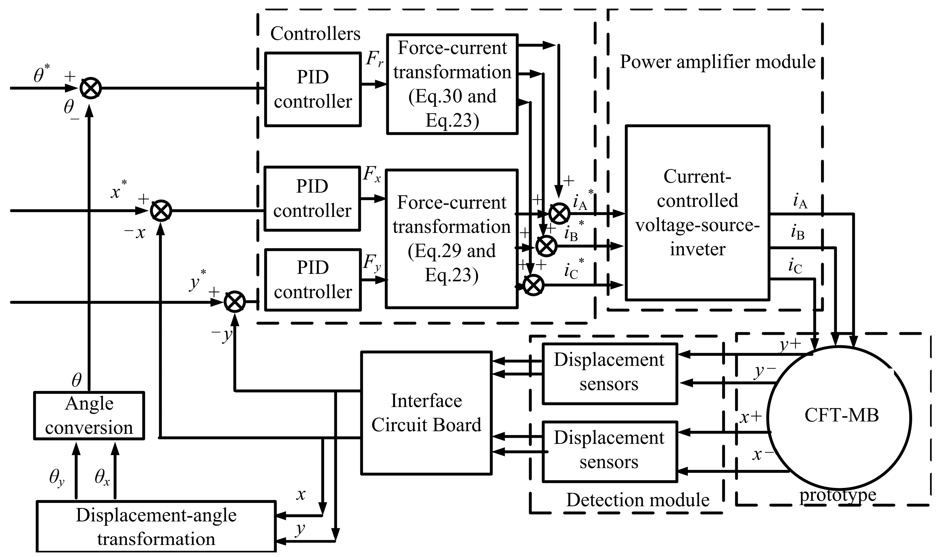
4. Control System Design for a Flywheel Battery Supported with Spherical Radial AC HMB

Based on the established model above, the control system of spherical radial AC HMB is designed, which mainly includes the vertical test bench, hardware system and software system, as shown in Figure 7 and Figure 8. It is worth noting that five displacement sensors (eddy current displacement sensors) are used in our control system. Among them, four radial sensors are the main ones, and the axial sensor is the auxiliary one. In order to realize differential detection, the radial sensors installed symmetrically for each degree of freedom are located. In addition, the installation of the axial sensor can quickly detect whether radial eccentricity occurs to the rotor. Since one side of the rotor is fixed, this axis is similar to an inverted pendulum. Once radial eccentricity occurs, the axial sensor must perceive it. Therefore, the rotor eccentricity can be quickly and roughly judged from the detection data of the axial sensor. Of course, the radial sensors with differential installation are the main sensors responsible for the specific eccentric distances of the rotor.

What is more, from Figure 7, it can be seen that the vertical test bench is designed to simulate the magnetic suspension support system of the flywheel battery, thus it is not a real flywheel system. The spherical radial AC HMB is installed in this vertical test bench to verify its relative performance. The structure and electricity parameters of the magnetic bearing are shown in

Table 1. Prototype parameter results.

Item	Value	Item	Value
Spherical air gap length δ0 (mm)	0.5	Axial length of permanent magnet (mm)	6
Radius of auxiliary bearing (mm)	0.25	Inner diameter of permanent magnet (mm)	106
Number of turns of windings	350	Outside diameter of outer aluminum ring (mm)	132
Wire diameter of control windings (mm)	0.45	Inside diameter of outer aluminum ring (mm)	126
Maximum outer diameter of stator (mm)	126	Axial length of outer aluminum ring (mm)	6

. As shown in Figure 7, in the vertical test bench, the two-section shaft is joined together by a universal joint. The shaft at the upper end of the universal joint is suspended by a radial magnetic bearing and is protected by two mechanical auxiliary bearings. The shaft at the lower end of the universal joint is driven and rotated by a motor. Because of the displacement constraint of the cardan axis on the rotor on the z axis, the controlled suspension rotor has two degrees of freedom (x and y in the radial direction). Therefore, the device can be equivalent to the gyroscope (fixed point motion of rigid body), and the gyroscopic effect of a maglev rotor system under the influence of vehicle conditions can be well tested by this method. In addition, because the device is similar to an inverted pendulum system, displacement eccentricity and deflection motion are virtually the same motion for the position sensors. Therefore, the control system adopts a position and angle double closed-loop control, which improves the real-time performance and stability of the system.

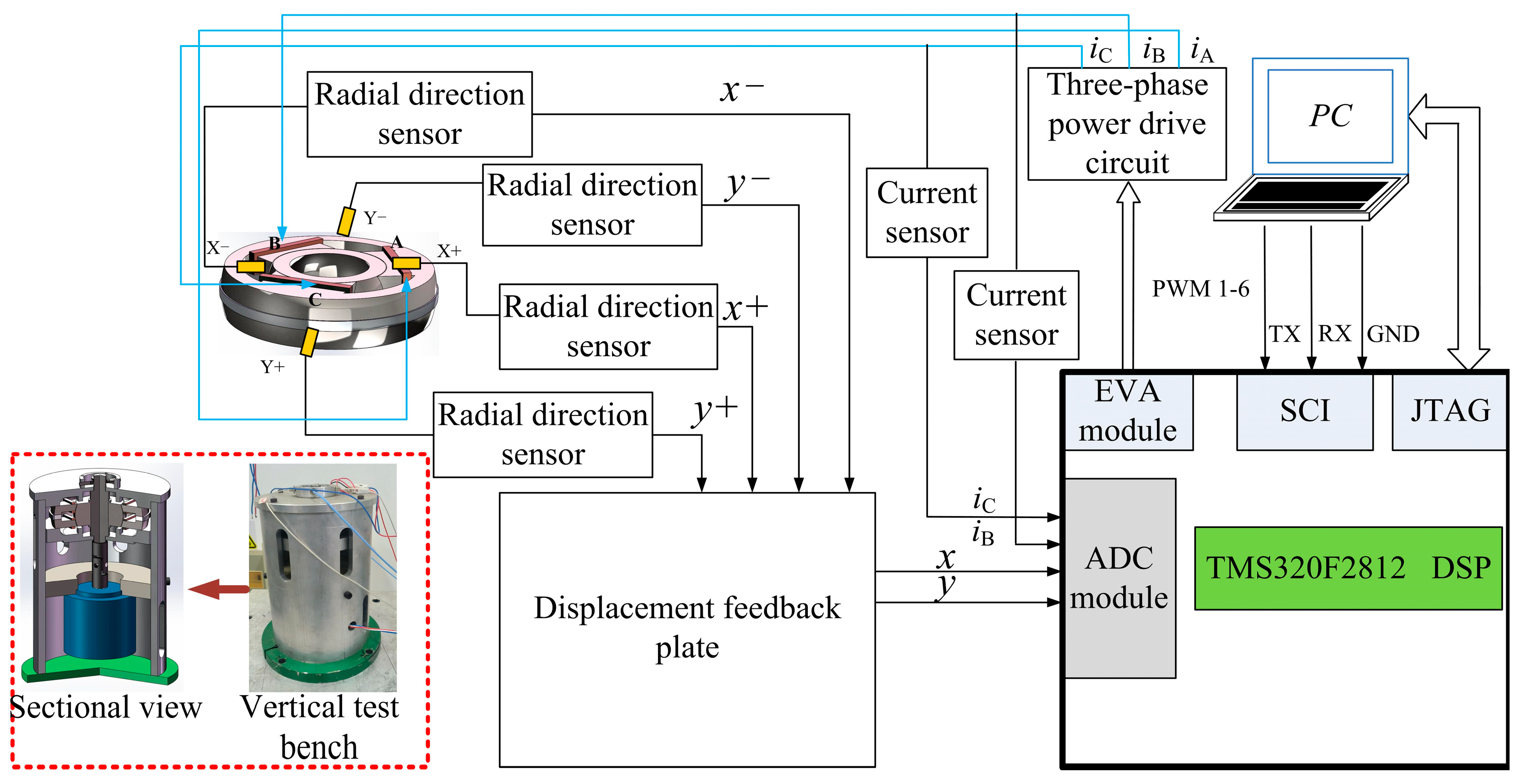
4.1. Digital Control System Hardware Design

(1)

TMS320F2812DSP control board

TMS320F2812DSP is used as the core controller of the whole control system. A DSP control board based on this chip is designed. The digital control system composed of the main control board can meet the design requirements of stable flywheel battery operation. Because the operating voltage and current of the circuit board of the control board and other functional modules are different, it is necessary to design the corresponding interface circuit. Interface circuits are mainly divided into two categories: one is the displacement interface conversion circuit, the other is the output interface conversion circuit.

(2)

Displacement feedback plate

Radial displacement feedback circuit (x, y axis): four eddy current sensors are installed along the radial direction to generate radial displacement signals. Differential processing of signals can eliminate the mechanical coupling effect caused by the asymmetric arrangement of three-phase system. In this design, the displacement detection circuit in the x direction is the same as that in the y direction. First, the sensor input is used to collect the signal. The input displacement signal is processed by voltage regulation and frequency division to realize voltage following. Then the displacement deviation in this direction is calculated by the difference of two displacement data. The sensor input displacement signal voltage is −2 ~ 18V, and the final output displacement signal is 0 ~ 3.3V. This is because the controller digital sampling module working range is 0 ~ 3.3V. Therefore, it is necessary to process the input signal and stabilize the final output at 1.65–2.65V by pulling up the power supply at 1.65V. This design can improve the sensitivity of displacement feedback data and filter out noise interference during sensor sampling.

(3)

Driving board

(a) Radial three-phase power supply driving circuit: three IRS2106SPBF drives three-phase output, respectively, to improve output capacity. At the same time, the output of each phase is protected to ensure that the MOSFET can be turned off quickly when the reversing voltage is needed and improve the switching frequency. Twelve power transistors work together to regulate the output of the driving voltage. According to the rotor displacement feedback, the processor gives the corresponding ACTRA value, and changes the size and direction of the control current by changing the duty ratio of the three-phase PWM signal. Finally, the rotor is suspended in radial stability.

(b) Current sensor: According to the design, the maximum current of the control coil is ±1A. Therefore, the current sampling value is between −1A and 1A, and the output voltage after passing through the current sensor is 1.581V to 1.719V. The voltage signal output to the processor ranges from 0V to 3.3V. The current feedback value is compared to the current value calculated by the processor, and the output current is adjusted. The design can stabilize the output current and prevent current mutation from damaging the system.

(4)

Power output board

The function of this circuit is to amplify the radial three-phase output power. Generally, the structure of a three-phase full-bridge inverter is adopted. Each circuit phase consists of three electric field-effect transistors in parallel to form a switch. In this way, the large current can be switched on and off to ensure repeated space for future upgrades. Through the processor output PWM wave control radial, three-phase drive circuits of 12 power transistors on and off. By adjusting the duty ratio of the PWM wave, you can adjust the output voltage and then adjust the 18 electric field-effect transistors on the three-phase bridge on and off. Finally, the size and direction of the control current in the radial magnetic bearing current coil can be adjusted. The switching frequency and stability of system output can be improved by this design.

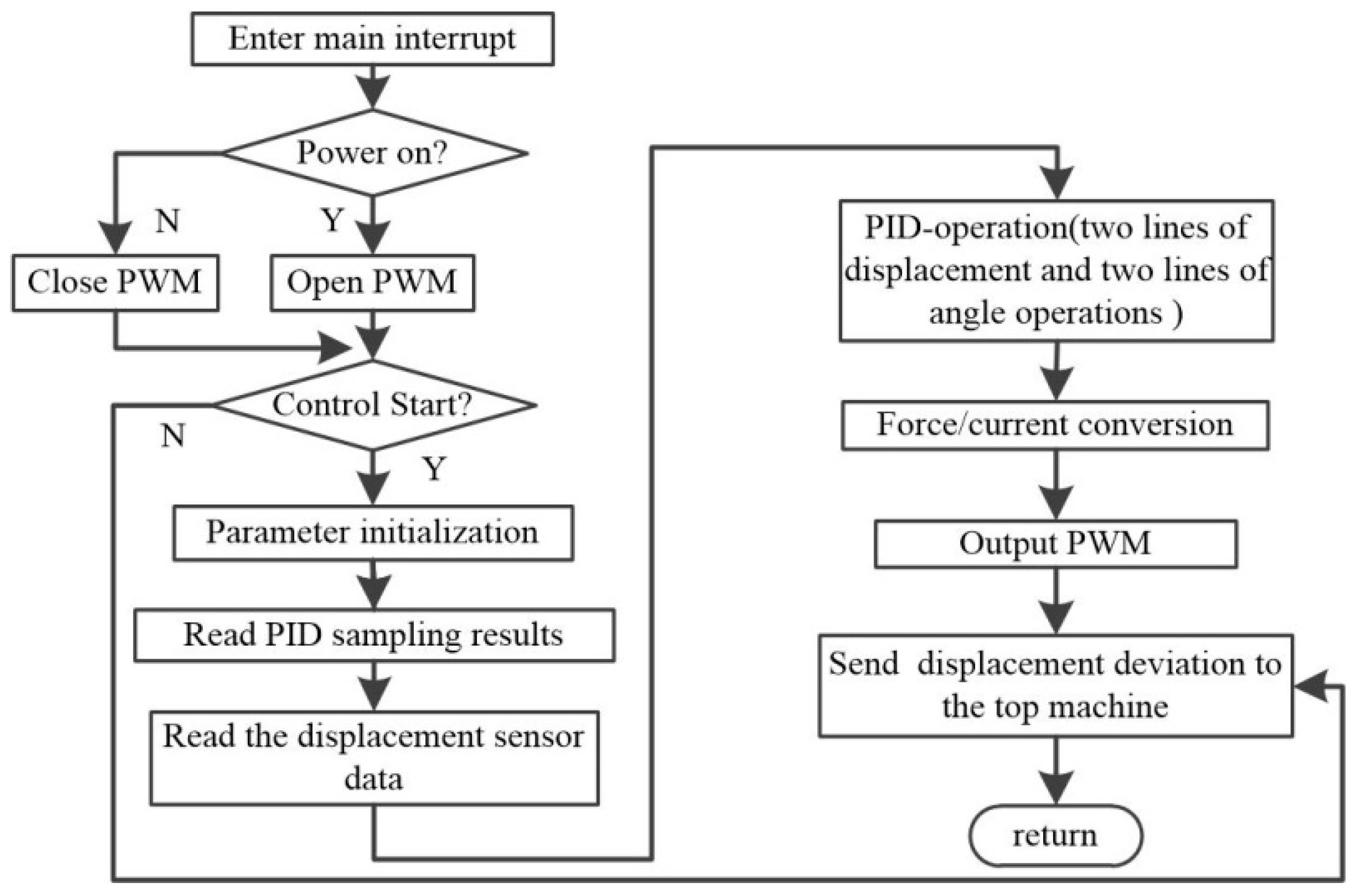
4.2. Control System Software Programming

The software algorithm of the control system is described in Figure 8. It is worth noting that in order to improve the control accuracy, the relationship between the force and deflection angle as a model are added into the control system, therefore, the dual control of displacement and angle can be realized. In Figure 8, the force-current conversion link reflects the mathematical model of suspension force (Equations (29) and (30)). When the rotor deviates from the equilibrium position due to the disturbance, the position sensor measures the offset value of the rotor and transmits the displacement signal to the controller through the interface circuit board. When the rotor is disturbed and deflects, two angle signals can be obtained by the displacement-angle conversion module. Then, an angle signal after the angle conversion signal is derived and transmitted to the controller. A compound motion can even contain two motions at the same time. The controller converts the displacement and deflection angle signals into control current signals. The three-phase inverter is driven by the control signal and outputs the excitation current. It is worth noting that the non-existent angle sensor is implemented by displacement sensors and some processing circuits. Since the axis is a fixed point motion, the angle of deflection can be easily measured.

As shown in Figure 9, the software of the control system is composed of the main program and an interrupt service subroutine module. The main program mainly completes the initialization of the system clock and EV, SCI, ADC and other functional modules. The main program then starts the timer, enters the interrupt loop, and waits for the interrupt. The interrupt service program consists of three main parts: the main interrupt service program, the receiving interrupt service program and the sending interrupt service program. The main interrupt service subroutine is the radial magnetic bearing control part. Through the comparison unit in DSP event manager A module, a 6-channel pulse width modulation (PWM) wave (PWM1-6) can be generated to complete the data sampling processing and control algorithm implementation. The detailed procedure is as follows: First, the receiving interrupt receives the signal sent by the upper computer. The main process of interrupt service includes ADC sampling data collection, PID data calculation and PWM output selection. The last interrupt sends the ADC sampling value to the upper computer, which can visually display the rotor displacement value in time. The receive interrupt service program is used to receive PID parameters and easily modify them in time through the user interface.

LabVIEW programming language was used to write the upper computer interface program. The received displacement data are processed and displayed in the waveform diagram. This gives a clear picture of the displacement. The received current data are processed and displayed with a pointer meter to give a clear picture of the current range.

To keep the program simple and straightforward, each function program is designed as a subvi, which is encapsulated and can be called directly as a function. The main function modules are power switch, input confirmation, sending data, receiving data and so on. The program structure mainly adopts event structure and condition structure. Event structure and condition structure are similar to interrupt structure in program, as long as the corresponding event is triggered, the corresponding setting operation will be carried out. It is important to note that event structures and conditional structures have the same priority. It is necessary to set an appropriate timeout, otherwise the program will not work properly. Not paying attention to this at first can lead to crashes and confusion. The communication adopts SCI communication, and the VISA function module of LabVIEW completes the data sending and receiving function.

The main steps of the control interface program are as follows: First, input PID parameters to check whether the parameters are within a reasonable range. Then, turn on the power switch and send the data to the DSP. Receive the feedback data of the lower machine for display and observation processing.

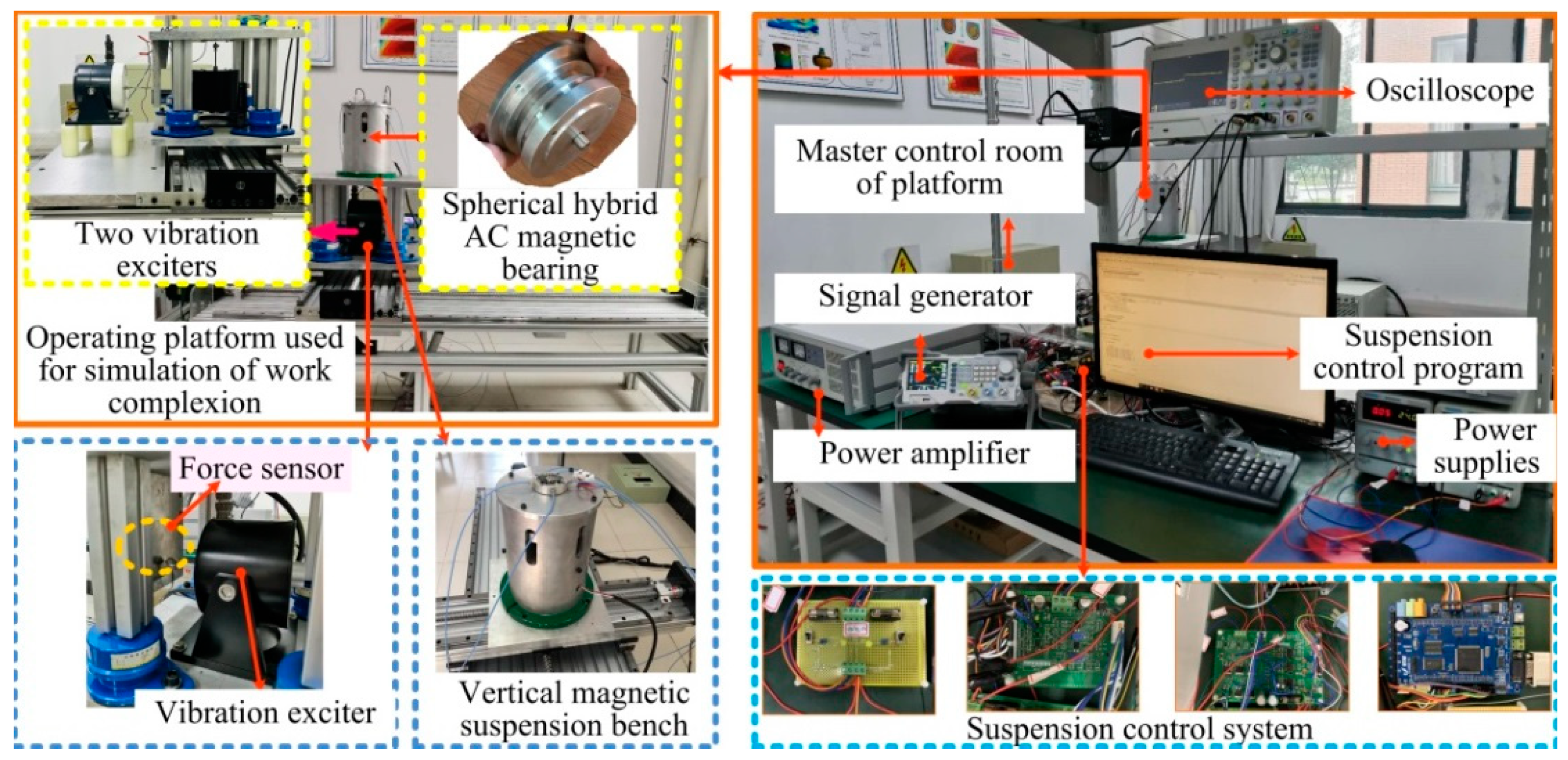
5. Experiment and Analysis

The experimental platform is illustrated in Figure 10. It is based on the hardware block diagram presented in Figure 7 and the physical map of each module of the control system presented in Figure 8. Various testing experiments and various advanced control algorithms can be verified in this experimental platform. This overall platform mainly includes a vertical magnetic suspension bench, an operating platform for imitating automobile suspension, driving conditions and road conditions, and a suspension control system controller. The spherical radial AC HMB prototype is installed inside the vertical magnetic suspension bench which is used to simulate the actual vertical magnetic suspension flywheel battery. The automobile suspension system is imitated by four spring shock absorbers while road conditions are imitated by a function signal generator and vibration exciters. The vibration exciters are used to imitate the driving conditions. The position and number of vibration exciters can be adjusted at any time according to the experimental requirements of vehicle conditions. In addition, road functions can be programmed by the signal generator to drive the right vibration exciter to imitate a road. Further, the strength of the interference signal is judged by a force sensor. What is more, the excitation force signal is output by the force sensor at the pole, and the actual acceleration value can be simulated according to the relationship between force, mass and acceleration under the condition of knowing the overall mass of the excited object.

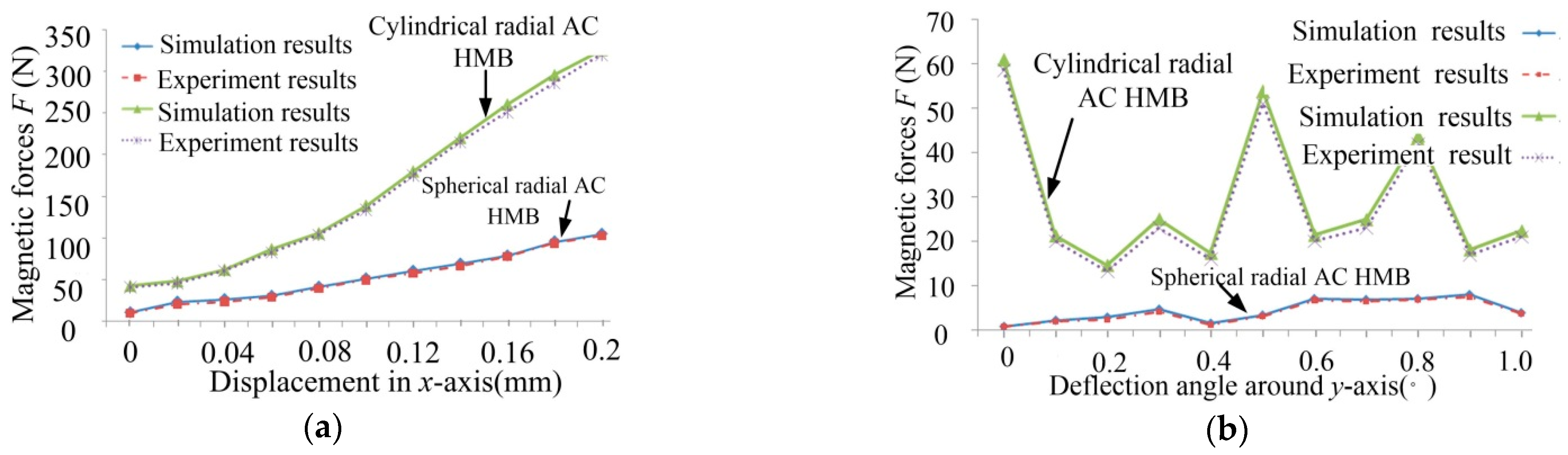
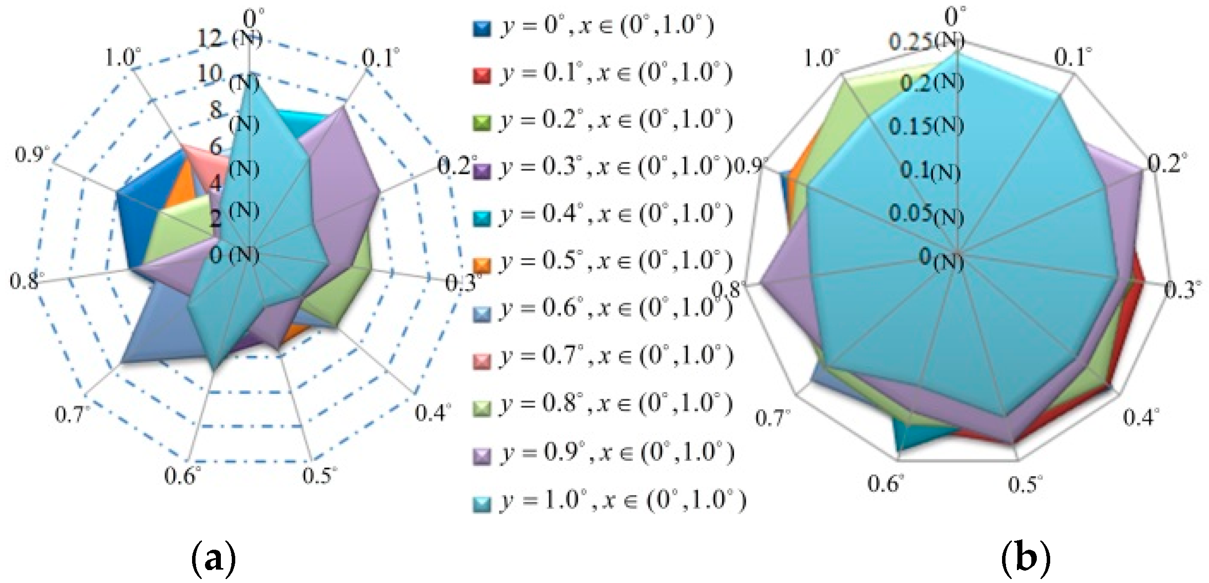
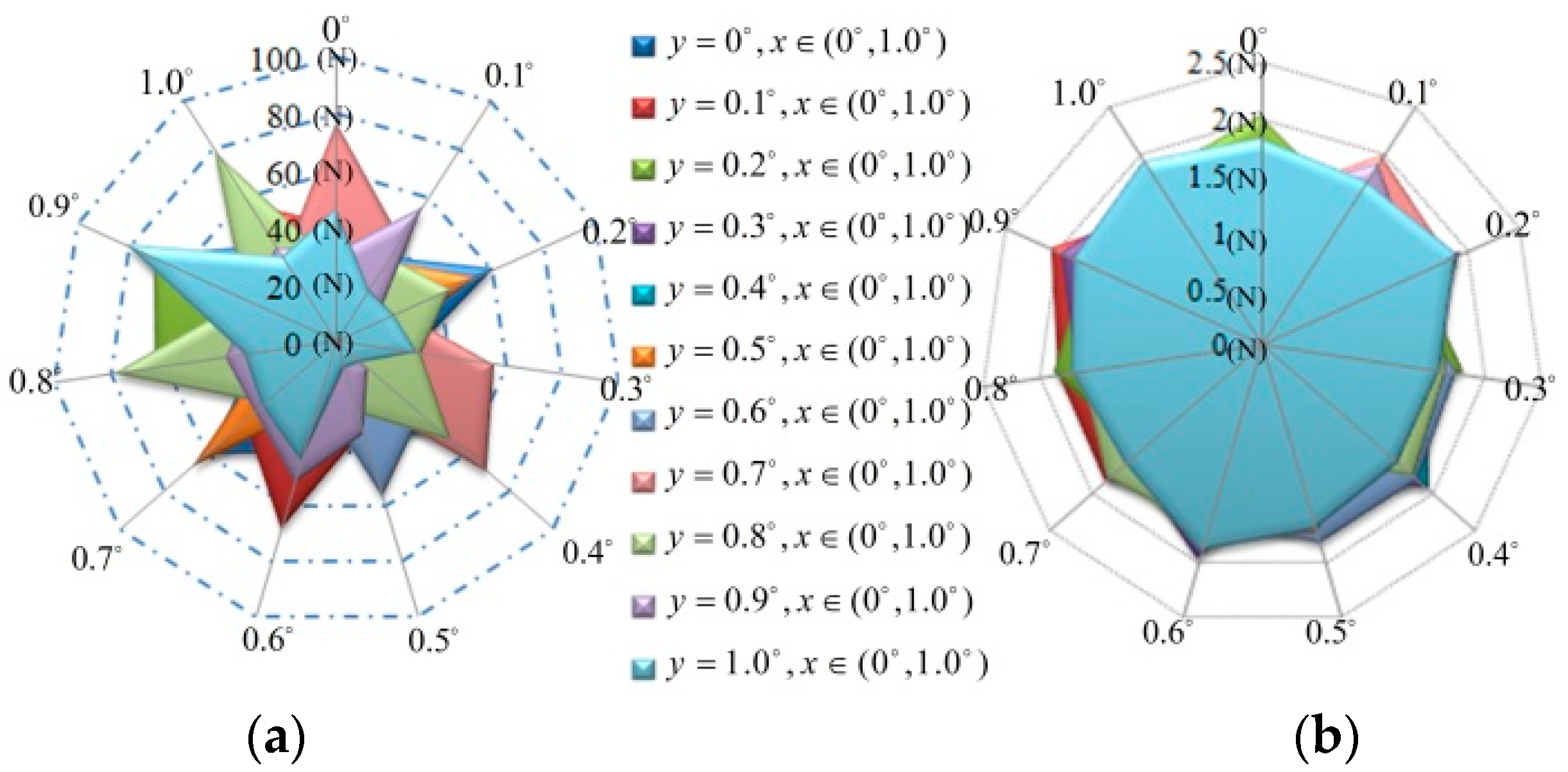
5.1. Stiffness Tests

Stiffness tests are conducted to prove the accuracy and universality of the model. To prove the accuracy and universality of the modeling method, the spherical radial AC HMB and radial AC HMB are both used to test and compare based on the same experimental platform. Figure 11a shows the relation curve between the displacement x on the x axis and the resultant suspension force F when the rotor moves 0.2mm on the y axis. Figure 11b shows the relation curve between the rotor deflection angle around the y axis and the resultant suspension force F when the rotor is deflected 0.2° around the x axis. It can be seen from Figure 11 that for the two magnetic bearings the stiffness curves (force-displacement and force-deflection coefficients) of the calculated results are close to those of the test results, which can verify the accuracy and universality of the modeling method.

In order to further prove the universality and accuracy of the model, full force-deflection stiffness tests are conducted. Figure 12 shows the experimental results of the suspension force around the x axis and y axis as a function of the deflection angle. In this experiment, the angle about the x axis varies between 0° and 1.0°, and the angle about the y axis varies between 0° and 1.0°. The relationship between the resultant amplitude and the deflection angle of the two axes can be obtained by using the polar surface with full stiffness, as shown in Figure 12a. The relative error between the calculated value and the experimental value is shown in Figure 12b. In contrast, as shown in Figure 13, suspension forces and deflection angles around the x and y axes of the cylindrical magnetic bearing are also tested. The error between the improved model and the force-deflection stiffness test results is within 2.8%. It can be seen from Figure 12 and Figure 13 that the improved Maxwell tensor modeling method has good universality and can ensure the accuracy of the suspension force modeling of spherical and cylindrical magnetic bearings.

5.2. Performance Tests

The performance tests under the two most typical vehicle operation conditions were conducted. It is worth noting that in order to highlight the influence of the vehicle driving on the stability of the flywheel battery system, the influence of the gyroscopic effect generated by the high-speed flywheel is excluded. Therefore, the rotor speed was not set very high when doing the vehicle driving condition experiment. The running speed of the rotor was set to 1100 r/min.

(1)

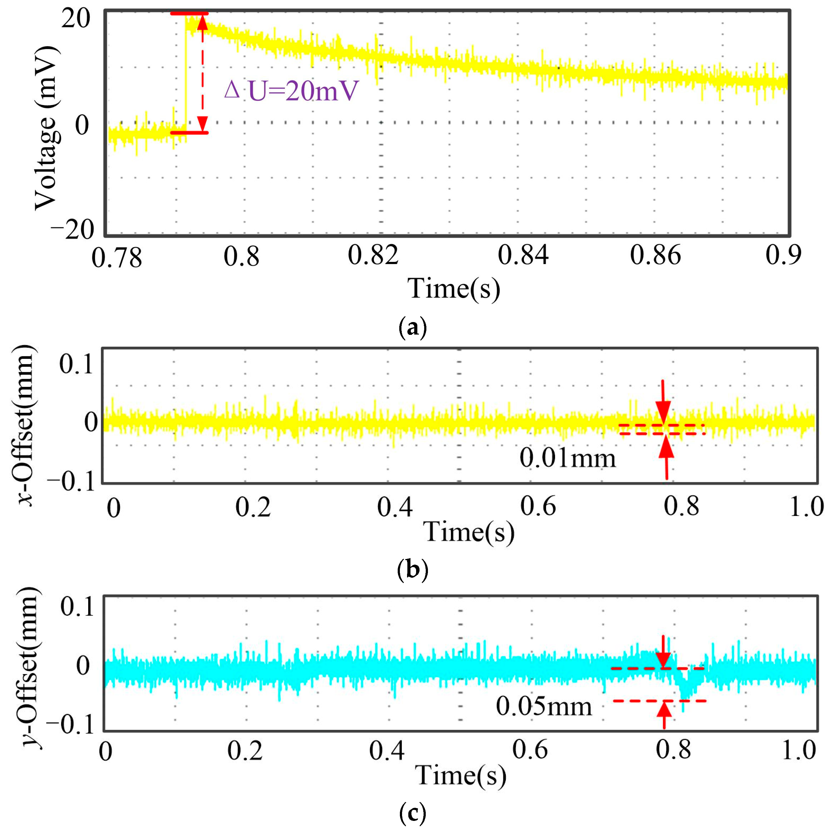
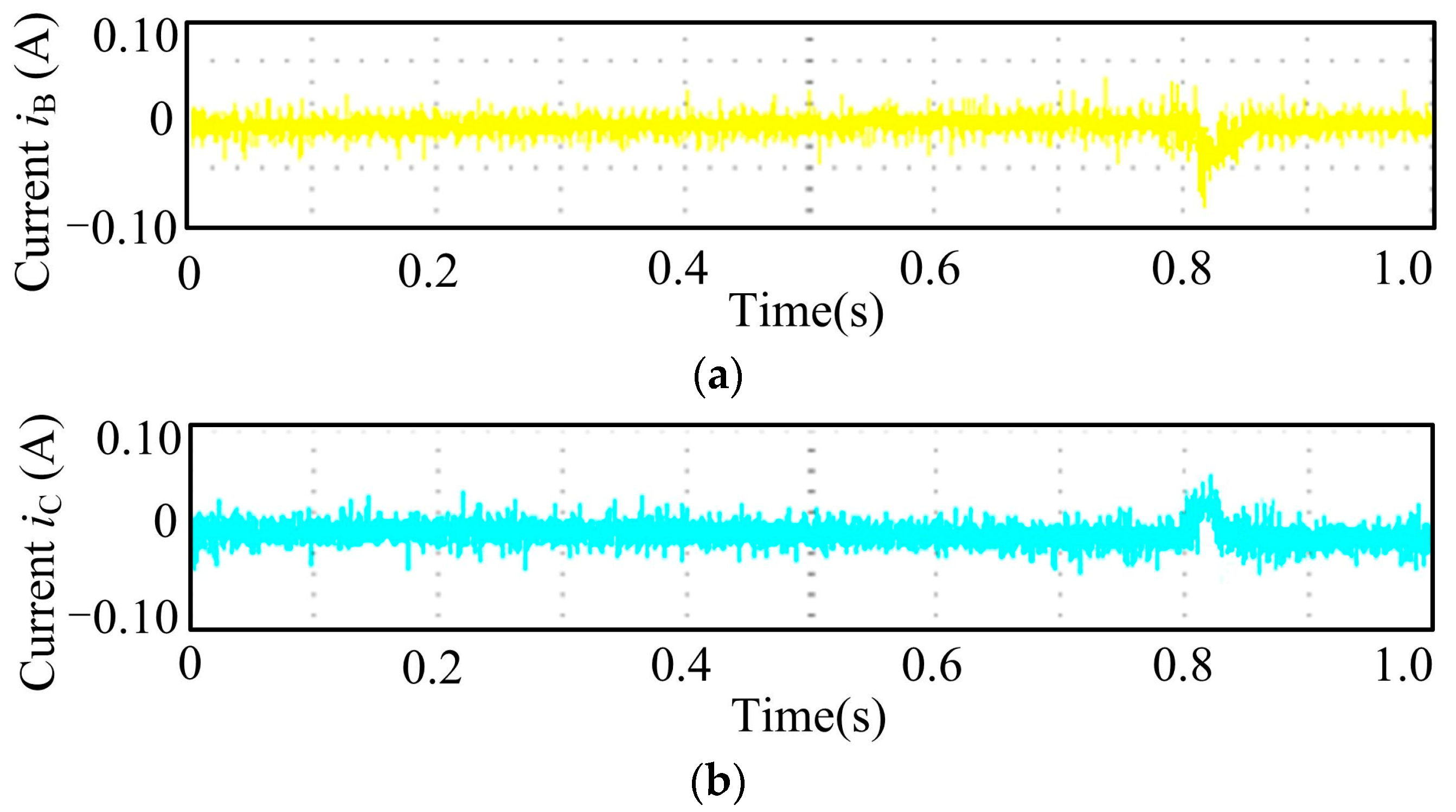
Acceleration disturbance experiment

Based on the experimental platform in Figure 10, the experimental tests have been done to simulate the acceleration of a vehicle. In this test, the frequency of excitation signal was set to 1Hz, which is convenient to observe the force signal during the sudden impact. As shown in Figure 14a, the output waveform of the force signal at a certain moment can be seen. At this time, the excitation direction of the vibration exciter was a radial y direction. According to the relationship between the force and voltage of the force sensor (0–5 V corresponds to 0–5000 N), the output force at that moment was about 20 N, so it can be deduced that the acceleration at that time was about 2m/s². Figure 14b,c show the results of rotor displacement deviation under the condition of 2m/s² acceleration in x and y directions. From Figure 14b, it can be seen that the maximum offset of the rotor in x direction was 0.01 mm and the adjustment time was approximately 8 ms. At the same time, Figure 14c shows the offsets in the y direction was 0.05 mm and the adjustment time was approximately 30 ms. Experimental results show that, under the control system, the rotor can return to the equilibrium position in a short time, although the rotor will produce some eccentricity under the disturbance caused by vehicle acceleration. Furthermore, the results show that the acceleration acting in the y direction does not have great influence on the x direction.

What is more, the corresponding current waveforms of the disturbed rotor in the accelerated experiment are shown in Figure 15a,b, respectively. Since the real-time sum of the three-phase control current is zero, the third current phase can be calculated as long as any two-phase current is known. Therefore, just the two phase currents (B- and C-phase control currents) that are often measured in daily experiments are given below. From Figure 14 and Figure 15, it can be seen that under the regulation of a control current, once the disturbance disappears, the rotor quickly returns to the equilibrium position, and the changed current can be quickly restored to the original zero value.

(2)

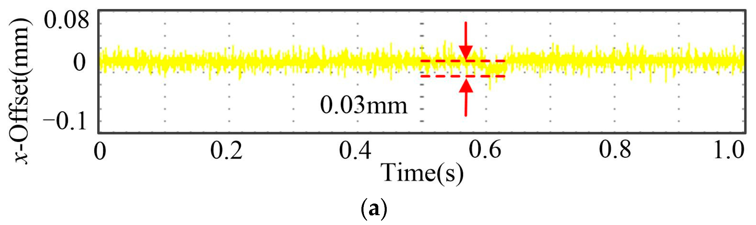
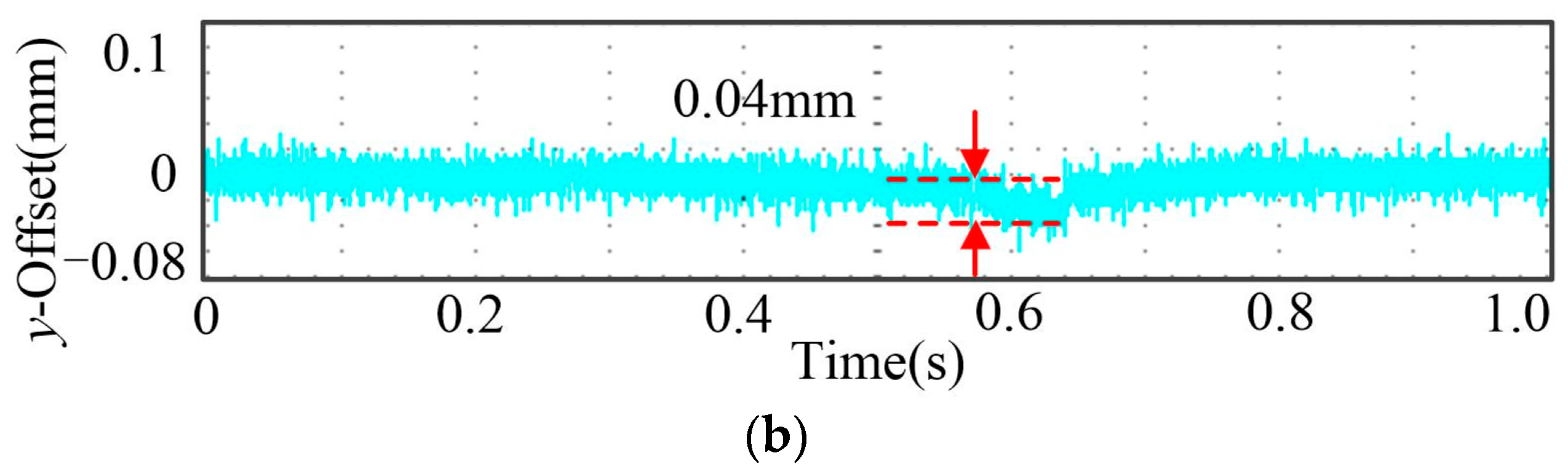
Turning disturbance experiment

Based on the experimental platform in Figure 10, the experimental tests have been done to simulate the turning of a vehicle. In this test, the disturbance was applying a force of 20N at some point in time in both the x and y directions. According to the relationship between force and voltage of the force sensor (0–5 V corresponds to 0–5000 N), the output force at this moment was about 20 N, so the acceleration at that time was also about 2 m/s². It is worth noting that in this test, the frequency of excitation signal was also set to 1 Hz, which is convenient to observe the force signal during the sudden impact. Different from the previous acceleration condition, this experiment required two vibration exciters to stimulate in the x and y directions at the same time. Since this experiment was also conducted with the acceleration of 2 in the x and y directions, and the force of the vibration exciter under the same voltage was exactly the same, the force signal diagram of the output of the vibration exciter is not repeated here.

It can be seen from Figure 16a that the maximum offset of the rotor in the x direction was 0.03 mm and the adjustment time was about 8 ms. Meanwhile, Figure 16b shows the maximum offset of the rotor in the y direction was 0.04 mm and the adjustment time was about 8 ms. The experimental results show that the rotor can return to the equilibrium position in a short time under the action of the control system, although some eccentricity of the rotor is generated under the disturbance caused by vehicle turning. At the same time, it can also be observed from the test waveform that since the acceleration excitation of the same magnitude was in the x and y directions at the same time, the responses in the two degrees of freedom directions are also very similar.

The control current waveforms corresponding to the rotor displacement waveforms in the turning experiment are shown in Figure 17. Similarly, only two phase currents (B- and C-phase control currents) are measured. From Figure 16 and Figure 17, it can be seen that under the regulation of the control current, once the disturbance disappears, the rotor quickly returns to the equilibrium position, and the changed current can also be quickly restored to the original zero value.

6. Conclusions

In this study, an accurate mathematical model of suspension forces for a spherical radial AC HMB adopting wide-area and universal modeling theories for a magnetic suspension flywheel battery is deduced in detail. Then, the accuracy, wide-area and universality analyses are conducted. Further, based on the established model, the control system is designed, which includes the overall schematic, hardware, and software designs. Finally, relevant comparative tests are conducted to validate the accuracy and universality of the established model. The good stiffness test results show that, compared with the equivalent magnetic circuit method, the improved Maxwell tensor method can make the modeling result more accurate. In addition, the consistent comparison results of the full stiffness tests show that the proposed modeling method has good universality. The good test results of the disturbance performance caused by vehicle operating conditions prove the effectiveness of the modeling method and control system proposed in this study.

References

1. Sun, B.; Dragičević, T.; Freijedo, F.D.; Vasquez, J.C.; Guerrero, J.M. A control algorithm for electric vehicle fast charging stations equipped with flywheel energy storage systems. IEEE Trans. Power Electron. 2016, 31, 6674–6685. [Google Scholar] [CrossRef] [Green Version]
2. Zhang, W.Y.; Zhu, P.F.; Cheng, L.; Zhu, H.Q. Improved centripetal force type-magnetic bearing with superior stiffness and anti-interference characteristics for flywheel battery system. Int. J. Precis. Eng. Manuf.-Green Technol. 2020, 7, 713–726. [Google Scholar] [CrossRef]
3. Oh, Y.; Kwon, D.-S.; Eun, Y.; Kim, W.; Kim, M.-O.; Ko, H.-J.; Kang, S.G.; Kim, J. Flexible energy harvester with piezoelectric and thermoelectric hybrid mechanisms for sustainable harvesting. Int. J. Precis. Eng. Manuf.-Green Technol. 2019, 6, 691–698. [Google Scholar] [CrossRef]
4. Zhang, W.Y.; Gu, X.W.; Zhang, L.D. Robust controller considering road disturbances for a vehicular flywheel battery system. Energies 2022, 15, 5432. [Google Scholar] [CrossRef]
5. Park, H. Vibratory electromagnetic induction energy harvester on wheel surface of mobile sources. Int. J. Precis. Eng. Manuf.-Green Technol. 2017, 4, 59–66. [Google Scholar] [CrossRef]
6. Zheng, S.Q.; Yang, J.Y.; Song, X.D.; Ma, C. Tracking compensation control for nutation mode of high-speed rotors with strong gyroscopic effects. IEEE Trans. Ind. Electron. 2018, 65, 4156–4165. [Google Scholar] [CrossRef]
7. Li, X.J.; Anvari, B.; Palazzolo, A.; Wang, Z.Y.; Toliyat, H. A utility-scale flywheel energy storage system with a shaftless, hubless, high-strength steel rotor. IEEE Trans. Ind. Electron. 2018, 65, 6667–6675. [Google Scholar] [CrossRef]
8. Ren, Y.; Chen, X.C.; Cai, Y.W.; Zhang, H.J.; Xin, C.J.; Liu, Q. Attitude-rate measurement and control integration using magnetically suspended control and sensitive gyroscopes. IEEE Trans. Ind. Electron. 2018, 65, 4921–4932. [Google Scholar] [CrossRef]
9. Lyu, X.; Di, L.; Yoon, S.Y.; Lin, Z.; Hu, Y. A platform for analysis and control design: Emulation of energy storage flywheels on a rotor-AMB test rig. Mechatronics 2016, 33, 146–160. [Google Scholar] [CrossRef]
10. Matsuzaki, T.; Takemoto, M.; Ogasawara, S.; Ota, S.; Oi, K.; Matsuhashi, D. Novel structure of three-axis active-control-type magnetic bearing for reducing rotor iron loss. IEEE Trans. Magn. 2016, 52, 81054043. [Google Scholar] [CrossRef]
11. Han, B.C.; Xu, Q.J.; Yuan, Q. Multiobjective optimization of a Combined radial-axial magnetic bearing for magnetically suspended compressor. IEEE Trans. Ind. Electron. 2016, 63, 2284–2293. [Google Scholar]
12. Ravaud, R.; Lemarquand, G.; Lemarquand, V. Force and stiffness of passive magnetic bearing using permanent magnets. Part 1: Axial magnetization. IEEE Trans. Magn. 2009, 45, 2996–3002. [Google Scholar] [CrossRef] [Green Version]
13. Sun, J.J.; Ju, Z.Y.; Peng, C. A novel 4-DOF hybrid magnetic bearing for DGMSCMG. IEEE Trans. Ind. Electron. 2017, 64, 2196–2204. [Google Scholar] [CrossRef]
14. Zhang, W.Y.; Zhu, H.Q. Control system design for a five-degree-of-freedom electrospindle supported with AC hybrid magnetic bearings. IEEE/ASME Trans. Mechatron. 2015, 20, 2525–2537. [Google Scholar] [CrossRef]
15. Zhang, W.Y.; Wang, J.P.; Zhu, P.F. Design and analysis of a centripetal force type-magnetic bearing for a flywheel battery system. Rev. Sci. Instrum. 2018, 89, 064708. [Google Scholar] [CrossRef]
16. Mushi, S.E.; Lin, Z.L.; Allaire, P.E. Design construction and modeling of a flexible rotor active magnetic bearing test rig. IEEE/ASME Trans. Mechatron. 2012, 17, 1170–1182. [Google Scholar] [CrossRef]
17. Zad, H.S.; Khan, T.I.; Lazoglu, I. Design and adaptive sliding-mode control of hybrid magnetic bearings. IEEE Trans. Ind. Electron. 2018, 65, 2449–2457. [Google Scholar]
18. Soni, T.; Dutt, J.K.; Das, A.S. Parametric stability analysis of active magnetic bearing-supported rotor system with a novel control law subject to periodic base motion. IEEE Trans. Ind. Electron. 2020, 67, 1160–1170. [Google Scholar] [CrossRef]
19. Park, S.-H.; Lee, C.-W. Decoupled control of a disk-type rotor equipped with a three-pole hybrid magnetic bearing. IEEE Trans. Ind. Electron. 2010, 15, 793–804. [Google Scholar]
20. Zhang, W.; Zhu, H.; Yang, Z.; Sun, X.; Yuan, Y. Nonlinear model analysis and “switching model” of AC-DC three-degree of freedom hybrid magnetic bearing. IEEE/ASME Trans. Mechatron. 2016, 21, 1102–1115. [Google Scholar] [CrossRef]
21. Tang, J.Q.; Wang, K.; Xiang, B. Stable control of high-speed rotor suspended by superconducting magnetic bearings and active magnetic bearings. IEEE Trans. Ind. Electron. 2017, 64, 3319–3328. [Google Scholar] [CrossRef]
22. Zhang, W.Y.; Yang, H.K.; Cheng, L.; Zhu, H.Q. Modeling based on exact segmentation of magnetic field for a centripetal force type-magnetic bearing. IEEE Trans. Ind. Electron. 2020, 67, 7691–7701. [Google Scholar] [CrossRef]
23. Zhang, W.Y.; Cheng, L.; Zhu, H.Q. Suspension force error source analysis and multidimensional dynamic model for a centripetal force type-magnetic bearing. IEEE Trans. Ind. Electron. 2020, 67, 7617–7628. [Google Scholar] [CrossRef]
24. Zhang, W.Y.; Zhu, H.Q. Precision modeling method specifically for AC magnetic bearings. IEEE Trans. Magn. 2013, 49, 5543–5553. [Google Scholar] [CrossRef]
Figure 1. Structure and magnetic circuits of spherical radial AC HMB (a) Assembling structure and exploded view. (b) Sketch of the magnetic circuits.
Energies 16 01973 g001
Figure 2. Coordinate system and rotor eccentricity diagram.
Energies 16 01973 g002
Figure 3. Calculation of geometric angle of stator.
Energies 16 01973 g003
Figure 4. Permanent magnet.
Energies 16 01973 g004
Figure 5. Calculation of geometric angle of rotor.
Energies 16 01973 g005
Figure 6. Coordinate systems and rotor deflection diagrams.
Energies 16 01973 g006
Figure 7. Hardware block diagram.
Energies 16 01973 g007
Figure 8. Suspension control diagram.
Energies 16 01973 g008
Figure 9. Program flow chart.
Energies 16 01973 g009
Figure 10. Experimental platform.
Energies 16 01973 g010
Figure 11. Stiffness comparison diagram. (a) Comparison of modeling results of force–displacement stiffness with experimental results. (b) Comparison of modeling results of force–deflection stiffness with experimental results.
Energies 16 01973 g011
Figure 12. Full stiffness of spherical radial AC HMB (suspension forces versus deflection). (a) Experimental value. (b) Relative error between calculated value and experimental value.
Energies 16 01973 g012
Figure 13. Full stiffness of cylindrical magnetic bearing (suspension forces versus deflection). (a) Experimental value. (b) Relative error between calculated value and experimental value.
Energies 16 01973 g013
Figure 14. Experimental results in accelerated experiment. (a) The force signal output by vibration exciter. (b) Rotor offset in x direction. (c) Rotor offset in y direction.
Energies 16 01973 g014
Figure 15. Control current waveforms in accelerated experiment. (a) B-phase control current iB. (b) C-phase control current iC.
Energies 16 01973 g015
Figure 16. Experimental results in turning experiment. (a) Rotor offset in x direction. (b) Rotor offset in y direction.
Energies 16 01973 g016aEnergies 16 01973 g016b
Figure 17. Control current waveforms in turning experiment. (a) B-phase control current iB. (b) C-phase control current iC.
Energies 16 01973 g017