An Adaptive, Data-Driven Stacking Ensemble Learning Framework for the Short-Term Forecasting of Renewable Energy Generation

Abstract

With the increasing integration of wind and photovoltaic power, the security and stability of the power system operations are greatly influenced by the intermittency and fluctuation of these renewable sources of energy generation. The accurate and reliable short-term forecasting of renewable energy generation can effectively reduce the impacts of uncertainty on the power system. In this paper, we propose an adaptive, data-driven stacking ensemble learning framework for the short-term output power forecasting of renewable energy. Five base-models are adaptively selected via the determination coefficient (R²) indices from twelve candidate models. Then, cross-validation is used to increase the data diversity, and Bayesian optimization is used to tune hyperparameters. Finally, base modes with different weights determined by minimizing the cross-validation error are ensembled using a linear model. Four datasets in different seasons from wind farms and photovoltaic power stations are used to verify the proposed model. The results illustrate that the proposed stacking ensemble learning model for renewable energy power forecasting can adapt to dynamic changes in data and has better prediction precision and a stronger generalization performance compared to the benchmark models.

1. Introduction

With increasing global climatic warming and environmental issues, renewable energy sources are receiving increasing attention, especially wind and solar power. Due to the randomness and intermittency of wind and solar resources, the high penetration of wind and photovoltaic (PV) power generation causes uncertainty in the power system. Accurate and stable short-term forecasting for wind and PV output power is crucial to maintain the balance between the supply and demand of power systems, optimize the configuration of rotating reserve capacity, and make dispatching decisions in the power market environment [1,2]. Data-driven prediction models for wind and solar renewable energy combined with artificial intelligence and machine learning technology are widely used, owing to their strong ability to mine historical data [3].

For data-driven renewable energy generation prediction, a complex nonlinear mapping relationship between the input features and the output power usually needs to be constructed. Traditional time series models such as regressive (AR), AR moving average (ARMA), and AR integrative moving average only define a linear mapping relationship between input and output, increasing the prediction error with each forecast interval [4]. Advanced machine learning methods are capable of building a strong nonlinear input–output map through a black-box concept [5,6]. A number of regression models use black- box mapping, e.g., artificial neural network (ANN) [7], and support vector machine regression (SVR) [8]. ANNs simulate the biological neural network constituting the brain, consisting of a number of connected neurons that carry and transmit signals. Deep neural network methods, such as autoregressive neural networks [9], convolutional neural networks [10], and long- and short-term memory neural networks [11,12], have been developed rapidly due to their strong feature-capturing ability with little prior knowledge. Nevertheless, the network framework of deep learning is relatively complex, requiring a large amount of training data, and cannot outperform other prediction models with a small sample. SVR uses a kernel function to transform the original feature space to a high-dimensional space, then constructs a linear map, overcoming the problem of dimensionality and achieving effective results with a small sample dataset. Therefore, SVR is selected as the candidate model in this paper.

In recent years, tree ensemble machine learning models [13,14], such as extreme gradient boosting [15] and gradient boosting trees [16], have received increasing attention in industry and academic research due to their open architecture, low computing cost, and robustness. The authors of [17] compared the performance of random forest (RF), extreme regression tree (ET) and support vector machine regression (SVR) for the prediction of photovoltaic power; the ET model achieved the best performance in terms of forecasting accuracy, calculation cost, and stability indices. The authors of [18] described the advantages of tree ensemble learning models, including RF, gradient boosting trees (GBRTs), and extreme gradient boosting (XGB), for wind speed and solar radiation prediction in comparison with the SVR method. The authors of [19] evaluated the performance of XGB and GBRT machine learning methods for solar irradiance prediction. The use of a single model for forecasting renewable energy, as mentioned above, may cause low prediction accuracy and insufficient generalizability when processing various non-stationary datasets.

A hybrid model based on ensemble learning can combine the advantages of different models to improve prediction accuracy and stability performance. Such models are more robust than a single model and are widely applied in energy generation prediction. The authors of [20] proposed a hybrid model combining ET with a deep neural network for the prediction of hourly solar irradiance. The authors of [21] combined a long short-term memory neural network with a convolutional neural network to predict solar irradiance. The authors of [22] adopted a stacking fusion framework based on RF regression tree, adaptive boosting (ADA), and XGB for the prediction of photovoltaic power and achieved improved prediction accuracy. The authors of [23,24] built a new hybrid model based on multiple deep learning methods for wind power prediction. The methods mentioned above use a combined model, improving the prediction accuracy and stability on some levels but ignoring the complex changing dynamic characteristics of the datasets. The factors affecting wind and PV output power are complicated, and the collected meteorological and historical data are high-dimensional and heterogeneous. Therefore, the ensemble learning framework adaptively selects optimal basis models according to data characteristics, representing a key technology to improve the accuracy and generalization performance of prediction models.

In this paper, we propose an adaptive, data-driven stacking ensemble learning framework for predicting renewable energy output power through the deep mining of historical data. Twelve diverse regression models that have been successfully used to mine information hidden in the raw datasets of renewable forecasts are applied as candidate forecast models [25,26,27]. To reduce the negative effects of uncertainty hidden in the historical data and to enhance the generalization performance, an adaptive ensemble framework is developed, which can adaptively select five optimal models based on measurement indices. The optimal hyperparameters of each base-model are tuned using Bayesian optimization, and a linear regression method is employed as a meta-model to combine the five selected base-models. The weight of each base-model can be adaptively obtained according to the principle of cross-validation. Various case studies based on actual data from a wind farm and PV station located in Middle China verify the effectiveness of the proposed adaptive stacking ensemble learning model for renewable energy output power forecasting. In summary, the key contributions of this paper are as follows:

(1)

A novel, data-driven, adaptive stacking ensemble learning framework is developed for the output power forecasting of renewable energy. The stacking structure and different base-models deeply explore the information hidden in the raw data, thereby boosting the regression ability for multi-dimensional heterogeneous datasets.

(2)

Twelve independent candidate regression models, including bagging, boosting, linear, K nearest neighbor and SVR methods, are comprehensively compared. Then, five better models are determined adaptively to integrate the stacking ensemble structure. The diversity among the different base-models can ensure the excellent stability and generalization performance of the stacking model.

(3)

A meta-model is constructed using the linear regression method. The weights of base-models are determined via minimizing the cross-validation risk of the base-models estimator.

(4)

The hyperparameters of base-models and meta-model are tuned and optimized using the Bayesian global optimization method, which further enhances the forecasting accuracy of the proposed model.

2. Adaptive Ensemble Learning Framework for Renewable Energy Forecast

Twelve methods with good performance for renewable energy power prediction in the current literature are used as candidate models, including boosting algorithms such as adaptive boosting (ADA), GBRT, XGB and light gradient boosting machine (LGBM) methods; bagging algorithms such as decision tree (DT), bagging, RF, extreme tree; linear regression (LR), K-nearest neighbor regression (KNN), elastic net regression (ELAN) and SVR algorithm.

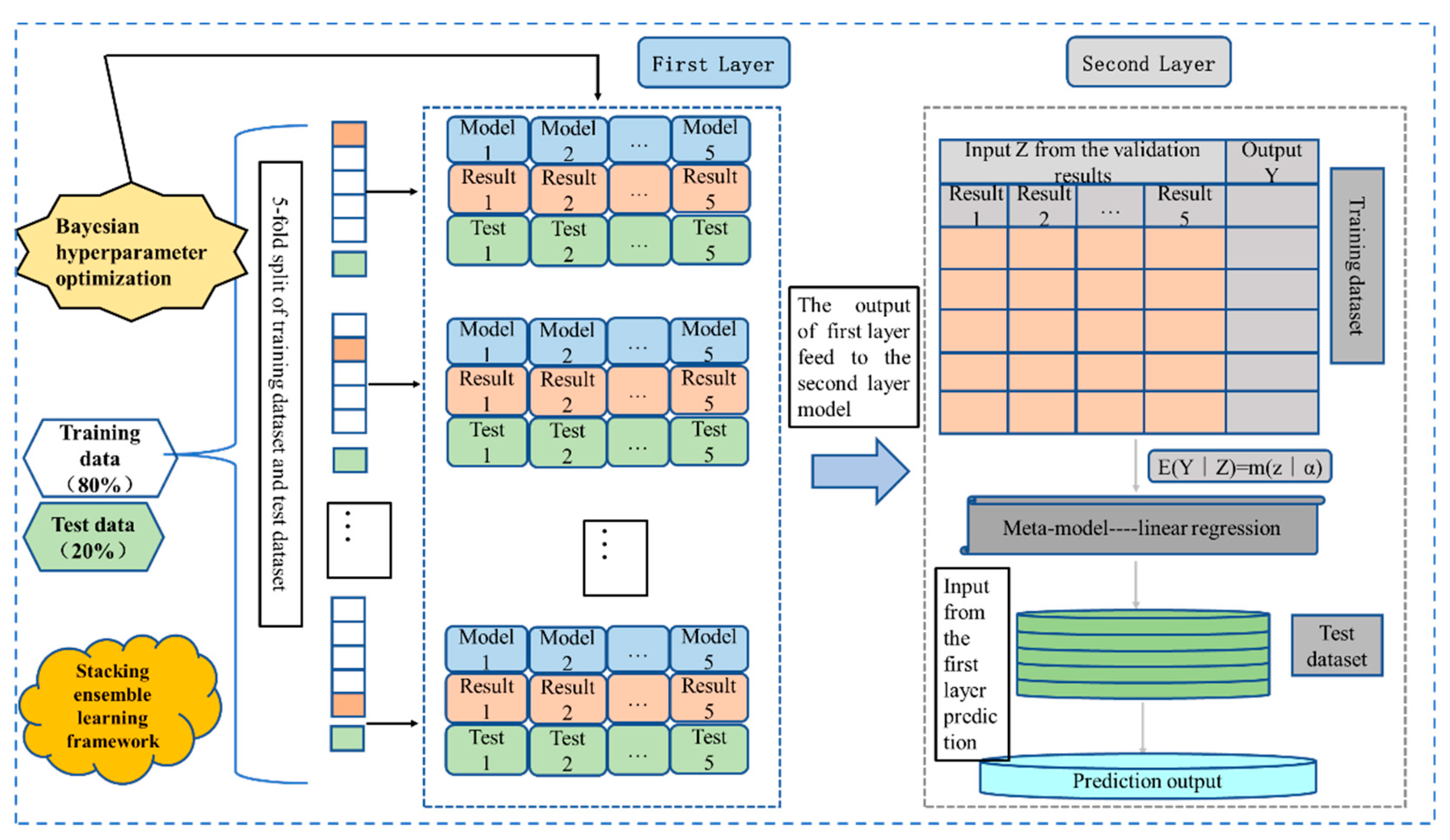
Algorithms with different principles and structures can measure data from different perspectives, complementing each other. The diversity and excellent forecasting ability of the base-model is crucial to enhance the generalization and regression performance of the stacking ensemble learning framework. Generally, the first layer of the stacking learning framework selects three to five base learners. Too few learners have little effect on the performance of the integrated model; too many learners will cause redundancy of the model structure and an increase in computing cost, which is not conducive to the improvement of prediction accuracy. In this paper, 12 candidate models are trained and tested on the same dataset, and 5 models with better prediction performance in terms of the R² evaluation index are selected as base learners. The base-models adaptively selected may vary for different datasets as the module of base-model selection in Figure 1.

K-fold cross-validation is applied to prevent meta-model overfitting of the training data and enhance the generalization performance of the model. Cross-validation is a resampling method used to evaluate machine learning models, and K-fold means that a given data is spilt into K separate folds. One-fold is used to train the model, and K-1 folds are used to validate, and then an individual estimation is obtained by averaging the results of K evaluations [28]. The model can be trained and validated on each fold data, increasing the model’s fitness. That is to say, the input data to the meta-model is the out-of-fold predictions from multiple base-models. The overall framework of the proposed ensemble model for renewable energy output power forecasting is displayed in Figure 1; the procedure can be summarized as follows:

(1)

Twelve candidate models are trained and tested to select five base-models by evaluating the R² index.

For each base-model:

• Select a 5-fold split of the training dataset;
• Evaluate using 5-fold cross-validation;
• Tune hyperparameters using the Bayesian optimal method;
• Store all out-of-fold predictions.

(2)

Fit a meta-model on the out-of-fold predictions by linear regression.

(3)

Evaluate the model on a holdout prediction dataset.

3. Methodology

Ensemble learning is a machine learning method that combines a series of base learners according to certain rules to obtain a strong learner, presenting a more robust performance than a single model. Ensemble techniques, including bagging, boosting and stacking, are popular and widely used in renewable energy generation prediction and load forecasting [29,30,31].

3.1. Regression Method Based on Boosting Learning

The boosting learning methods fit multiple weak learners on different versions of the training dataset, and then combines the predictions of the weak learners sequentially with different weights until a suitable strong learner is achieved [32]. Tree-based boosting methods mainly include ADA, GBRT, XGB and LGBM.

AdaBoost uses the Cart tree as the base learner and conducts multiple iterations of learning to minimize the loss by changing the weights of base learners in each iterative step [27,32]. GBRT uses a gradient boosting algorithm based on ADA and follows a shrinkage and regularization approach, which effectively improves the accuracy and stability of the prediction [27,33].

The XGB method adds several optimizations and refinements to the original GBRT, making the creation ensembles more straightforward and more generative. The details of XGB can be found in [20,22,27]. LGBM is a modified XGB algorithm proposed by Microsoft in 2017. Gradient-based one-sided sampling (GOSS) and exclusive feature bundling (EFB) are used to enhance its histogram algorithm and decision tree growth strategy, improving the computing speed, stability, and robustness without reducing accuracy [18].

Taking LGBM as an example, a given dataset $D=\left\{(x_i,y_i):i=1\cdots N\right\}$, the input timeseries $x_i$, and the output $y_i$, constructing the nonlinear mapping $y=f(x)$. Denoting the loss function $L(y,f(x))={(y-f(x))}^2$, the objective of model training is to find the function $f*(x)=\underset{f}{{\displaystyle \arg \min }}{E}_{y,x}L(y,f(x))$. The LGBM algorithm (Algorithm 1) steps can be written as follows:

Algorithm 1 LGBM Regression

(1) Input: Training data $D=\left\{(x_i,y_i):i=1\cdots N\right\}$, iteration number M, loss function $L(y,f(x))={(y-f(x))}^2$; (2) Output: $f_M(x)={\displaystyle \sum _{m=1}^M{\delta }_{m}T(x;{\Theta }_m)}$; (3) Initialize $f_0(x)=\underset{\delta }{\arg \min }{\displaystyle \sum _{i=1}^{N}L(y_i,\delta )}$; For $m=1$ to M (a) For $i=1,2,\cdots ,N$, calculating $g_m(x_i)=-{\left[\frac{\partial L(y_i,f(x_i))}{\partial f(x_i)}\right]}_{f(x)=f_{m-1(x)}}$ (b) Fit a regression tree $T(x;{\Theta }_m)$ to $g_{\mathrm{m}}(x_i)$; (c) Find the better $({\delta }_m, {\Theta }_m)$ through $\underset{\delta ,\Theta }{\arg \min }{\displaystyle \sum _{i=1}^{N}L(y_i,f_{m-1}(x_i)+\delta T(x_i;\Theta ))}$ , and calculate ${\Theta }_{\mathrm{m}}=\arg \underset{\Theta ,\delta }{\min }{\displaystyle \sum _{i=1}^N{[-g_m(x_i)-\delta T(x_i; \Theta )]}^2}$; (d) Calculate the optimal weight for each regression tree $T(x;{\Theta }_m)$, ${\delta }_m=\arg \underset{\delta }{\min }{\displaystyle \sum _{i=1}^{N}L[y_i,f_{m-1}(x_i)+\delta T(x_i, {\Theta }_m)}$; (e) Update model: $f_m(x)=f_{m-1}(x)+{\delta }_{m}T(x;{\Theta }_m)$ end for (4) Output $f_{\mathrm{m}}(x)$.

where initial $f_0(x)=\delta$, $\delta =\frac{1}{N}{\displaystyle \sum _{i=1}^N{y}_i}$, presenting the initial weight of the regression tree; and Θ is the parameters of the regression tree.

3.2. Regression Method Based on Bagging Learning

The bagging ensemble uses bootstrap replicates to obtain multiple different samples of the same training dataset as new training sets, and fits a decision tree on each new set. Due to perturbed training, the predictions for all of the created decision trees can reduce variance. Then, the predictions are combined, which can improve accuracy and prevent overfitting of the bagging method [34,35].

Random forest RF is an extension of bagging technology, which also uses bootstrap sampling to build a large number of training sample sets and fit different decision trees. Unlike bagging, to make the individual decision trees differ, RF estimates the input feature and then selects a number of samples as split candidates at each node [35]. Out-of-bag (OOB) error estimation is employed to construct the forest, which can ensure unbiasedness and reduce forecast variance [36,37].

An extra regression tree (ET) is developed as an extension of the RF approach, which employs a classical top-down procedure to construct an ensemble of unpruned regression trees. As well as RF, a subset of features is randomly selected to train each base estimator. Unlike RF, ET randomly selects the best feature with the corresponding value to split the node. Additionally, ET employs the total training dataset to train each regression tree in the forest [36]. These differences are likely to reduce overfitting, as interpreted in [38].

3.3. Other Regression Models

Linear regression is widely used in statistics to quantitatively analyze the dependence relationship between two or more variables. Basic linear regression is used to describe the linear relationship between variables. The least-square method is a commonly used algorithm to train the linear regression model. Elastic net is developed as an extension of linear regression. It adds L1 and L2 regularization parameters, which integrate the benefits of the least absolute shrinkage, selection operator (lasso) and ridge, resulting in a better performance for prediction [39].

K-nearest neighbor regression (KNN) carries out prediction by measuring the distance of a sample’s nearest neighbor. KNN finds the K-nearest neighbors of a sample and assigns the mean value of some features of these neighbors to the sample. In other words, the mean value is the prediction value of the sample. The time series for wind power and PV power has a specific correlation in the time dimension. Theoretically, the KNN method is suitable for wind and PV power forecasting, and has been applied to renewable energy forecasting [40,41,42].

Support vector regression (SVR) is used to solve regression problems by adopting kernel functions to construct non-linear mapping. That is to say, the input space is mapped into a higher dimensional feature space, and a linear regression is performed in the feature space. The traditional empirical risk minimization principle only minimizes the training error. In contrast, SVR uses the structure risk minimization principle to minimize an upper boundary of the total generalization error with a certain confidence level. SVR is highly effective in solving non-linear problems, even with small sample events, and is popular in wind and PV power forecasting [36,43].

3.4. Stacking Ensemble

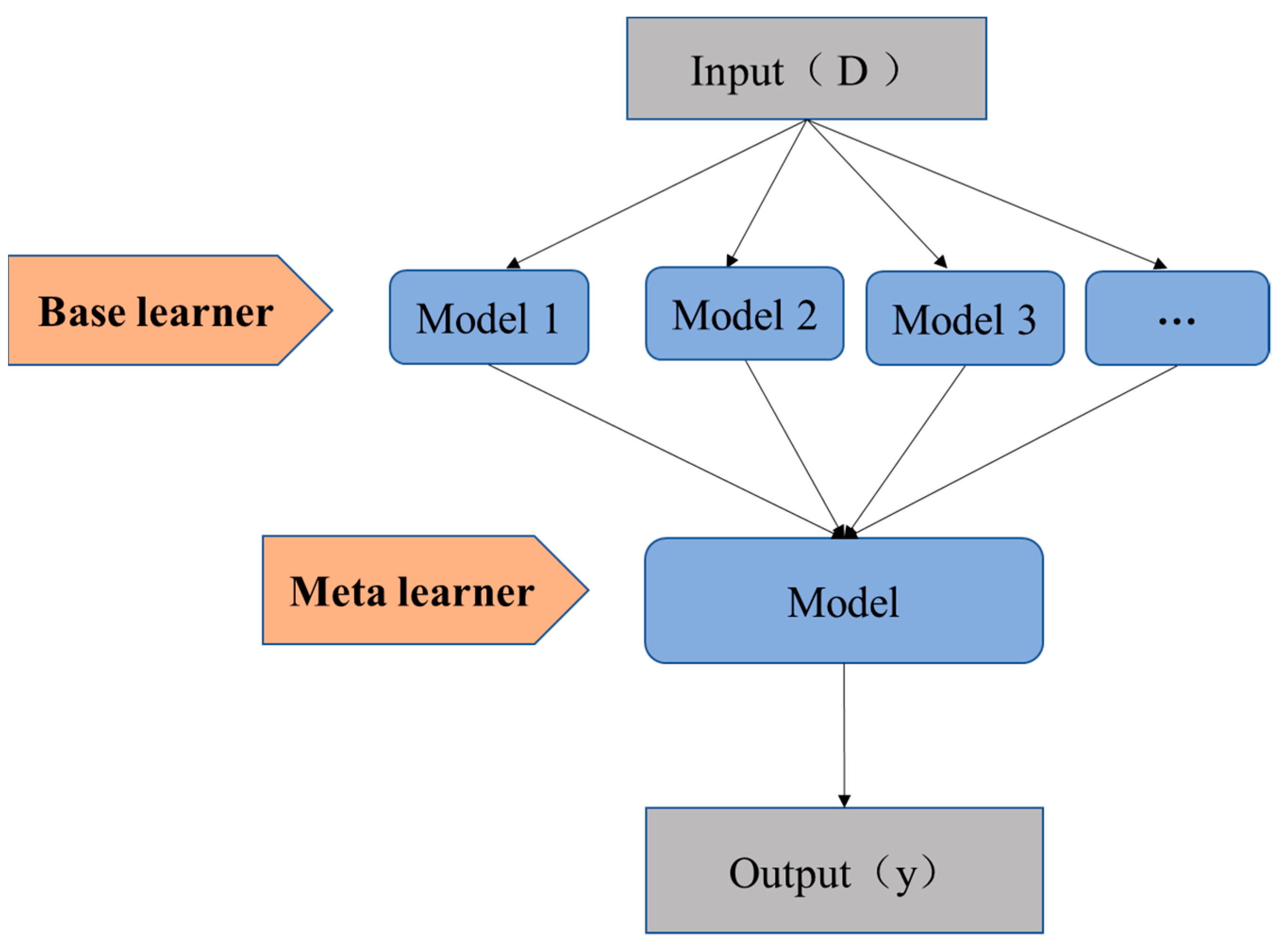
Stacking ensemble trains different base-models on the same dataset. Then, it uses a meta-model to combine the predictions generated via the base-models to achieve the ultimate predictions [44]. The two-layer stacking ensemble learning framework is displayed in Figure 2. The first layer consists of multiple different basic learner models, and the input is the original data training set. The second layer is called the meta learner; the prediction from the first layer model is fed to the meta-model to make the ultimate prediction. The meta learner integrates the prediction ability of the basic learner model to improve the performance of stacking ensemble learning.

Given the input dataset $D=(x_1,\cdots ,x_i,\cdots ,x_m)$, the dataset is divided into the training dataset, test dataset and validation dataset. $Z_h$ is the h-th base-model of the first layer. The prediction output of the $Z_h$ model on the validation set is $Z_h(x_i)$, and the prediction result of the $Z_h$ model on validation dataset is presented using $Z^{*}{}_h(x_i)$. The output $Z_h(x_i)$ of the first layer model as a new training set is fed to the meta-model $Z$, and $Z^{*}{}_h(x_i)$ as a test of the meta-model. The ultimate forecasting result can be written as follows:

$$y_i=Z(Z_1(x_i)/Z^{*}{}_1(x_i),\cdots ,Z_h(x_i)/Z^{*}{}_h(x_i),\cdots ,Z_n(x_i)/Z^{*}{}_n(x_i))$$

(1)

3.5. Bayesian Hyperparameters Optimization

Bayesian optimization is derived from the famous Bayes theorem, which uses a probabilistic surrogate model to fit the objective function and selects the most “potential” evaluation point via the maximum acquisition function. The procedure of parameter optimization can reduce unnecessary sampling and make full use of the complete historical information to improve the search efficiency, and then obtain a global approximate optimal solution with low evaluation cost [45,46]. Traditional optimization algorithms, such as grid search, particle swarm optimization, simulated annealing, etc., are not suitable for machine learning methods with large-scale parameters due to their expensive computing costs [46].

In this paper, the hyperparameters of the base-models and meta-model are tuned using Bayesian optimization, as shown in Figure 3. Firstly, a hyperparameter space $\Theta \in \Lambda$, such as leaf nodes of the tree, and learning depth are defined. Given the dataset $D=\{(x_0,y_0),\cdots ,(x_{i-1},y_{i-1})\}$, Bayesian global optimization can be described as ${\Theta }^{*}\in \arg {\max }_{\Theta \in \Lambda }F(\Theta )$, where ${\Theta }^{*}$ is the optimal hyperparameter and $F(\Theta )$ is the objective function, indicating the loss of validation of the model with the hyperparameters. Assuming that $F(\Theta )$ cannot be observed directly, we can only obtain this by noise observations $Y(\Theta )=F(\Theta )+\epsilon ,\epsilon \sim N(0,{\sigma }^2{}_{noise})$. The construction of a surrogate function and the selection of an acquisition function are critical technologies for Bayesian optimization. A surrogate function is built to express assumptions about the function to be optimized, and an acquisition function is selected to determine the next evaluation point. In this paper, the tree Parzen estimator (TPE) is employed to model the densities using a kernel density estimator, instead of directly modeling the objective function F by a probabilistic model $p(f|D)$ [47,48]. More details about Bayesian optimization are discussed in [45,46,47,48].

4. Results and Discussions

4.1. Data

Wind speed (WS) and direction (WD), as the main meteorological features affecting wind output power, are selected as the inputs for the wind power prediction model, and wind power (WP) as the output. Data was collected from the SCADA system of a wind farm, located in central China. The installed capacity of the wind farm is 200 MW, and the rated power of each wind turbine is 2 MW. The historical data covers the whole year of 2020 with a 15-min time resolution, divided into four datasets depending on different seasons with 8832 samples in each season. Figure 4 gives an example of the historical dataset in Spring.

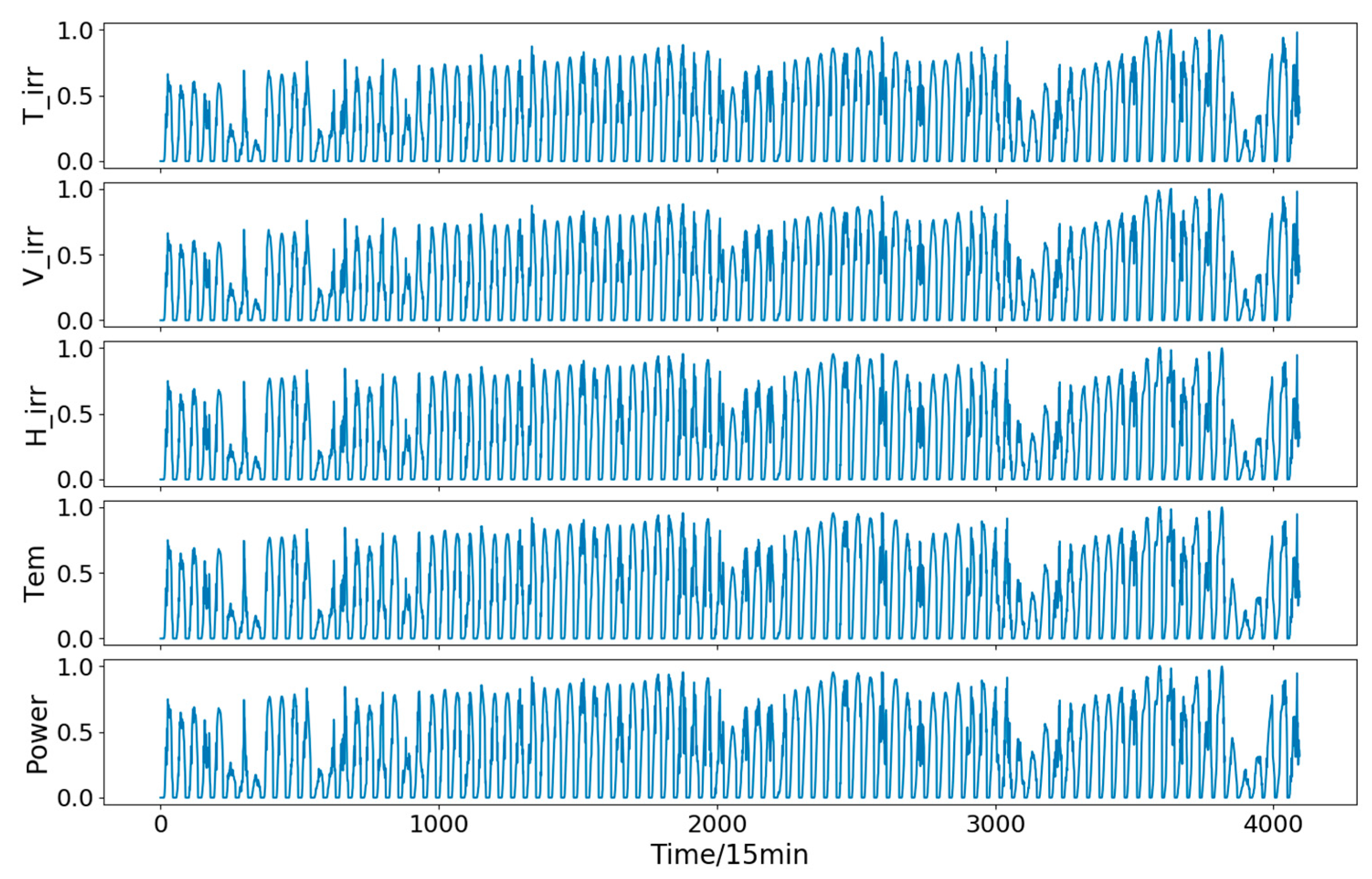
In the PV power model, the main meteorological features affecting PV output power are selected as the inputs of the prediction model, which include total irradiance (T_irr), normal vertical irradiance (V_irr), horizontal irradiance (H_irr) and temperature (Tem). The data is derived from a PV power station with 130 MW located in central China. Due to the characteristics of PV output power, the historical data from 07:00 to 18:00 is defined as effective, which consists of the whole year of 2020 with a 15-min time resolution. The dataset of each season contains 4095 time points. An example of the historical data for spring is shown in Figure 5.

From Figure 4 and Figure 5, we can see that there are some differences between the characteristics of wind power and solar power. The time series of wind power is random, whereas the solar power time series has specific rules to follow. During the day, PV power can be generated only when the PV cells are radiated by the sun. At night, the output power from the PV station is 0. The diversity between the two datasets can be used to verify the model’s universality.

4.2. Data Standardization and Evaluation Indices

To reduce interference from outliers and differences from different data dimensions and ensure fairness of the forecast, the principle of maximum and minimum is applied for normalization to (0, 1). It can be written as follows:

$${\tilde{x}}_{ij}=\frac{x_{ij}-x_{i\min }}{x_{i\max }-x_{i\min }}(i=1,2,\cdots ,I;j=1,2,\cdots ,J)$$

(2)

where: $x_{ij}$ is the $j$-th sample of the variable $i$-th, and ${\tilde{x}}_{ij}$ is the corresponding normalization value; $x_{i.\max }$ and $x_{i.\min }$ represent the maximum and minimum values of $i$-th variable, respectively.

Root-mean-square error (RMSE), mean absolute error (MAE) and determination coefficient R² are usually selected as the evaluation indices of the prediction model [49,50]. The smaller the RMSE and MAE values, the smaller the prediction error will be. The determination coefficient R² measures the similarity between the actual and predicted values. The larger the value, the better the model fitting effect. These indices can be described as follows:

$$\mathrm{RMSE}=\sqrt{\frac{1}{N}{\displaystyle \sum _{i=1}^N{(P_i-\stackrel{Ù}{P_i})}^2}}$$

(3)

$$\mathrm{MAE}=\frac{1}{N}{\displaystyle \sum _{i=1}^N\left|P_i-\stackrel{Ù}{P_i}\right|}$$

(4)

$${\mathrm{R}}^2=1-\frac{{\displaystyle \sum {(P_i-\stackrel{\wedge }{P_i})}^2}}{{\displaystyle \sum {(P_i-{\stackrel{-}{P}}_i)}^2}}$$

(5)

where, P_i and $\stackrel{\wedge }{P_i}$ present the measured and prediction values, respectively; ${\overline{P}}_i$ is the average of measured value and N is the number of samples.

4.3. Model Selection and Hyperparameter Optimization

As shown in Figure 1 of Section 2, 12 candidate models are simulated on four data cases to select 5 better base-models. The original data is divided into a training dataset (80% data) and a validation dataset (20% data). For the different datasets in spring, summer, autumn, and winter, five models with higher scores are adaptively selected as the base-models according to the R² evaluation index. Especially, if the R² scores of the models are the same, the RMSE and MAE indices are used for further evaluation. The training and testing of the proposed model using Python 3.6 are conducted on a computer with Intel(R) Core (TM)i7-8565, [email protected] GHz, RAM 8.00 GB.

The results of the wind power prediction on the validation dataset are displayed in

Table 1. Evaluation indices of the base-models for wind power prediction.

Method	Indices	Spring Dataset	Summer Dataset	Autumn Dataset	Winter Dataset
LR	RMSE	0.189	0.135	0.205	0.237
	MAE	0.166	0.114	0.123	0.208
	R2	0.579	0.52	0.49	0.315
ELAN	RMSE	0.294	0.209	0.295	0.287
	MAE	0.269	0.188	0.273	0.259
	R2	−0.016	−0.151	−0.063	0
SVR	RMSE	0.169	0.109	0.111	0.174
	MAE	0.129	0.079	0.08	0.134
	R2	0.662	0.689	0.851	0.634
DT	RMSE	0.21	0.159	0.136	0.236
	MAE	0.139	0.116	0.085	0.167
	R2	0.48	0.335	0.775	0.322
KNN	RMSE	0.163	0.128	0.11	0.188
	MAE	0.112	0.095	0.068	0.136
	R2	0.686	0.569	0.853	0.573
ADA	RMSE	0.159	0.123	0.136	0.174
	MAE	0.132	0.103	0.104	0.142
	R2	0.701	0.604	0.776	0.633
Bagging	RMSE	0.166	0.126	0.113	0.197
	MAE	0.115	0.094	0.071	0.142
	R2	0.677	0.581	0.845	0.526
RF	RMSE	0.16	0.125	0.109	0.19
	MAE	0.111	0.092	0.068	0.138
	R2	0.698	0.591	0.854	0.562
ET	RMSE	0.173	0.133	0.117	0.202
	MAE	0.117	0.098	0.073	0.146
	R2	0.649	0.538	0.834	0.505
GBRT	RMSE	0.147	0.113	0.105	0.165
	MAE	0.106	0.08	0.065	0.124
	R2	0.746	0.667	0.867	0.667
XGB	RMSE	0.151	0.116	0.104	0.175
	MAE	0.105	0.084	0.062	0.128
	R2	0.731	0.648	0.869	0.628
LGBM	RMSE	0.145	0.112	0.104	0.167
	MAE	0.102	0.08	0.063	0.125
	R2	0.754	0.673	0.868	0.662

. Five base-models are selected with higher R² scores and lower RMSE and MAE values. For the spring dataset, the selected base-models are LGBM, GBRT, XGB, ADA, and RF, with corresponding R² values of 0.754, 0.746, 0.731, 0.701, and 0.698, respectively. For the summer dataset, the base-models are SVR, LGBM, GBRT, XGB, and ADA, with corresponding R² values of 0.689, 0.673, 0.667, 0.648 and 0.604 respectively. The base modes and their R² scores for the autumn dataset are XGB-0.869, GBRT-0.868, LGBM (0.867), RF (0.854), and KNN (0.853). For the winter dataset, they are GBRT (0.667), LGBM (0.662), ADA (0.633), SVR (0.634), and XGB (0.628). The R² scores of the same model vary greatly on a different dataset, such as LGBM, GBRT, and XGB, which indicate that a single forecasting model has certain limitations for different data. In addition, for the winter and summer datasets, the R² scores of all models are lower; the RMSE and MAE values are higher than those for the spring and autumn datasets, which is closely related to the fluctuation characteristics of the original data of wind speed, direction, and power.

The results for PV power forecast are listed in

Table 2. Evaluation index of independent models for solar power prediction.

Method	Indices	Spring Dataset	Summer Dataset	Autumn Dataset	Winter Dataset
LR	RMSE	0.157	0.12	0.167	0.162
	MAE	0.117	0.095	0.121	0.128
	R2	0.711	0.858	0.381	0.759
ELAN	RMSE	0.302	0.334	0.226	0.331
	MAE	0.255	0.303	0.187	0.299
	R2	−0.07	−0.096	−0.137	−0.004
SVR	RMSE	0.147	0.111	0.148	0.118
	MAE	0.095	0.076	0.107	0.097
	R2	0.746	0.879	0.515	0.872
DT	RMSE	0.154	0.153	0.154	0.128
	MAE	0.112	0.103	0.105	0.073
	R2	0.723	0.771	0.474	0.849
KNN	RMSE	0.187	0.116	0.132	0.101
	MAE	0.111	0.08	0.092	0.062
	R2	0.589	0.868	0.611	0.906
ADA	RMSE	0.148	0.118	0.142	0.121
	MAE	0.095	0.096	0.099	0.094
	R2	0.743	0.862	0.555	0.865
Bagging	RMSE	0.134	0.107	0.137	0.111
	MAE	0.084	0.082	0.094	0.067
	R2	0.791	0.887	0.581	0.888
RF	RMSE	0.144	0.105	0.132	0.107
	MAE	0.092	0.073	0.091	0.064
	R2	0.758	0.892	0.615	0.896
ET	RMSE	0.178	0.116	0.138	0.113
	MAE	0.106	0.078	0.096	0.068
	R2	0.627	0.868	0.576	0.883
GBRT	RMSE	0.163	0.108	0.132	0.1
	MAE	0.106	0.076	0.089	0.062
	R2	0.688	0.886	0.613	0.908
XGB	RMSE	0.168	0.107	0.134	0.102
	MAE	0.111	0.078	0.091	0.065
	R2	0.669	0.888	0.604	0.904
LGBM	RMSE	0.142	0.106	0.137	0.107
	MAE	0.092	0.074	0.094	0.064
	R2	0.762	0.889	0.58	0.894

. For the spring dataset, the five models with higher R² scores are bagging (0.791), LGBM (0.762), RF (0.758), SVR (0.746), and ADA (0.743). Similarly, the base-models with higher R² scores are bagging (0.791), LGBM (0.762), RF (0.758), SVR (0.746), and ADA (0.743). For the autumn dataset, the highest R² scores are RF (0.615), GBRT (0.613), KNN (0.611), XGB (0.604), and bagging (0.581). For the winter dataset, the highest R² scores are GBRT (0.908), KNN (0.906), XGB (0.904), RF (0.896), and LGBM (0.894). The R² values of the ELAN model for wind power prediction and PV power prediction on all datasets are negative, which indicate that the model is unsuitable for renewable prediction. Like wind power forecasting, the evaluation indices of a model for PV power forecasting on different datasets are different. For all 12 models, the R² scores on the winter dataset are the highest, and RMSE and MAE values are the lowest, followed by summer, spring, and autumn.

Due to the significant difference between wind power and PV power time series, the base-models selected are also different, indicating the universality of different algorithms on different data. For example, the RF model is selected as the base-model on all four datasets for PV power prediction, whereas it is selected only on spring and autumn data for wind power forecasting, indicating that the performance of the RF method has certain limitations for data with stronger fluctuations. Similarly, the bagging method is selected only in wind power forecasting. We can see the variations among these base-models for different cases in Table 1 and Table 2.

With the base-model selected; the next step is to select the meta-model. Taking wind power prediction as an example, the RF, XGB, GBRT, LGBM, and LR models with higher R² scores on four datasets in the above base-model experiments are tested and verified as meta-models, respectively. The results are shown in

Table 3. Evaluation index of different meta-models.

Model	Indices	Spring Dataset	Summer Dataset	Autumn Dataset	Spring Dataset
LR	RMSE	0.137	0.104	0.098	0.158
	MAE	0.095	0.072	0.06	0.115
	R2	0.759	0.681	0.878	0.678
RF	RMSE	0.156	0.117	0.108	0.181
	MAE	0.111	0.086	0.066	0.136
	R2	0.715	0.639	0.857	0.604
GBRT	RMSE	0.161	0.122	0.113	0.184
	MAE	0.112	0.089	0.071	0.136
	R2	0.697	0.61	0.843	0.587
XGB	RMSE	0.149	0.113	0.104	0.174
	MAE	0.104	0.081	0.063	0.128
	R2	0.74	0.662	0.868	0.632
LGBM	RMSE	0.152	0.117	0.106	0.175
	MAE	0.107	0.085	0.065	0.129
	R2	0.729	0.638	0.863	0.627

. It can be seen that the RMSE and MAE values of the linear model as the meta-model are lower and R² scores are higher on each dataset than the other models. Therefore, the linear model is selected as the meta-model in this paper. In a similar manner, the LR model as the meta-model for PV power prediction on four seasons has better prediction accuracy than the other models.

In order to improve the prediction performance of the basic learner model, the Bayesian global optimization method is adopted to optimize the main parameters of these base-models, and the range of parameters are preset as listed in

Table 4. Hyperparameters of the different base learner models.

Model	Hyperparameters	Range	Model	Hyperparameters	Range
KNN	n_neighbors	1–20	SVR	svr_c	0.1–100
	weights	uniform		svr_gamma	0.01–1.0
RF	n_estimators	10–200	GBRT	n_estimators	10–200
	max_depth	10–200		subsample	0.1–1.0
	min_samples_split	1–10		min_samples_split	1–20
	min_samples_leaf	1–10		min_samples_leaf	1–20
LGBM	n_estimators	10–200	XGB	n_estimators	10–200
	max_depth	1–10		max_depth	10–200
	num_leaves	1–20		min_child_weight	1–10
	learning_rate	1–20		subsample	0.1–1.0
	subsamples	0.1–1.0		learning_rate	0.1–1.0
ADA	n_estimators	10–200	Bagging	n_estimators	10–200
	learning_rate	0.1–1.0		max_samples	1–10

. For different datasets, the optimal parameters of a model may be different. In practical application, the hyperparameter optimization of the model can use offline training and online prediction to save calculation costs and improve the efficiency of the model prediction.

4.4. Wind Power Forecasting and Results Analysis

The single base-model is employed as a benchmark for comparing with the proposed stacking ensemble model. The evaluation index values on four test datasets are shown in Figure 4. The last day of each season, namely 29 February, 31 May, 31 August, and 31 December, is selected as the forecast day. The wind power forecast curve is shown in Figure 6.

In Figure 6, the base-models adaptively selected for each dataset are different in the four seasons. Furthermore, the RMSE and MAE values of the stacking ensemble method are lower than all the selected single base-models. In winter, the RMSE and MAE values of the stacking ensemble method are 0.152 and 0.102, respectively, which are the largest compared with the other three seasons. Nevertheless, its prediction error is still much smaller than the benchmarks, such as the SVR, XGB, GBRT, ADA, and LGBM methods, of which the RMSE and MAE values are 0.169 and 0.13; 0.181 and 0.132; 0.164 and 0.122; 0.168 and 0.134; 0.17 and 0.124, respectively, indicating its excellent stability and robustness. The GBRT model is selected as the base-model in all four datasets, and its error values and R² scores are less than the stacking ensemble model, indicating that the prediction performance of GBRT has a certain stability and robustness. In addition, the R² score values of the stacking ensemble model are higher than those of the single base-models for all datasets. Taking the winter case as an example, the R² score of the stacking ensemble method is 0.702, which is the lowest for the four seasons. Nevertheless, it is still much higher than the benchmark models, demonstrating its outstanding performance, i.e., the improvement in its prediction accuracy and an enhancement of its generalization ability. From Figure 6, the prediction error for autumn is the smallest, followed by summer, spring, and winter, consistent with the characteristics of data with weaker fluctuations. It can be concluded that when the input data at some time point fluctuates greatly, the accurate prediction ability of the stacking ensemble model needs to be improved. However, compared to all the benchmark models for different datasets, the prediction performance of the proposed method is still superior.

The prediction curves of the stacking ensemble model and the comparison benchmarks with 96 time points for the selected prediction day covering four seasons are shown in Figure 7. The stacking ensemble model can better track the actual output power change trend than the single benchmark, indicating better prediction performance. In Figure 7a,c,d for winter, their prediction curves are flat in some time periods due to the weak fluctuation of the input data, including wind speed and direction. Thus, the true values closely follow the actual values. In Figure 7c for autumn, the true measured power values of the predicted day have higher fluctuations. According to the input data, wind speed and direction are random in the range of 48–96 time points, and the wind speed reaches a limit of 14~15 m/s at some time points. Therefore, the predicted power values during this time period deviate from the real measured power. However, compared to the benchmark models, the prediction curve of the stacking ensemble model is closer to the true measured values. It demonstrates that the stacking ensemble model integrates multiple algorithms with different principles, adaptively tracking changes in the datasets. Compared with the benchmark models, the proposed model for wind power forecasting has a better fitting performance and can produce more accurate point predictions along with better generalization performance and stability.

4.5. PV Power Forecasting and Results Analysis

Similar to the wind power forecasting cases, the proposed stacking ensemble model is further validated by forecasting the output power of a PV station. The division of the dataset and selection of the forecast day are the same as the case of wind power prediction. The evaluation index values and prediction curves are presented in Figure 8 and Figure 9.

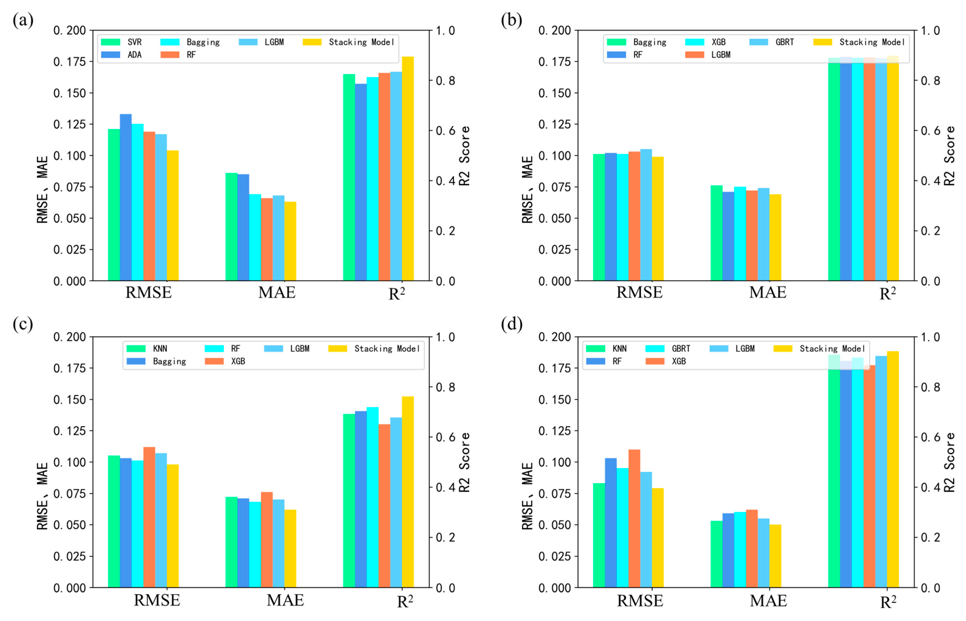
In Figure 8, the base-model adaptively selected for photovoltaic power prediction is different from that for wind power prediction. For example, in spring, the base-models for photovoltaic prediction are SVR, bagging, LGBM, ADA, and RF, while for wind power prediction, the base-models are ADA, XGB, GBRT, RF, and LGBM, demonstrating the different performance of the different models in data mining. Furthermore, the proposed stacking ensemble model has a lower prediction error and higher R² scores than the other comparison models for all the study cases. Taking the autumn dataset as an example, in Figure 8c, the RMSE and MAE values of the stacking ensemble model are 0.098 and 0.062, respectively, which are higher than the other three seasons; its R² score is 0.762 and is the lowest in all the four seasons. Nevertheless, compared to the benchmark models, its forecasting error is the lowest and its R² score is the highest, indicating the prediction superiority of the proposed method.

Due to the diversity of the data characteristics, the prediction error and fitting score in the different seasons vary. In spring, summer, autumn, and winter, the RMSE values are 0.104, 0.099, 0.098, and 0.079, respectively; the MAE values are 0.063, 0.069, 0.062, and 0.05, respectively; and R² scores are 0.894, 0.895, 0.762, and 0.942, respectively, which fully illustrate the ability of the data-driven stacking ensemble model to deep mine potential data.

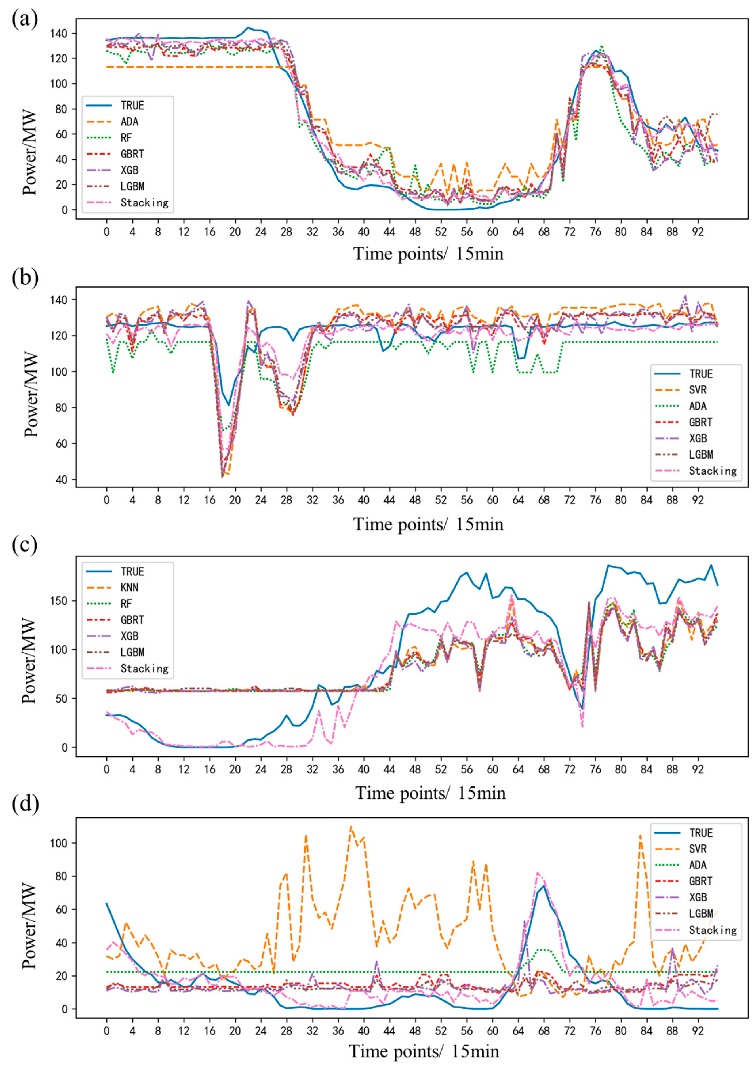
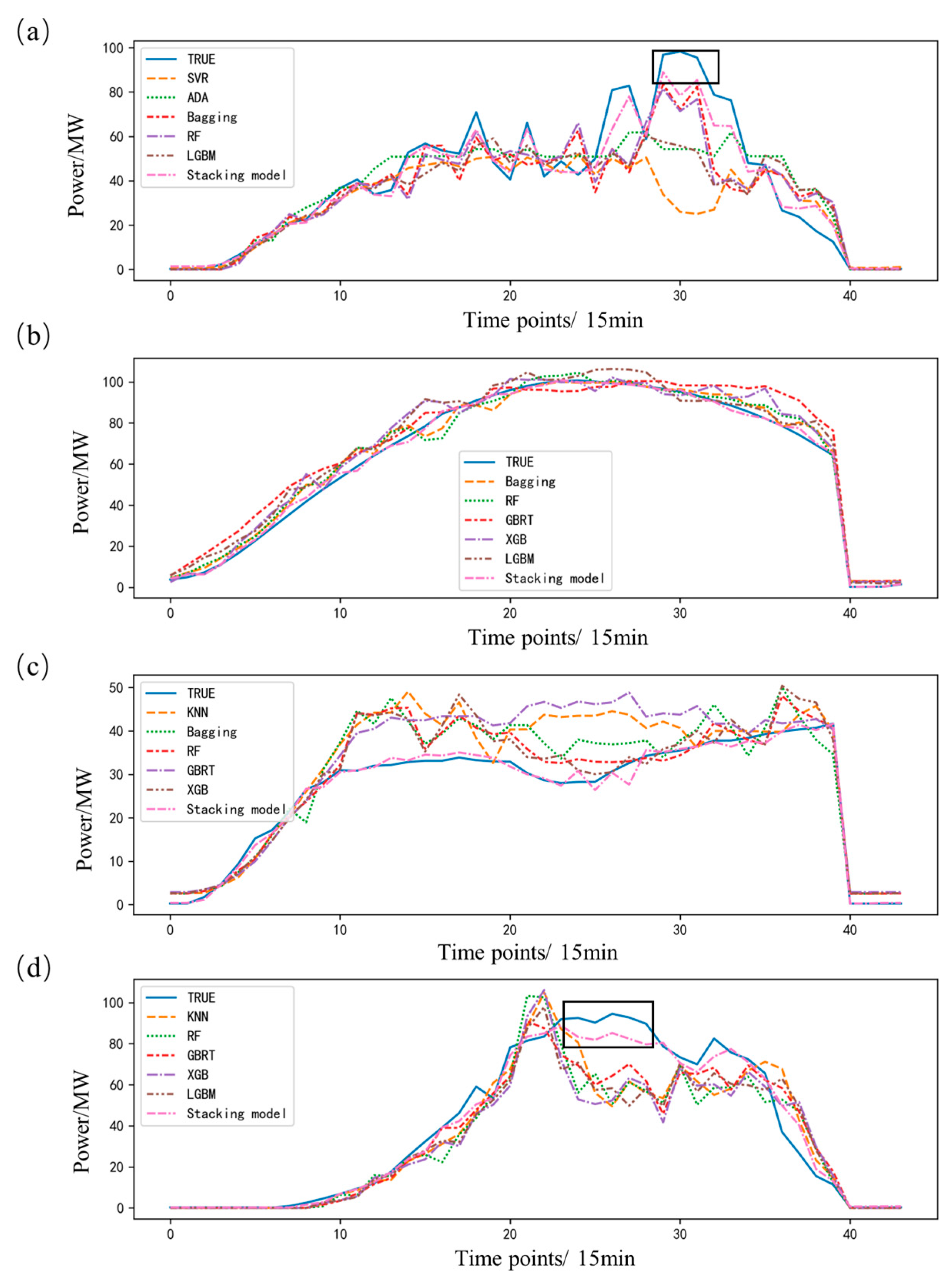
Figure 9 shows the prediction curves of the stacking ensemble model and the comparison models on the prediction day. From sub-graph (b) summer and (c) autumn, the real measured values of PV power have little variation, and the prediction curves of the stacking ensemble model closely follow the true output power curves, indicating a high prediction accuracy. In sub-graph (a) spring and (d) winter, the actual power value of the predicted day has greater fluctuations due to the variation of the input datasets. Therefore, there is a certain gap between the predicted values and the actual measured values, while the overall trends of the prediction curve follow the changes of the actual measured power curve, indicating the effectiveness and adaptiveness of the stacking ensemble method for PV power forecasting. In addition, for all datasets, at times with low PV output power, the prediction values of the proposed stacking model are similar to those of the benchmark model, indicating the difficulty of prediction at low power points. However, at times with high PV output, especially at time periods with large fluctuations (black box mark in sub-figures (a) spring and (d) winter), the prediction curves of the proposed stacking model more closely follow the true power curve, indicating the significant superiority and reliability of the proposed method for PV power prediction.

5. Conclusions

In this paper, an adaptive, data-driven stacking ensemble model is proposed for the output power prediction of renewable energy, including wind power and PV power. The proposed model is validated using datasets collected from an actual wind farm and PV station. The following conclusions can be drawn:

(1)

The models with different algorithm principles can deeply mine the space and structural characteristics of multi-dimensional heterogeneous datasets from multiple perspectives, realizing the performance complementarity among algorithms. The proposed stacking ensemble learning framework can track the dynamic changes within data, combining multiple base-models to improve the forecasting accuracy, as well as the generalization ability and adaptability.

(2)

The cross-validation and Bayesian hyperparameter optimization methods are used in the model training, which can effectively improve the model’s prediction accuracy.

(3)

The linear model is employed as a meta-model to integrate base-models. The weight of each base-model is determined by the minimum cross-validation error principle, which can further improve the model’s prediction accuracy without increasing the model’s complexity or calculation cost.

References

1. Mlilo, N.; Brown, J.; Ahfock, T. Impact of intermittent renewable energy generation penetration on the power system networks—A review. Technol. Econ. Smart Grids Sustain. Energy 2021, 6, 1–19. [Google Scholar] [CrossRef]
2. Wan, C.; Cao, Z.; Lee, W.J.; Song, Y.; Ju, P. An Adaptive Ensemble Data Driven Approach for Nonpara-metric Probabilistic Forecasting of Electricity Load. IEEE Trans. Smart Grid 2021, 12, 5396–5408. [Google Scholar] [CrossRef]
3. Sanjari, M.J.; Gooi, H.B.; Nair, N.-K.C. Power Generation Forecast of Hybrid PV–Wind System. IEEE Trans. Sustain. Energy 2019, 11, 703–712. [Google Scholar] [CrossRef] [Green Version]
4. Zhang, Y.; Le, J.; Liao, X.; Zheng, F.; Li, Y. A novel combination forecasting model for wind power integrating least square support vector machine, deep belief network, singular spectrum analysis and locality-sensitive hashing. Energy 2019, 168, 558–572. [Google Scholar] [CrossRef]
5. Yu, X.; Wang, Y.; Wu, L.; Chen, G.; Wang, L.; Qin, H. Comparison of support vector regression and extreme gradient boosting for decomposition-based data-driven 10-day streamflow forecasting. J. Hydrol. 2019, 582, 124293. [Google Scholar] [CrossRef]
6. Hanifi, S.; Liu, X.; Lin, Z.; Lotfian, S. A Critical Review of Wind Power Forecasting Methods—Past, Present and Future. Energies 2020, 13, 3764. [Google Scholar] [CrossRef]
7. Hao, Y.; Tian, C. A novel two-stage forecasting model based on error factor and ensemble method for multi-step wind power forecasting. Appl. Energy 2019, 238, 368–383. [Google Scholar] [CrossRef]
8. Rafati, A.; Joorabian, M.; Mashhour, E.; Shaker, H.R. High dimensional very short-term solar power forecasting based on a data-driven heuristic method. Energy 2021, 15, 119647. [Google Scholar] [CrossRef]
9. Yu, C.; Li, Y.; Bao, Y.; Tang, H.; Zhai, G. A novel framework for wind speed prediction based on recurrent neural networks and support vector machine. Energy Convers. Manag. 2018, 178, 137–145. [Google Scholar] [CrossRef]
10. Hong, Y.-Y.; Rioflorido, C.L.P.P. A hybrid deep learning-based neural network for 24-h ahead wind power forecasting. Appl. Energy 2019, 250, 530–539. [Google Scholar] [CrossRef]
11. Qing, X.; Niu, Y. Hourly day-ahead solar irradiance prediction using weather forecasts by LSTM. Energy 2018, 148, 461–468. [Google Scholar] [CrossRef]
12. Zhang, J.; Yan, J.; Infield, D.; Liu, Y.; Lien, F.-S. Short-term forecasting and uncertainty analysis of wind turbine power based on long short-term memory network and Gaussian mixture model. Appl. Energy 2019, 241, 229–244. [Google Scholar] [CrossRef] [Green Version]
13. Ahmad, M.W.; Mourshed, M.; Rezgui, Y. Tree-based ensemble methods for predicting PV power generation and their comparison with support vector regression. Energy 2018, 164, 465–474. [Google Scholar] [CrossRef]
14. Zheng, H.; Feng, Y.; Li, X.; Yang, H.; Lv, W.; Li, S. Investigation on Molecular Dynamics Simulation for Predicting Kinematic Viscosity of Natural Ester Insulating Oil. IEEE Trans. Dielectr. Electr. Insul. 2022, 29, 1882–1888. [Google Scholar] [CrossRef]
15. Munawar, U.; Wang, Z. A Framework of Using Machine Learning Approaches for Short-Term Solar Power Forecasting. J. Electr. Eng. Technol. 2020, 15, 561–569. [Google Scholar] [CrossRef]
16. Zhang, H.; Zhu, T. Stacking Model for Photovoltaic-Power-Generation Prediction 2022. Sustainability 2022, 14, 5669. [Google Scholar] [CrossRef]
17. Torres-Barrán, A.; Alonso, Á.; Dorronsoro, J.R. Regression tree ensembles for wind energy and solar radiation prediction. Neurocomputing 2019, 326-327, 151–160. [Google Scholar] [CrossRef]
18. Kumari, P.; Toshniwal, D. Extreme gradient boosting and deep neural network based ensemble learning approach to forecast hourly solar irradiance. J. Clean. Prod. 2021, 279, 123285. [Google Scholar] [CrossRef]
19. Sansine, V.; Ortega, P.; Hissel, D.; Hopuare, M. Solar Irradiance Probabilistic Forecasting Using Machine Learning, Metaheuristic Models and Numerical Weather Predictions. Sustainability 2022, 14, 15260. [Google Scholar] [CrossRef]
20. Kumari, P.; Toshniwal, D. Long short term memory–convolutional neural network based deep hybrid approach for solar irradiance forecasting. Appl. Energy 2021, 295, 117061. [Google Scholar] [CrossRef]
21. Abdellatif, A.; Mubarak, H.; Ahmad, S.; Ahmed, T.; Shafiullah, G.M.; Hammoudeh, A.; Abdellatef, H.; Rahman, M.M.; Gheni, H.M. Forecasting Photovoltaic Power Generation with a Stacking Ensemble Model. Sustainability 2022, 14, 11083. [Google Scholar] [CrossRef]
22. Jiajun, H.; Chuanjin, Y.; Yongle, L.; Huoyue, X. Ultra-short term wind prediction with wavelet transform, deep belief network and ensemble learning. Energy Convers. Manag. 2020, 205, 112418. [Google Scholar] [CrossRef]
23. Wang, H.-Z.; Li, G.-Q.; Wang, G.-B.; Peng, J.-C.; Jiang, H.; Liu, Y.-T. Deep learning based ensemble approach for probabilistic wind power forecasting. Appl. Energy 2017, 188, 56–70. [Google Scholar] [CrossRef]
24. Persson, C.; Bacher, P.; Shiga, T.; Madsen, H. Multi-site solar power forecasting using gradient boosted regression trees. Sol. Energy 2017, 150, 423–436. [Google Scholar] [CrossRef]
25. Fan, J.; Wang, X.; Wu, L.; Zhou, H.; Zhang, F.; Yu, X.; Lu, X.; Xiang, Y. Comparison of Support Vector Machine and Extreme Gradient Boosting for predicting daily global solar radiation using temperature and precipitation in humid subtropical climates: A case study in China. Energy Convers. Manag. 2018, 164, 102–111. [Google Scholar] [CrossRef]
26. Shao, H.; Deng, X.; Cui, F. Short-term wind speed forecasting using the wavelet decomposition and AdaBoost technique in wind farm of East China. IET Gener. Transm. Distrib. 2016, 10, 2585–2592. [Google Scholar] [CrossRef]
27. Ribeiro, M.H.D.M.; da Silva, R.G.; Moreno, S.R.; Mariani, V.C.; dos Santos Coelho, L. Efficient bootstrap stacking ensemble learning model applied to wind power generation forecasting. Int. J. Electr. Power Energy Syst. 2022, 136, 107712. [Google Scholar] [CrossRef]
28. Sáez, J.A.; Romero-Béjar, J.L. Impact of Regressand Stratification in Dataset Shift Caused by Cross-Validation. Mathematics 2022, 10, 2538. [Google Scholar] [CrossRef]
29. Da Silva, R.G.; Ribeiro, M.H.D.M.; Moreno, S.R.; Mariani, V.C.; dos Santos Coelho, L. A novel decomposition-ensemble learning framework for multi-step ahead wind energy forecasting. Energy 2021, 216, 119174. [Google Scholar] [CrossRef]
30. Liu, H.; Tian, H.-Q.; Li, Y.-F.; Zhang, L. Comparison of four Adaboost algorithm based artificial neural networks in wind speed predictions. Energy Convers. Manag. 2015, 92, 67–81. [Google Scholar] [CrossRef]
31. Zheng, H.; Cui, Y.; Yang, W.; Li, J.; Ji, L.; Ping, Y.; Hu, S.; Chen, X. An Infrared Image Detection Method of Substation Equipment Combining Iresgroup Structure and CenterNet. IEEE Trans. Power Deliv. 2022, 37, 4757–4765. [Google Scholar] [CrossRef]
32. Huang, H.; Jia, R.; Shi, X.; Liang, J.; Dang, J. Feature selection and hyper parameters optimization for short-term wind power forecast. Appl. Intell. 2021, 2, 1–19. [Google Scholar] [CrossRef]
33. Xia, R.; Gao, Y.; Zhu, Y.; Gu, D.; Wang, J. An Efficient Method Combined Data-Driven for Detecting Electricity Theft with Stacking Structure Based on Grey Relation Analysis. Energies 2022, 15, 7423. [Google Scholar] [CrossRef]
34. Agrawal, R.K.; Muchahary, F.; Tripathi, M.M. Ensemble of relevance vector machines and boosted trees for electricity price forecasting—ScienceDirect. Appl. Energy 2019, 250, 540–548. [Google Scholar] [CrossRef]
35. Fan, J.; Yue, W.; Wu, L.; Zhang, F.; Cai, H.; Wang, X.; Lu, X.; Xiang, Y. Evaluation of SVM, ELM and four tree-based ensemble models for predicting daily reference evapotranspiration using limited meteorological data in different climates of China. Agric. For. Meteorol. 2018, 263, 225–241. [Google Scholar] [CrossRef]
36. Müller, I.M. Feature selection for energy system modeling: Identification of relevant time series information. Energy AI 2021, 4, 100057. [Google Scholar] [CrossRef]
37. Breiman, L. Random forests. Mach Learn. 2001, 45, 532. [Google Scholar]
38. Geurts, P.; Ernst, D.; Wehenkel, L. Extremely randomized trees. Mach. Learn. 2006, 63, 3–42. [Google Scholar] [CrossRef] [Green Version]
39. Long, H.; Zhang, Z.; Su, Y. Analysis of daily solar power prediction with data-driven approaches. Appl. Energy 2014, 126, 29–37. [Google Scholar] [CrossRef]
40. Kusiak, A.; Zheng, H.; Song, Z. On-line monitoring of power curves. Renew. Energy 2009, 34, 1487–1493. [Google Scholar] [CrossRef]
41. Kusiak, A.; Zheng, H.; Song, Z. Models for monitoring wind farm power. Renew. Energy 2009, 34, 583–590. [Google Scholar] [CrossRef]
42. Li, L.L.; Zhao, X.; Tseng, M.L.; Tan, R.R. Short-term wind power forecasting based on support vector machine with improved dragonfly algorithm. J. Clean. Prod. 2020, 242, 118447. [Google Scholar] [CrossRef]
43. Divina, F.; Gilson, A.; Goméz-Vela, F.; García Torres, M.; Torres, J.F. Stacking Ensemble Learning for Short-Term Electricity Con-sumption Forecasting. Energies 2018, 11, 949. [Google Scholar] [CrossRef] [Green Version]
44. Wu, J.; Chen, X.Y.; Zhang, H.; Xiong, L.D.; Lei, H.; Deng, S.H. Hyperparameter optimization for machine learning models based on Bayesian optimization. J. Electron. Sci. Technol. 2019, 17, 26–40. [Google Scholar]
45. Victoria, A.H.; Maragatham, G. Automatic tuning of hyperparameters using Bayesian optimization. Evol. Syst. 2021, 12, 217–223. [Google Scholar] [CrossRef]
46. Hutter, F.; Kotthoff, L.; Vanschoren, J. Automated Machine Learning: Methods, Systems, Challenges; Springer Nature: New York, NY, USA, 2019; pp. 8–13. [Google Scholar]
47. Huang, H.; Jia, R.; Liang, J.; Dang, J.; Wang, Z. Wind Power Deterministic Prediction and Uncertainty Quantification Based on Interval Estimation. J. Sol. Energy Eng. 2021, 1, 143. [Google Scholar] [CrossRef]
48. Falkner, S.; Klein, A.; Hutter, F. BOHB: Robust and Efficient Hyperparameter Optimization at Scale. arXiv 2018, arXiv:1807.01774[P]. [Google Scholar]
49. Huang, Z.; Huang, J.; Min, J. SSA-LSTM: Short-Term Photovoltaic Power Prediction Based on Feature Matching. Energies 2022, 15, 7806. [Google Scholar] [CrossRef]
50. Ahmed, R.; Sreeram, V.; Mishra, Y.; Arif, M. A review and evaluation of the state-of-the-art in PV solar power forecasting: Techniques and optimization. Renew. Sustain. Energy Rev. 2020, 124, 109792. [Google Scholar] [CrossRef]
Figure 1. An adaptive stacking ensemble framework for renewable energy output power forecasting.
Energies 16 01963 g001aEnergies 16 01963 g001b
Figure 2. The framework of stacking ensemble learning.
Energies 16 01963 g002
Figure 3. Flow chart of the prediction model with Bayesian optimization.
Energies 16 01963 g003
Figure 4. Historical data example for spring from the wind farm.
Energies 16 01963 g004
Figure 5. Historical data example for spring from the PV station.
Energies 16 01963 g005
Figure 6. Comparison results of the different prediction models for wind power: (a) spring, (b) summer, (c) autumn, and (d) winter.
Energies 16 01963 g006
Figure 7. Wind power prediction curve of the different comparison models: (a) spring, (b) summer, (c) autumn, and (d) winter.
Energies 16 01963 g007
Figure 8. Comparison results of the different prediction models for PV power: (a) spring, (b) summer, (c) autumn, and (d) winter.
Energies 16 01963 g008
Figure 9. PV power prediction curve of the different comparison models: (a) spring, (b) summer, (c) autumn, and (d) winter.
Energies 16 01963 g009