

Maximization of Energy Efficiency by Synchronizing the Speed of Trains on a Moving Block System


Abstract
:1. Introduction
Background of the Issue
2. Related Work
- application of the minimum braking,
- application of the “experienced driver” profile,
- keeping a constant minimum speed to a target with a specified driving time,
- keeping a constant speed and driving without the application of propulsion to a target with a specific driving time,
- optimal speed profile, taking into account track profile, speed limits and time to destination.
3. Methodology
3.1. Abbreviations Used in the Publication
- PP—”preceding” train,
- PN—“following” train,
- PW—“model” train (PN moving in undisturbed traffic),
- VP—the speed of the “preceding” train,
- VN—the speed of the “following” train,
- D0—initial distance (at the beginning of the simulation) between trains,
- T—simulation duration.
3.2. Movement Situations
- maintaining a safe braking distance for PN,
- minimizing driving time for PN,
- minimizing mechanical energy consumption for PN.
3.3. Simulation
3.3.1. Contexts
- Context 1 represents a speed reduction of 20% of the maximum speed and can refer to situations of temporary signal loss in the ETCS system.
- Context 2 assumes a value of 50% of the maximum speed and may result from the occurrence of a speed restriction based on speed grading in the automatic linear interlocking system.
- Context 3 represents a speed reduction of 80% of the maximum speed and can represent the situation of transition in ETCS between SR and FS modes.
3.3.2. Variants
- Variant 1
- Variant 2
- Variant 3
- Variant 4
- Variant 5
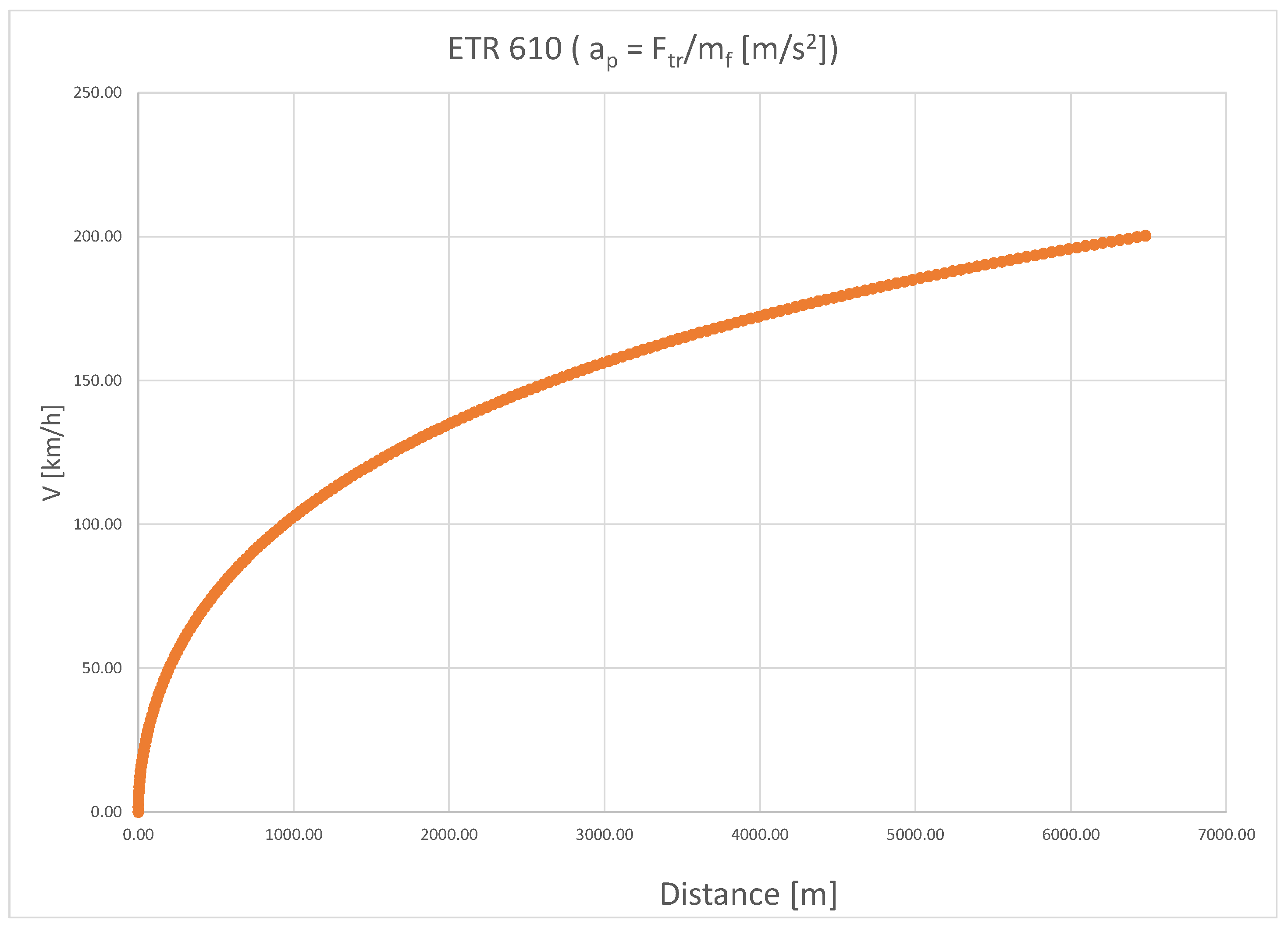
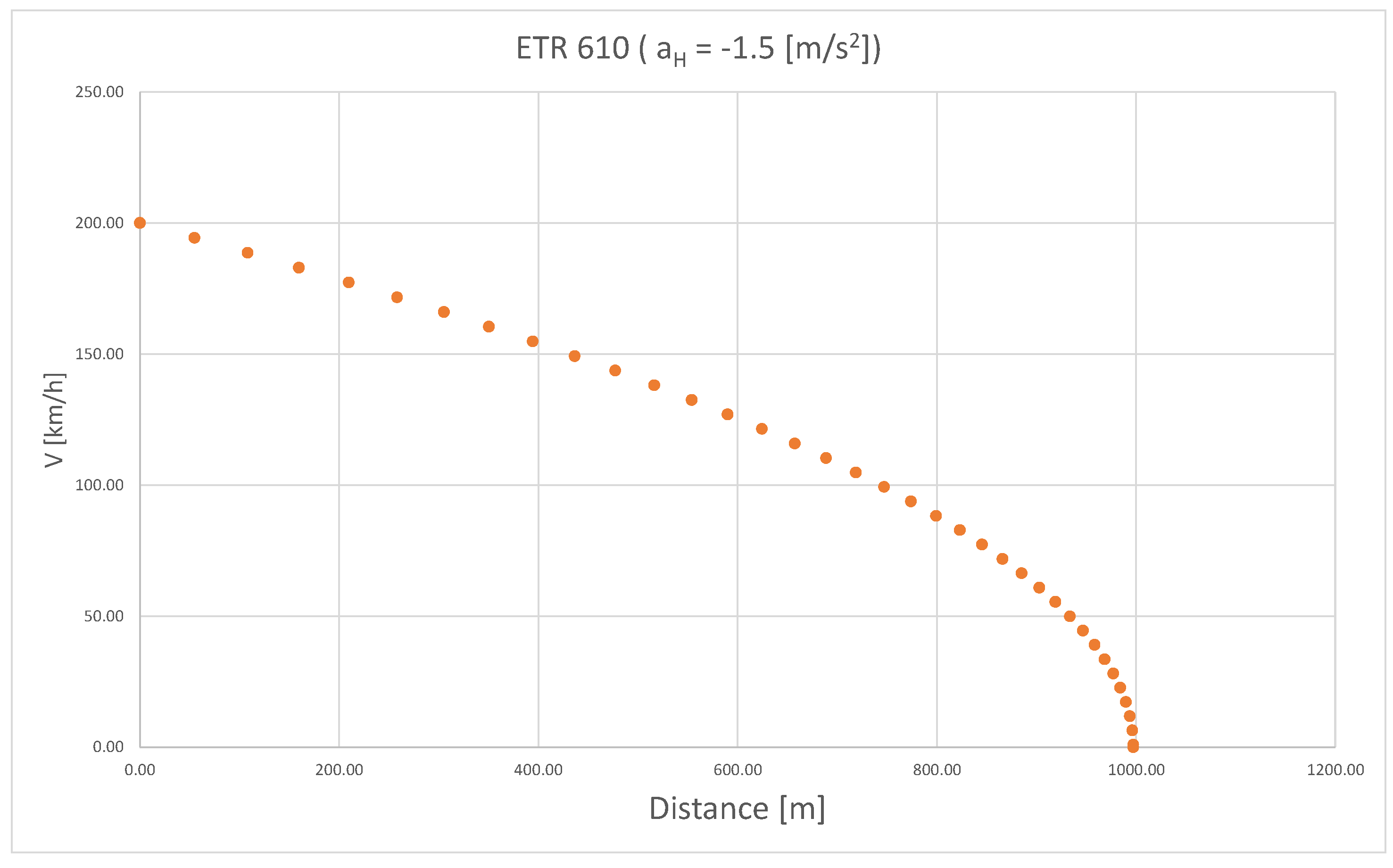
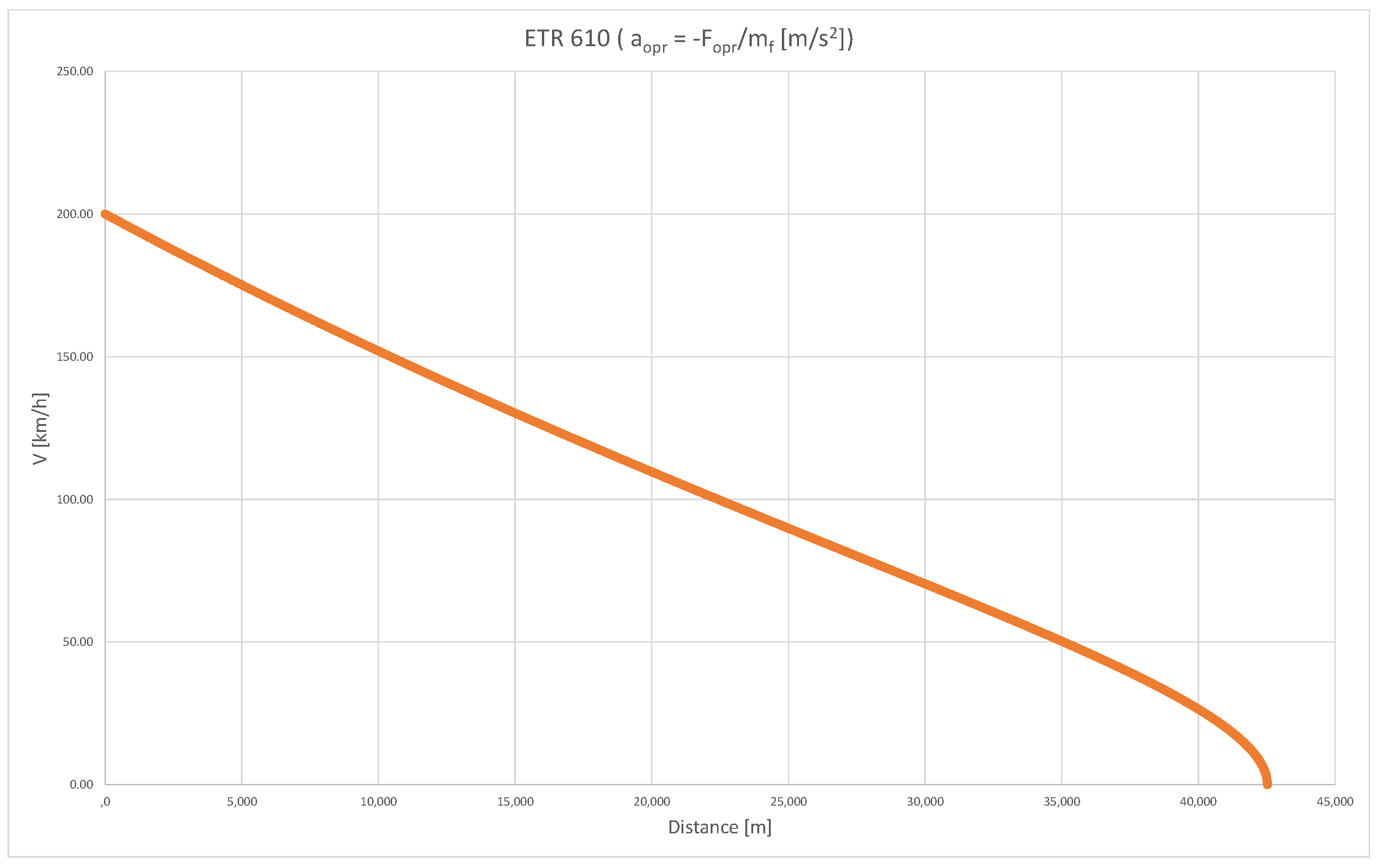
3.4. Input Data
- ar = 0.49 m/s2—average acceleration from 0 km/h to 40 km/h,
- ar = 0.49 m/s2—average acceleration from 0 km/h to 120 km/h,
- ar = 0.36 m/s2—average acceleration from 0 km/h to 160 km/h,
- ar = 0.07 m/s2—residual acceleration at 250 km/h.
3.5. Verification of Results
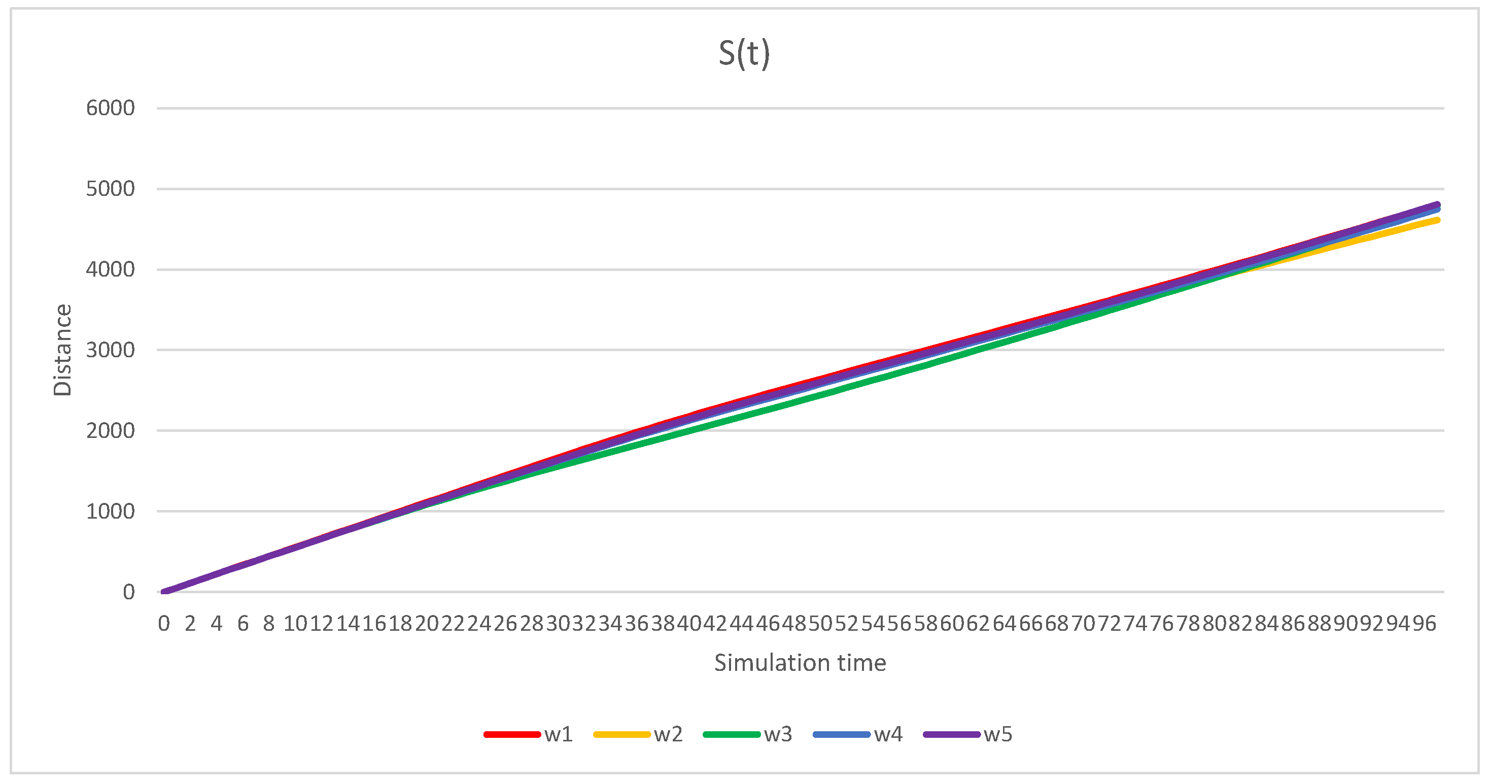
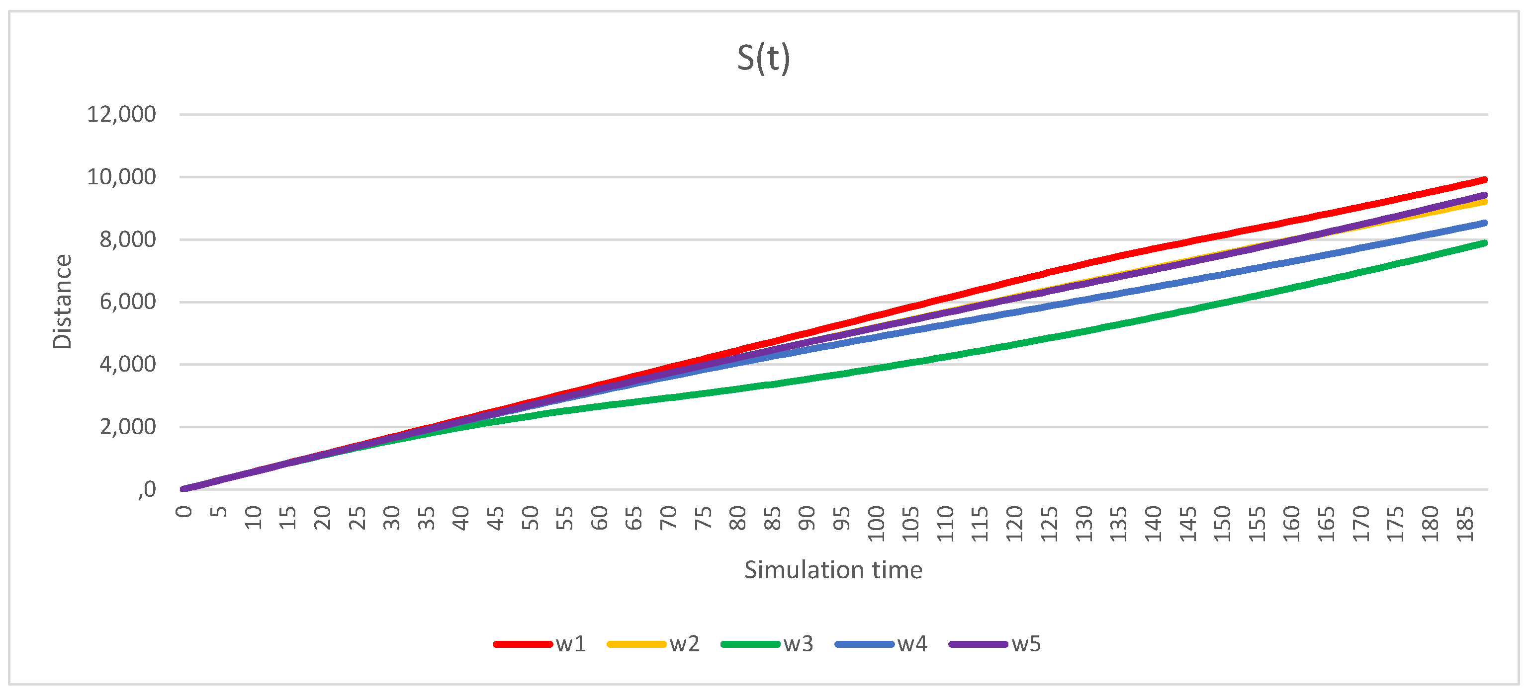
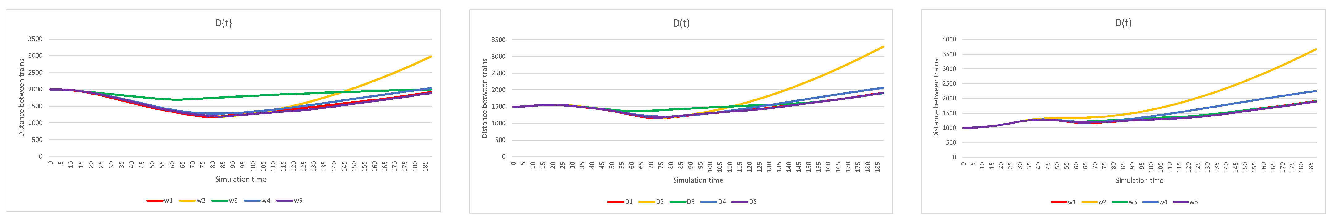
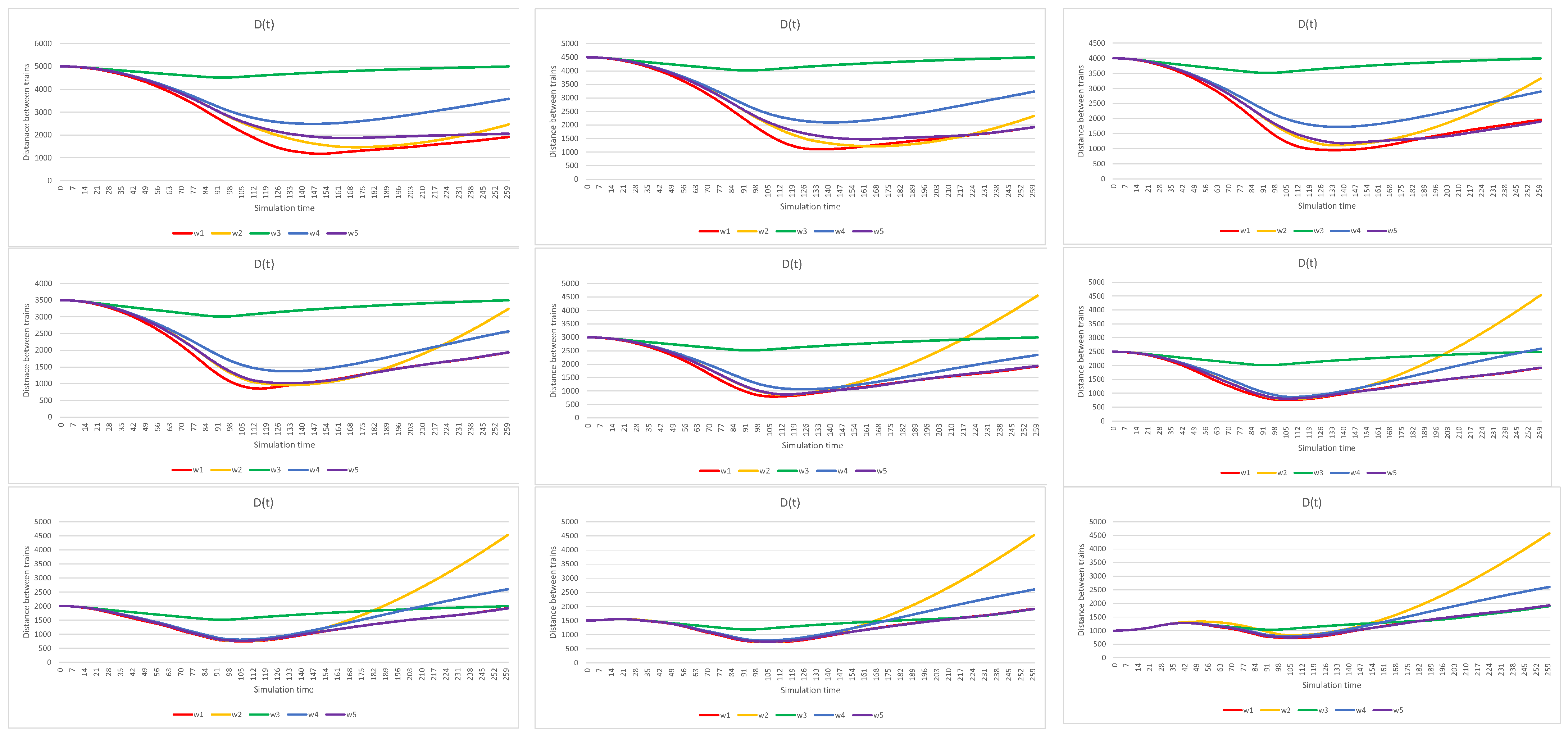
3.6. Results and Their Normalization
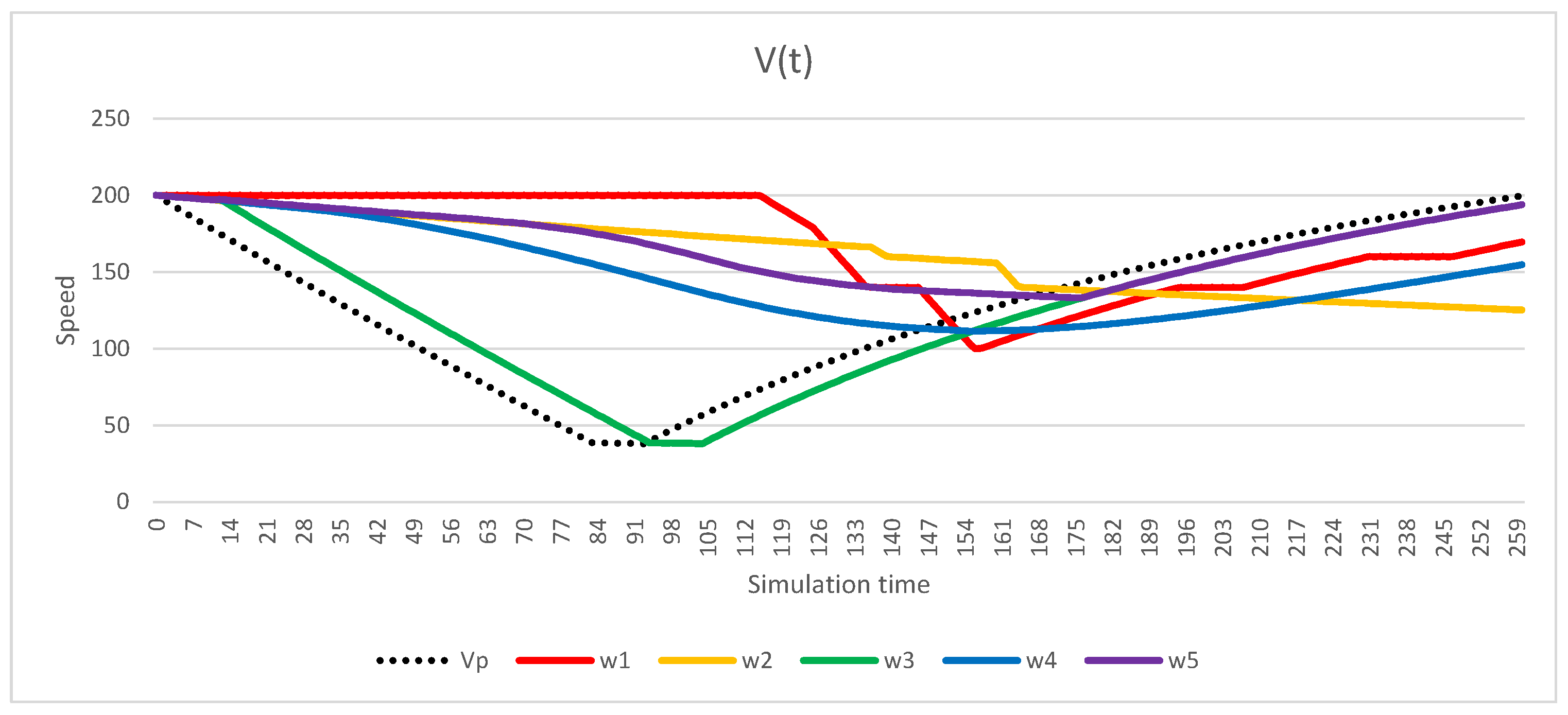
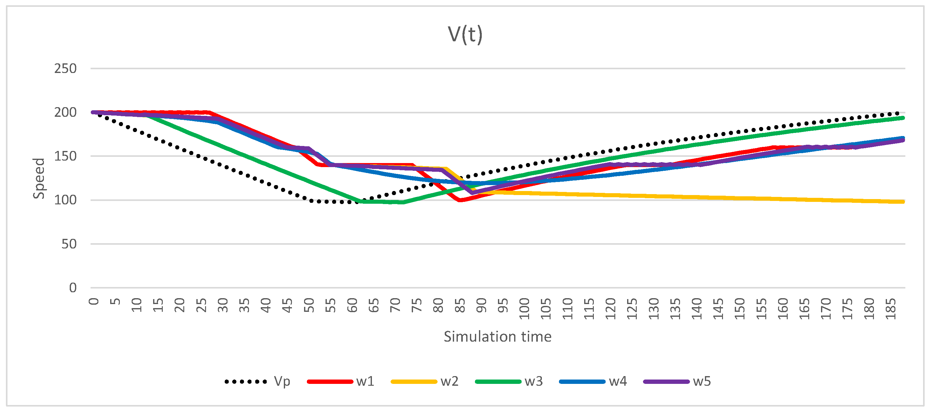
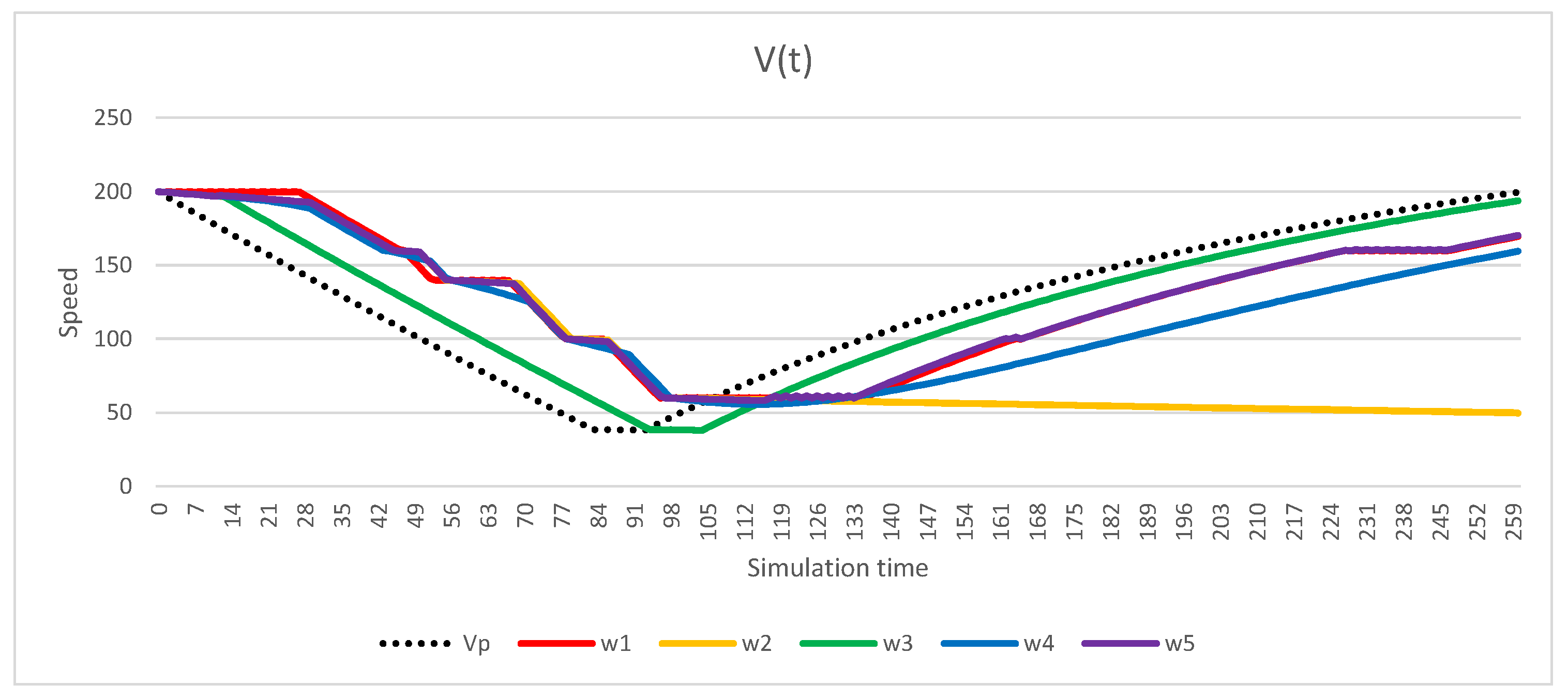
- Aligning the speed of the “following” train with the “reference” train.
- The required time TO-s1 and mechanical energy Z(∆V) necessary for PN to regain maximum speed V = Vmax (section O–s1 in Figure 6) are determined.
- Alignment of the covered distance of the “following” train with the “model” train.
- The necessary time Ts1–B and the mechanical energy Z(∆S) needed to travel the missing distance to where PW was at time t = T (section s1–B in Figure 6) are determined.
- Elimination of the resulting delay time of the “following” train to the “model” train.
- The mechanical energy Z(∆T) required for the so-called “catch-up” PW (section B–C in Figure 6) is determined, which is possible by hypothetically raising the speed above a fixed maximum speed: > Vmax.
Algorithm for Converting Time Loss into Mechanical Energy
4. Simulation Results
4.1. Description
4.2. Result
- Context 1, Dgr = 2000 m: w1 − w5 = 12.950, w2 − w5 = 26.827, w3 − w5 = 4.289, w4 − w5 = 0.028 (kWh);
- Context 2, Dgr = 4000 m: w1 − w5 = 39.120, w2 − w5 = 22.625, w3 − w5 = 205.473, w4 − w5 = 106.467 (kWh);
- Context 3, Dgr = 5000 m: w1 − w5 = 105.540, w2 − w5 = 43.178, w3 − w5 = 270.045, w4 − w5 = 129.366 (kWh).


4.3. Results in Terms of Creating a Virtual Coupling
- (1)
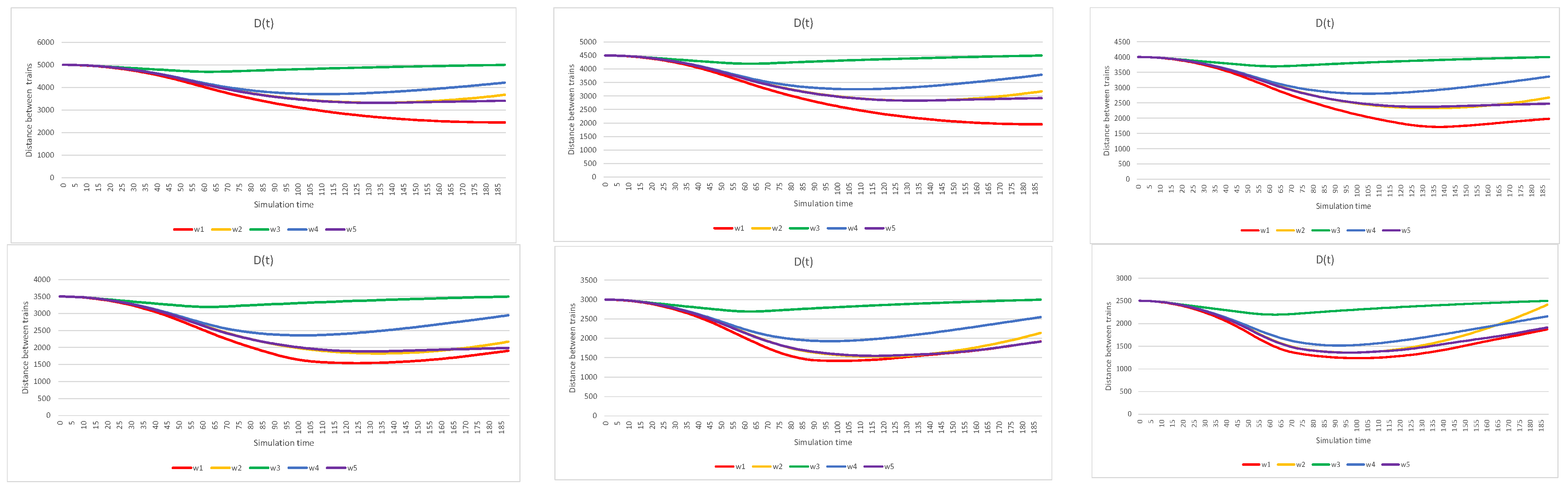
- A constant distance D(t) is maintained between PN and PP, which means the speed is equalized between the trains;
- (2)
- The solution is chosen for the shortest distance D0;
- (3)
- The V(t) curve for the PN waveform has a smooth character (small changes in speed), which indicates the smoothness of the PN movement.

- For context 1, the difference in energy consumption is: w3 − w2 = 4289 kWh,
- For context 2: w3 − w4 = 25,676 kWh,
- For context 3: w3 − w5 = 0.878 kWh,
4.4. Sensitivity Analysis
- The magnitude of the speed reduction of the PP train with respect to the PN parameters is non-linear. The difference in speed and distance loss between contexts 1 and 2 is smaller than between contexts 2 and 3.
- The factor most susceptible to context variation is the path loss (speeds stabilize at 85%), which has a key impact on the final value of time loss and ultimately on energy consumption.
- Reducing the initial distance affects energy consumption more than the context change itself. This can be seen by comparing the percentage of energy consumption for context 3 at D0 = 4 km compared to contexts 1 and 2, at D0 = 2 km. A factor contributing to this condition is the lack of smoothness of the train (dynamic speed changes).
5. Conclusions and Discussion
- Context 1: ∆Zm (w1 − w5) = 12.950 kWh;
- Context 2: ∆Zm (w1 − w5) = 39.120 kWh;
- Context 3: ∆Zm (w1 − w5) = 105.540 kWh.
Author Contributions
Funding
Data Availability Statement
Conflicts of Interest
References
- European Railway Agency. Unisig SUBSET-026 System Requirements Specification; Issue 3.6.0; European Railway Agency: Valenciennes, France, 2016.
- Wontorski, P.; Kochan, A. Komputerowe Systemy Kierowania i Sterowania Ruchem Kolejowym. Część 1: Funkcje, Elementy i Układy (Computer Systems for Directing and Controlling Railway Traffic. Part 1: Functions, Elements and Layouts); OWPW: Warszawa, Poland, 2020. [Google Scholar]
- Koper, E.; Kochan, A.; Gruba, Ł. Simulation of the Effect of Selected National Values on the Braking Curves of an ETCS Vehicle. In Development of Transport by Telematics; Mikulski, J., Ed.; Springer: Cham, Switzerland, 2019; pp. 17–31. [Google Scholar] [CrossRef]
- Mitchell, I.; Goddard, E.; Montes, F.; Stanley, P.; Muttram, R.; Coenraad, W.; Poré, J.; Andrews, S.; Lochman, L. Ertms Level 4, Train Convoys or Virtual Coupling; IRSE International Technical Committee; IRSE: London, UK, 2016. [Google Scholar]
- Quaglietta, E. Analysis of Platooning Train Operations under V2V communication-based signalling: Fundamental modelling and capacity impacts of Virtual Coupling. In Proceedings of the 98th Transportation Research Board Annual Meeting, Washington, DC, USA, 13–17 January 2019. [Google Scholar]
- Flammini, F.; Marrone, S.; Nardone, R.; Petrillo, A.; Santini, S.; Vittorini, V. Towards Railway Virtual Coupling. In Proceedings of the 2018 IEEE International Conference on Electrical Systems for Aircraft, Railway, Ship Propulsion and Road Vehicles & International Transportation Electrification Conference (ESARS-ITEC), Nottingham, UK, 7–9 November 2018. [Google Scholar]
- Niing, Z.; Ou, D.; Zhang, L. Virtual Coupling Formation Scheduling Method for Y-type Rail Transit Lines. In Proceedings of the 2022 IEEE 25th International Conference on Intelligent Transportation Systems (ITSC), Macau, China, 8–12 October 2022; pp. 3673–3678. [Google Scholar] [CrossRef]
- Wang, Q.; Chai, M.; Wang, H.; Zhang, H.; Chai, J.; Lin, B. Cloud-Based Simulated Automated Testing Platform for Virtual Coupling System. In Proceedings of the 2022 IEEE 25th International Conference on Intelligent Transportation Systems (ITSC), Macau, China, 8–12 October 2022; pp. 2738–2743. [Google Scholar] [CrossRef]
- Bin, Z.; Shijun, Y.; Lanfang, Z.; Daming, L.; Yalan, C. Energy-Efficient Speed Profile Optimization for High-Speed Railway Considering Neutral Sections. IEEE Access 2021, 9, 25090–25100. [Google Scholar] [CrossRef]
- ShangGuan, W.; Yan, X.-H.; Cai, B.-G.; Wang, J. Multiobjective optimization for train speed trajectory in CTCS high-speed railway with hybrid evolutionary algorithm. IEEE Trans. Intell. Transp. Syst. 2015, 16, 2215–2225. [Google Scholar] [CrossRef]
- Koper, E.; Kochan, A. Testing the Smooth Driving of a Train Using a Neural Network. Sustainability 2020, 12, 4622. [Google Scholar] [CrossRef]
- Wang, X.; Tang, T.; Su, S.; Yin, J.; Gao, Z.; Lv, N. An integrated energy-efficient train operation approach based on the space-time-speed network methodology. Transp. Res. Part E Logist. Transp. Rev. 2021, 150, 102323. [Google Scholar] [CrossRef]
- Wang, Y.; Zhu, S.; D’Ariano, A.; Yin, J.; Miao, J.; Meng, L. Energy-efficient timetabling and rolling stock circulation planning based on automatic train operation levels for metro lines. Transp. Res. Part C Emerg. Technol. 2021, 129, 103209. [Google Scholar] [CrossRef]
- Zhu, Q.; Su, S.; Tang, T.; Liu, W.; Zhang, Z.; Tian, Q. An eco-driving algorithm for trains through distributing energy: A Q-Learning approach. ISA Trans. 2022, 122, 24–37. [Google Scholar] [CrossRef] [PubMed]
- Houshmand, A.; Cassandras, C.G.; Zhou, N.; Hashemi, N.; Li, B.; Peng, H. Combined Eco-Routing and Power-Train Control of Plug-In Hybrid Electric Vehicles in Transportation Networks. IEEE Trans. Intell. Transp. Syst. 2022, 23, 11287–11300. [Google Scholar] [CrossRef]
- Ying, P.; Zeng, X.; Shen, T.; Wang, Y.; Ma, Z.; Wu, Y. Partial Train Speed Trajectory Optimization. In Proceedings of the 2022 IEEE 25th International Conference on Intelligent Transportation Systems (ITSC), Macau, China, 8–12 October 2022; pp. 548–553. [Google Scholar] [CrossRef]
- Fernández-Rodríguez, A.; Fernández-Cardador, A.; Cucala, A.P. Real time eco-driving of high speed trains by simulation-based dynamic multi-objective optimization. Simul. Model. Pract. Theory 2018, 84, 50–68. [Google Scholar] [CrossRef]
- Xu, B.; Lu, S.; Xue, F.; Jiang, L.; Chen, M. Adaptive Eco-Driving Strategy and Feasibility Analysis for Electric Trains with Onboard Energy Storage Devices. IEEE Trans. Transp. Electrif. 2021, 7, 1834–1848. [Google Scholar] [CrossRef]
- Fernández-Rodríguez, A.; Fernández-Cardador, A.; Cucala, A.P. Balancing energy consumption and risk of delay in high speed trains: A three-objective real-time eco-driving algorithm with fuzzy parameters. Transp. Res. Part C Emerg. Technol. 2018, 95, 652–678. [Google Scholar] [CrossRef]
- Fernández-Rodríguez, A.; Fernández-Cardador, A.; Cucala, A.P. Algorithm for Interoperable Automatic Train Operation. Appl. Sci. 2020, 10, 7705. [Google Scholar] [CrossRef]
- Mensing, F.; Trigui, R.; Bideaux, E. Vehicle trajectory optimization for application in ECO-driving. In Proceedings of the 2011 IEEE Vehicle Power and Propulsion Conference, Chicago, IL, USA, 6–9 September 2011; pp. 1–6. [Google Scholar] [CrossRef]
- Dib, W.; Chasse, A.; Moulin, P.; Sciarretta, A.; Corde, G. Optimal energy management for an electric vehicle in eco-driving applications. Control Eng. Pract. 2014, 29, 299–307. [Google Scholar] [CrossRef]
- Deng, K.; Fang, T.; Feng, H.; Peng, H.; Löwenstein, L.; Hameyer, K. Hierarchical eco-driving and energy management control for hydrogen powered hybrid trains. Energy Convers. Manag. 2022, 264, 115735. [Google Scholar] [CrossRef]
- Kochan, A. Digital Twin Concept of the ETCS application. WUT J. Transp. Eng. 2021, 131, 87–98. [Google Scholar] [CrossRef]
- Koper-Olecka, E.; Kochan, A. APM transport system concept for CPK terminals. WUT J. Transp. Eng. 2020, 130, 29–42. [Google Scholar] [CrossRef]
- Kochan, A.; Gruba, Ł. Analysis of the Migration Process in the ERTMS System from GSM Technology to LTE on the Polish Railway. In Management Perspective for Transport Telematics; Mikulski, J., Ed.; Springer: Cham, Switzerland, 2018; pp. 249–262. [Google Scholar] [CrossRef]
- Kochan, A.; Koper, E. Mathematical Model of the Movement Authority in the ERTMS/ETCS System. In Research Methods and Solutions to Current Transport Problems; Siergiejczyk, M., Krzykowska, K., Eds.; Springer: Cham, Switzerland, 2020; pp. 215–224. [Google Scholar] [CrossRef]
- Panou, K.; Tzieropoulos, P.; Emery, D. Railway Driver Advisory Systems: Evaluation of Methods, Tools and Systems. In Proceedings of the 3th WCTR, Rio de Janeiro, Brazil, 15–18 July 2013. [Google Scholar]
- Szkopiński, J.; Kochan, A. Energy Efficiency and Smooth Running of a Train on the Route While Approaching Another Train. Energies 2021, 14, 7593. [Google Scholar] [CrossRef]
- EN 14531-1:2015; Railway Applications—Methods for Calculation of Stopping and Slowing Distances and Immobilization Braking—Part 1: General Algorithms Utilizing Mean Value Calculation for Train Sets or Single Vehicles. European Standard: Brussels, Belgium, 2015.
- Shift2Rail. X2Rail-1. Start-Up Activites for Advanced Signalling and Automatition Systems. Deliverable D5.1 Moving Block System Specification. 19 July 2019. Available online: https://projects.shift2rail.org (accessed on 19 April 2022).
- SCILAB. Available online: https://www.scilab.org (accessed on 1 July 2022).
- Wawrzyniak, A. Elektryczne Pociągi Zespołowe ETR610 Serii ED250 dla PKP INTERCITY S.A.(ETR610 Electric Trainsets of the ED250 Series for PKP Intercity S.A.); Technika Transportu Szynowego: Radom, Poland, 2013. [Google Scholar]
- Durzyński, Z.; Łastowski, M. Energochłonność Pociągów Zespołowych na Duże Prędkości (Energy Consumption of High-Speed Trains); Pojazdy Szynowe: Poznań, Poland, 2010. [Google Scholar]
- Biliński, J.; Błażejewski, M.; Malczewska, M.; Szczepiórkowska, M. Opory Ruchu Pojazdów Trakcyjnych (Motion Resistance of Traction Vehicles); Technika Transportu Szynowego: Radom, Poland, 2019. [Google Scholar]


| Distance to Stopping Point (m) | Train Speed (km/h) | Deceleration Delay (m/s2) |
|---|---|---|
| 1800 | V > 160 | −0.5 |
| 1500 | V > 140 | −1.0 |
| 1200 | V > 100 | −1.0 |
| 900 | V > 60 | −1.0 |
| 100 | V > 0 | −1.5 |
| Symulation Results | Normalization Results | |||||||||
|---|---|---|---|---|---|---|---|---|---|---|
| Variant | T [s] | S [m] | V [km/h] | Zm [kWh] | Loss S [m] | Loss T [s] | Zm + Comp. S [kWh] | Comp. T [kWh] | Σ Zm [kWh] | |
| D = 5000 m | 1 | 97 | 5385 | 200 | 60.918 | 5 | 1 | 8.179 | 22.211 | 30.390 |
| 2 | 97 | 5040 | 175 | 0 | 493 | 9 | −6.108 | 74.569 | 68.461 | |
| 3 | 97 | 4785 | 194 | 88.708 | 615 | 12 | 53.752 | 88.357 | 142.109 | |
| 4 | 97 | 5012 | 181 | 17.441 | 470 | 9 | 3.377 | 74.569 | 77.946 | |
| 5 | 97 | 5114 | 194 | 36.622 | 286 | 6 | −1.616 | 59.031 | 57.415 | |
| D = 4500 m | 1 | 97 | 5385 | 200 | 60.918 | 5 | 1 | 8.179 | 22.211 | 30.390 |
| 2 | 97 | 5040 | 175 | 0 | 493 | 9 | −6.108 | 74.569 | 68.461 | |
| 3 | 97 | 4785 | 194 | 88.708 | 615 | 12 | 53.752 | 88.357 | 142.109 | |
| 4 | 97 | 5004 | 181 | 18.077 | 480 | 9 | 4.112 | 74.569 | 78.681 | |
| 5 | 97 | 5114 | 194 | 36.622 | 286 | 6 | −1.616 | 59.031 | 57.415 | |
| D = 4000 m | 1 | 97 | 5385 | 200 | 60.918 | 5 | 1 | 8.179 | 22.211 | 30.390 |
| 2 | 97 | 5040 | 175 | 0 | 493 | 9 | −6.108 | 74.569 | 68.461 | |
| 3 | 97 | 4785 | 194 | 88.708 | 615 | 12 | 53.752 | 88.357 | 142.109 | |
| 4 | 97 | 4996 | 181 | 19.261 | 487 | 9 | 5.366 | 74.569 | 79.935 | |
| 5 | 97 | 5114 | 194 | 36.622 | 286 | 6 | −1.616 | 59.031 | 57.415 | |
| D = 3500 m | 1 | 97 | 5385 | 200 | 60.918 | 5 | 1 | 8.179 | 22.211 | 30.390 |
| 2 | 97 | 5040 | 175 | 0 | 493 | 9 | −6.108 | 74.569 | 68.461 | |
| 3 | 97 | 4785 | 194 | 88.708 | 615 | 12 | 53.752 | 88.357 | 142.109 | |
| 4 | 97 | 4983 | 181 | 20.777 | 500 | 9 | 7.012 | 74.569 | 81.581 | |
| 5 | 97 | 5114 | 194 | 36.622 | 286 | 6 | −1.616 | 59.031 | 57.415 | |
| D = 3000 m | 1 | 97 | 5385 | 200 | 60.918 | 5 | 1 | 8.179 | 22.211 | 30.390 |
| 2 | 97 | 5040 | 175 | 0 | 493 | 9 | −6.108 | 74.569 | 68.461 | |
| 3 | 97 | 4785 | 194 | 88.708 | 615 | 12 | 53.752 | 88.357 | 142.109 | |
| 4 | 97 | 4964 | 180 | 22.897 | 521 | 10 | 9.335 | 79.319 | 88.654 | |
| 5 | 97 | 5114 | 194 | 36.622 | 286 | 6 | −1.616 | 59.031 | 57.415 | |
| D = 2500 m | 1 | 97 | 5385 | 200 | 60.918 | 5 | 1 | 8.179 | 22.211 | 30.390 |
| 2 | 97 | 5040 | 175 | 0 | 493 | 9 | −6.108 | 74.569 | 68.461 | |
| 3 | 97 | 4785 | 194 | 88.708 | 615 | 12 | 53.752 | 88.357 | 142.109 | |
| 4 | 97 | 4943 | 181 | 26.399 | 539 | 10 | 12.048 | 79.319 | 91.367 | |
| 5 | 97 | 5114 | 194 | 36.622 | 286 | 6 | −1.616 | 59.031 | 57.415 | |
| D = 2000 m | 1 | 97 | 4807 | 180 | 69.046 | 682 | 13 | 58.061 | 92.709 | 150.770 |
| 2 | 97 | 4616 | 151 | 0 | 1258 | 23 | 32.887 | 131.760 | 164.647 | |
| 3 | 97 | 4785 | 194 | 88.708 | 615 | 12 | 53.752 | 88.357 | 142.109 | |
| 4 | 97 | 4746 | 176 | 46.129 | 777 | 14 | 40.923 | 96.926 | 137.849 | |
| 5 | 97 | 4808 | 184 | 66.578 | 650 | 12 | 49.463 | 88.357 | 137.820 | |
| D = 1500 m | 1 | 97 | 4379 | 169 | 45.985 | 1233 | 23 | 56.866 | 131.760 | 188.626 |
| 2 | 97 | 4169 | 144 | 0 | 1817 | 33 | 45.877 | 166.355 | 212.232 | |
| 3 | 97 | 4380 | 169 | 69.829 | 1233 | 23 | 80.709 | 131.760 | 212.469 | |
| 4 | 97 | 4375 | 170 | 56.514 | 1224 | 23 | 65.386 | 131.760 | 197.146 | |
| 5 | 97 | 4383 | 169 | 67.659 | 1230 | 23 | 78.514 | 131.760 | 210.274 | |
| D = 1000 m | 1 | 97 | 3740 | 166 | 100.798 | 1907 | 35 | 121.265 | 172.968 | 294.233 |
| 2 | 97 | 2985 | 93 | 0 | 4068 | 74 | 107.212 | 291.312 | 398.524 | |
| 3 | 97 | 3757 | 167 | 102.129 | 1881 | 34 | 122.352 | 169.671 | 292.023 | |
| 4 | 97 | 3757 | 166 | 101.948 | 1883 | 34 | 122.182 | 169.671 | 291.853 | |
| 5 | 97 | 3757 | 167 | 102.129 | 1881 | 34 | 122.353 | 169.671 | 292.024 | |
| Symulation Results | Normalization Results | |||||||||
|---|---|---|---|---|---|---|---|---|---|---|
| Variant | T [s] | S [m] | V [km/h] | Zm [kWh] | Loss S [m] | Loss T [s] | Zm + Comp. S [kWh] | Comp. T [kWh] | Σ Zm [kWh] | |
| D = 5000 m | 1 | 188 | 10,436 | 200 | 116.958 | 65 | 2 | 12.851 | 32.142 | 44.993 |
| 2 | 188 | 9210 | 156 | 0 | 1634 | 30 | −20.365 | 156.287 | 135.922 | |
| 3 | 188 | 7883 | 194 | 173.578 | 2573 | 47 | 107.716 | 211.055 | 318.771 | |
| 4 | 188 | 8672 | 164 | 45.806 | 2057 | 38 | 20.199 | 182.720 | 202.919 | |
| 5 | 188 | 9474 | 194 | 72.573 | 982 | 18 | −9.158 | 113.047 | 103.889 | |
| D = 4500 m | 1 | 188 | 10,436 | 200 | 116.958 | 65 | 2 | 12.851 | 32.142 | 44.993 |
| 2 | 188 | 9210 | 156 | 0 | 1634 | 30 | −20.365 | 156.287 | 135.922 | |
| 3 | 188 | 7883 | 194 | 173.578 | 2573 | 47 | 107.716 | 211.055 | 318.771 | |
| 4 | 188 | 8600 | 164 | 50.067 | 2125 | 39 | 25.148 | 185.913 | 211.061 | |
| 5 | 188 | 9462 | 194 | 73.583 | 994 | 18 | −8.025 | 113.047 | 105.022 | |
| D = 4000 m | 1 | 188 | 9905 | 180 | 126.904 | 636 | 12 | 64.061 | 88.357 | 152.418 |
| 2 | 188 | 9210 | 156 | 0 | 1634 | 30 | −20.365 | 156.287 | 135.922 | |
| 3 | 188 | 7883 | 194 | 173.578 | 2573 | 47 | 107.716 | 211.055 | 318.771 | |
| 4 | 188 | 8523 | 165 | 55.883 | 2190 | 40 | 30.662 | 189.103 | 219.765 | |
| 5 | 188 | 9412 | 194 | 77.529 | 1044 | 19 | −3.582 | 116.880 | 113.298 | |
| D = 3500 m | 1 | 188 | 9479 | 168 | 98.21 | 1192 | 22 | 58.247 | 128.112 | 186.359 |
| 2 | 188 | 9210 | 156 | 0 | 1634 | 30 | −20.365 | 156.287 | 135.922 | |
| 3 | 188 | 7883 | 194 | 173.578 | 2573 | 47 | 107.716 | 211.055 | 318.771 | |
| 4 | 188 | 8435 | 166 | 62.788 | 2262 | 41 | 36.369 | 192.294 | 228.663 | |
| 5 | 188 | 9397 | 194 | 78.538 | 1059 | 20 | −2.426 | 120.699 | 118.273 | |
| D = 3000 m | 1 | 188 | 8963 | 170 | 117.557 | 1687 | 31 | 80.621 | 159.684 | 240.305 |
| 2 | 188 | 8742 | 142 | 0 | 2346 | 43 | 2.496 | 198.623 | 201.119 | |
| 3 | 188 | 7883 | 194 | 173.578 | 2573 | 47 | 107.716 | 211.055 | 318.771 | |
| 4 | 188 | 8334 | 168 | 71.883 | 2340 | 43 | 43.361 | 198.623 | 241.984 | |
| 5 | 188 | 8966 | 171 | 68.433 | 1669 | 31 | 29.393 | 159.684 | 189.077 | |
| D = 2500 m | 1 | 188 | 8511 | 166 | 102.981 | 2193 | 40 | 76.835 | 189.103 | 265.938 |
| 2 | 188 | 7968 | 123 | 0 | 3479 | 63 | 30.583 | 259.255 | 289.838 | |
| 3 | 188 | 7883 | 194 | 173.578 | 2573 | 47 | 107.716 | 211.055 | 318.771 | |
| 4 | 188 | 8225 | 171 | 83.677 | 2415 | 44 | 53.05 | 201.730 | 254.780 | |
| 5 | 188 | 8471 | 170 | 95.093 | 2180 | 40 | 63.073 | 189.103 | 252.176 | |
| D = 2000 m | 1 | 188 | 7968 | 169 | 139.478 | 2691 | 49 | 113.517 | 217.225 | 330.742 |
| 2 | 188 | 6907 | 99 | 0 | 5077 | 92 | 64.085 | 342.654 | 406.739 | |
| 3 | 188 | 7883 | 194 | 173.578 | 2573 | 47 | 107.716 | 211.055 | 318.771 | |
| 4 | 188 | 7848 | 171 | 97.627 | 2789 | 51 | 69.758 | 223.337 | 293.095 | |
| 5 | 188 | 7992 | 169 | 124.052 | 2676 | 49 | 98.896 | 217.225 | 316.121 | |
| D = 1500 m | 1 | 188 | 7469 | 169 | 134.317 | 3190 | 58 | 113.334 | 244.435 | 357.769 |
| 2 | 188 | 6089 | 89 | 0 | 6108 | 110 | 79.184 | 393.168 | 472.352 | |
| 3 | 188 | 7477 | 170 | 157.659 | 3174 | 58 | 135.558 | 244.435 | 379.993 | |
| 4 | 188 | 7320 | 170 | 116.645 | 3327 | 60 | 95.102 | 250.386 | 345.488 | |
| 5 | 188 | 7474 | 169 | 150.923 | 3186 | 58 | 129.899 | 244.435 | 374.334 | |
| D = 1000 m | 1 | 188 | 6974 | 169 | 158.176 | 3693 | 67 | 143.172 | 271.007 | 414.179 |
| 2 | 188 | 5214 | 84 | 0 | 7098 | 128 | 91.762 | 443.186 | 534.948 | |
| 3 | 188 | 6982 | 168 | 166.058 | 3695 | 67 | 152.029 | 271.007 | 423.036 | |
| 4 | 188 | 6632 | 167 | 133.047 | 4053 | 73 | 123.547 | 288.433 | 411.980 | |
| 5 | 188 | 6991 | 167 | 163.966 | 3695 | 67 | 150.889 | 271.007 | 421.896 | |
| Symulation Results | Normalization Results | |||||||||
|---|---|---|---|---|---|---|---|---|---|---|
| Variant | T [s] | S [m] | V [km/h] | Zm [kWh] | Loss S [m] | Loss T [s] | Zm + Comp. S [kWh] | Comp. T [kWh] | Σ Zm [kWh] | |
| D = 5000 m | 1 | 260 | 12,188 | 170 | 192.301 | 2462 | 45 | 123.194 | 204.848 | 328.042 |
| 2 | 260 | 11,641 | 126 | 0 | 3755 | 68 | −8.231 | 273.912 | 265.681 | |
| 3 | 260 | 9105 | 194 | 214.805 | 5350 | 97 | 135.775 | 356.772 | 492.547 | |
| 4 | 260 | 10,520 | 155 | 77.564 | 4338 | 79 | 46.176 | 305.692 | 351.868 | |
| 5 | 260 | 12,046 | 194 | 129.141 | 2409 | 44 | 20.772 | 201.730 | 222.502 | |
| D = 4500 m | 1 | 260 | 11,683 | 170 | 184.895 | 2971 | 54 | 120.855 | 232.421 | 353.276 |
| 2 | 260 | 11,267 | 121 | 0 | 4226 | 77 | 0.787 | 299.979 | 300.766 | |
| 3 | 260 | 9105 | 194 | 214.805 | 5350 | 97 | 135.775 | 356.772 | 492.547 | |
| 4 | 260 | 10,369 | 157 | 85.969 | 4458 | 81 | 52.939 | 311.422 | 364.361 | |
| 5 | 260 | 11,680 | 170 | 105.495 | 2971 | 54 | 41.458 | 232.421 | 273.879 | |
| D = 4000 m | 1 | 260 | 11,146 | 175 | 184.533 | 3452 | 63 | 118.565 | 259.255 | 377.820 |
| 2 | 260 | 9772 | 88 | 0 | 6465 | 117 | 44.391 | 412.654 | 457.045 | |
| 3 | 260 | 9105 | 194 | 214.805 | 5350 | 97 | 135.775 | 356.772 | 492.547 | |
| 4 | 260 | 10,207 | 160 | 95.929 | 4582 | 83 | 61.314 | 317.135 | 378.449 | |
| 5 | 260 | 11,204 | 169 | 136.908 | 3464 | 63 | 79.709 | 259.255 | 338.964 | |
| D = 3500 m | 1 | 260 | 10,667 | 172 | 202.972 | 3959 | 72 | 145.918 | 285.526 | 431.444 |
| 2 | 260 | 9360 | 86 | 0 | 6918 | 125 | 49.456 | 434.893 | 484.349 | |
| 3 | 260 | 9105 | 194 | 214.805 | 5350 | 97 | 135.775 | 356.772 | 492.547 | |
| 4 | 260 | 10,030 | 163 | 107.616 | 4714 | 85 | 70.523 | 322.834 | 393.357 | |
| 5 | 260 | 10,663 | 172 | 144.041 | 3964 | 72 | 87.029 | 285.526 | 372.555 | |
| D = 3000 m | 1 | 260 | 10,180 | 171 | 194.072 | 4461 | 81 | 143.949 | 311.422 | 455.371 |
| 2 | 260 | 7548 | 52 | 0 | 9566 | 173 | 87.068 | 567.786 | 654.854 | |
| 3 | 260 | 9105 | 194 | 214.805 | 5350 | 97 | 135.775 | 356.772 | 492.547 | |
| 4 | 260 | 9755 | 165 | 120.554 | 4957 | 90 | 82.058 | 337.015 | 419.073 | |
| 5 | 260 | 10,166 | 173 | 171.893 | 4445 | 81 | 117.763 | 311.422 | 429.185 | |
| D = 2500 m | 1 | 260 | 9684 | 170 | 184.164 | 4966 | 90 | 140.35 | 337.015 | 477.365 |
| 2 | 260 | 7056 | 51 | 0 | 10,079 | 182 | 91.845 | 592.795 | 684.640 | |
| 3 | 260 | 9105 | 194 | 214.805 | 5350 | 97 | 135.775 | 356.772 | 492.547 | |
| 4 | 260 | 8995 | 160 | 128.056 | 5788 | 105 | 104.516 | 379.184 | 483.700 | |
| 5 | 260 | 9678 | 171 | 169.915 | 4964 | 90 | 124.805 | 337.015 | 461.820 | |
| D = 2000 m | 1 | 260 | 9180 | 170 | 173.152 | 5470 | 99 | 134.049 | 362.387 | 496.436 |
| 2 | 260 | 6573 | 50 | 0 | 10,572 | 191 | 97.569 | 617.780 | 715.349 | |
| 3 | 260 | 9105 | 194 | 214.805 | 5350 | 97 | 135.775 | 356.772 | 492.547 | |
| 4 | 260 | 8502 | 160 | 129.806 | 6282 | 114 | 111.186 | 404.316 | 515.502 | |
| 5 | 260 | 9187 | 171 | 169.484 | 5456 | 99 | 129.282 | 362.387 | 491.669 | |
| D = 1500 m | 1 | 260 | 8684 | 170 | 168.723 | 5967 | 108 | 134.576 | 387.587 | 522.163 |
| 2 | 260 | 6072 | 50 | 0 | 11,076 | 200 | 102.542 | 640.094 | 742.636 | |
| 3 | 260 | 8694 | 170 | 198.806 | 5957 | 108 | 164.563 | 387.587 | 552.150 | |
| 4 | 260 | 8003 | 160 | 141.15 | 6781 | 123 | 127.51 | 429.346 | 556.856 | |
| 5 | 260 | 8691 | 171 | 184.573 | 5952 | 108 | 149.318 | 387.587 | 536.905 | |
| D = 1000 m | 1 | 260 | 8185 | 170 | 193.479 | 6465 | 117 | 164.305 | 412.654 | 576.959 |
| 2 | 260 | 5517 | 51 | 0 | 11,616 | 210 | 107.203 | 640.094 | 747.297 | |
| 3 | 260 | 8200 | 169 | 208.691 | 6469 | 117 | 181.468 | 412.654 | 594.122 | |
| 4 | 260 | 7497 | 160 | 151.462 | 7288 | 132 | 142.876 | 454.292 | 597.168 | |
| 5 | 260 | 8174 | 172 | 197.752 | 6453 | 117 | 165.573 | 412.654 | 578.227 | |
| Context 1 | VW (km/h) | SW (m) | T (s) | Zm(PW) (kWh) |
| PW | 200 | 5389 | 97 | 54.83 |
| VN/VW | SN/SW | Loss T/T | ∑Zm/Zm(PW) | |
| PN (D0 = 4 km) | 97% | 95% | 6% | 105% |
| PN (D0 = 2 km) | 92% | 89% | 12% | 251% |
| Context 2 | VW (km/h) | SW (m) | T (s) | Zm(PW) (kWh) |
| PW | 200 | 10,444 | 188 | 106.28 |
| VN/VW | SN/SW | Loss T/T | ∑Zm/Zm(PW) | |
| PN (D0 = 4 km) | 97% | 90% | 10% | 107% |
| PN (D0 = 2 km) | 85% | 77% | 26% | 297% |
| Context 3 | VW (km/h) | SW (m) | T (s) | Zm(PW) (kWh) |
| PW | 200 | 14,444 | 260 | 146.98 |
| VN/VW | SN/SW | Loss T/T | ∑Zm/Zm(PW) | |
| PN (D0 = 4 km) | 85% | 78% | 24% | 231% |
| PN (D0 = 2 km) | 86% | 64% | 38% | 335% |
Disclaimer/Publisher’s Note: The statements, opinions and data contained in all publications are solely those of the individual author(s) and contributor(s) and not of MDPI and/or the editor(s). MDPI and/or the editor(s) disclaim responsibility for any injury to people or property resulting from any ideas, methods, instructions or products referred to in the content. |
© 2023 by the authors. Licensee MDPI, Basel, Switzerland. This article is an open access article distributed under the terms and conditions of the Creative Commons Attribution (CC BY) license (https://creativecommons.org/licenses/by/4.0/).
Share and Cite
Szkopiński, J.; Kochan, A. Maximization of Energy Efficiency by Synchronizing the Speed of Trains on a Moving Block System. Energies 2023, 16, 1764. https://doi.org/10.3390/en16041764
Szkopiński J, Kochan A. Maximization of Energy Efficiency by Synchronizing the Speed of Trains on a Moving Block System. Energies. 2023; 16(4):1764. https://doi.org/10.3390/en16041764
Chicago/Turabian StyleSzkopiński, Janusz, and Andrzej Kochan. 2023. "Maximization of Energy Efficiency by Synchronizing the Speed of Trains on a Moving Block System" Energies 16, no. 4: 1764. https://doi.org/10.3390/en16041764
APA StyleSzkopiński, J., & Kochan, A. (2023). Maximization of Energy Efficiency by Synchronizing the Speed of Trains on a Moving Block System. Energies, 16(4), 1764. https://doi.org/10.3390/en16041764